Improved inference for the panel data model with unknown unit-specific heteroscedasticity: A Monte Carlo evidence

Abstract

For a panel data model (PDM), it is common that the error terms of panel regression model are heteroscedastic. In the available literature, the heteroscedastic consistent covariance matrix estimators (HCCMEs) have been used for adequate testing of the coefficients of PDM. Usually, these HCCMEs are based on the residuals derived from ordinary least square (OLS) estimator which is considerably inefficient in the presence of heteroscedasticity. To get efficient estimation, the existing literature proposes some adaptive estimators for the PDM. This paper presents the HCCMEs, derived from some adaptive estimator, while considering the panel data-set with unit-specific heteroscedasticity. Through the Monte Carlo simulations, we present the numerical evaluation and attractive findings.

Keywords:

• adaptive estimator
• HCCME
• leverage points
• panel data model
• power of test
• size distortion

AMS subject classification:

• 62J05
• 62J99

Public Interest Statement

Panel data are multi-dimensional data consisting of measurements over time. The observations of multiple phenomena, obtained over multiple time periods for the same companies, firms, countries or individuals etc., constitute the panel data. Panel data have several advantages over purely crosssectional or purely time series data. To model such data, a panel data model (PDM) is used that provides information on individual behaviour, both across individuals and over time. In spite of its many advantages, a PDM may pose several estimation and inference problems due to several reasons and heteroscedasticity in cross-sectional units at the same point in time (i.e. unit-specific heteroscedasticity) is one of them. The present article addresses the same issue and suggests how one can improve in the inferential issue in the presence of unit-specific heteroscedasticity.

1. Introduction

In econometrics, one important type of data is known as the panel data. Panel data are based on various observations, collected from same individuals over several time periods. A regression model that fits panel data is known as the panel data model (PDM). In econometrics, analysis of PDM is the most dynamic assortment somewhat in light of the fact that panel data-sets give a rich domain to advancement of estimation methods and hypothetical results. In more useful terms, researchers have possessed the capacity to utilize time-series and cross-sectional data to inspect issues which could not be handled in either setting alone.

An important assumption of classical linear regression model (CLRM) is homoscedasticity that the variance of error term remains constant and thus, the error term is identically distributed. If this assumption is not met, there exists the issue of heteroscedasticity and the OLS results are inadequate in this case. Heteroscedasticity is a common problem in the PDM and it is desirable to concentrate on it for making robust inference. The ordinary technique used for estimation of PDM like the OLS does not lead to efficient estimation and correct inference in the presence of heteroscedasticity. The OLS estimator is not biased and inconsistent but does not remain best linear unbiased estimator (BLUE) when the assumption of homoscedasticity is violated. Furthermore, usual t and F statistic are unable to construct precise confidence interval and to perform correct testing of hypothesis. Moreover, presence of the high leverage points in given data-set may also lead to incorrect inference. Therefore, focus of this study is to bring improvement in inference of linear PDM suffering from heteroscedasticity, namely the unit-specific heteroscedasticity (USH).

Mazodier and Trognon (1978) were the first who studied the problem of heteroscedasticity in the PDM, and later, Baltagi and Griffin (1988) and Randolph (1988) considered it. For the efficient estimation of the PDM under heteroscedasticity, some adaptive estimators are available in the literature. Li and Stengos (1994) developed an adaptive estimator for the unit time-varying heteroscedasticity (UTVH) and Roy (2002) proposed an adaptive estimator for the USH. Baltagi, Bresson, and Pirotte (2004) studied performance of both of these estimators and found that Roy’s estimator performed well in terms of relative MSE and was not dependent on selection of bandwidth. However, the estimator proposed by Li and Stengos for UTVH showed loss in efficiency for smaller bandwidth but performed well under higher bandwidth.

To tackle the problem of heteroscedasticity, Eicker (1963) and White (1980) proposed HCCME for non-panel data which made it conceivable to draw asymptotically robust inference. In the existing literature, it can be seen that Arellano (1987) built White’s estimator for the PDM. For common regression models, Ahmed, Aslam, and Pasha (2011) and Aslam, Riaz, and Altaf (2013) used the adaptive HCCME (AHCCME). Cribari-Neto (2004) proposed a variant of the HCCME for common regression models to take into account the effect of leverage points. This estimator is known as HC4. Cribari-Neto, Souza, and Vasconcellos (2007) proposed another version of the HCCME for linear regression models to study the effect of maximal leverage on associated inference. It is termed as the HC5. Adaptive versions of the HC4 and HC5 have been used for common regression models by Aslam et al. (2013). It has been noticed in the available literature that the AHCCMEs are not used for the PDM. Therefore, this is the main concern of the current study.

This article unfolds as follows. Section 2 describes the PDM with USH and adaptive estimator. Section 3 describes the AHCCME. In Section 4, the quasi-t test statistic and computation of confidence interval and power of test are discussed. Empirical results are presented in Section 5. An illustrative example has been given in Section 6 and, finally, Section 7 concludes the said work.

2. Adaptive estimator for USH

Following Li and Stengos (1994) and Roy (2002), consider the standard one-way error component model(1) $$y_{\mathit{it}}=x_{\mathit{it}}\beta +u_{\mathit{it}};i=1,2,\dots ,N;t=1,2,\dots ,T\text{with}{u}_{\mathit{it}}={\mu }_i+v_{\mathit{it}},$$(1)

where x_it is 1 × q, $v_{\mathit{it}}\sim \text{i.i.d.}(0,{\sigma }_v^2)$ is a unit-time varying error component (UTVEC) and ${\mu }_i$ is the unit-specific error (USE) component assumed to be i.i.d. with that $E({\mu }_i|{\overline{x}}_{i.})=0,$, $var({\mu }_i|{\overline{x}}_{i.})=\omega ({\overline{x}}_{i.})={\omega }_i,$ where ${\overline{x}}_{i.}=\frac{1}{T}{\sum }_{t=1}^T{x}_{\mathit{it}}$. In other words, the conditional variance of USE is suffering from heteroscedasticity of unknown form. Throughout the paper, we assume T is small and N is large.

Matrix form of Model (1) is presented by Li and Stengos (1994) as(2) $$y=x\beta +Z\mu +v,$$(2)

where $Z=I_n\otimes e_T$, e_T is a T-dimensional column vector of ones, ⊗ denotes the Kronecker product, $\mu ={[{\mu }_1,{\mu }_2,\dots ,{\mu }_N]}^{\prime },y$, and v are the NT × 1 column vectors of dependent variable and UTVEC, respectively, while x is an NT × q matrix of regressors.

Following the work of Baltagi and Griffin (1988), Roy (2002) presented inverse of the conditional variance–covariance matrix of error term (Zμ + v) in (2), which is denoted by W⁻¹,(3) $$W^{-1}=\text{diag}\left(\frac{1}{{\sigma }_i^2}\right)\otimes \left(\frac{J_T}{T}\right)+\text{diag}\left(\frac{1}{{\sigma }_v^2}\right)\otimes \left(I_T-\frac{J_T}{T}\right),$$(3)

where ${\sigma }_i^2=T{\omega }_i+{\sigma }_v^2\forall i\text{and}{J}_T\text{is}T\times T$ matrix of ones. For Model (2), the true generalized least square (TGLS) estimator of β is(4) $$\widehat{\beta }={\left(x^{\prime }{W}^{-1}x\right)}^{-1}{x}^{\prime }{W}^{-1}y,$$(4)

The estimation of (4) involves covariance matrix of order NT × NT. So for large data-set, Roy proposed following version of (4)(5) $$\widehat{\beta }={\left({\sum }_{i=1}^N{x}_i^{\prime }{A}_i^{-1}{x}_i\right)}^{-1}{\sum }_{i=1}^N{x}_i^{\prime }{A}_i^{-1}{y}_i,$$(5)

where x_i is a T × q matrix of regressors for the ith individual, y_i is T × 1 and $A_i^{-1}$ is T × T covariance matrix(6) $$A_i^{-1}=\frac{1}{{\gamma }_i(1-{\rho }_i)}\left[I_T-\frac{e_T{e}_T^{\prime }{\rho }_i}{1-{\rho }_i+T{\rho }_i}\right],$$(6)

where ${\rho }_i=\frac{{\omega }_i}{{\gamma }_i}$ and ${\gamma }_i={\omega }_i+{\sigma }_v^2.$ To find estimates of ${\omega }_i,{\sigma }_v^2$ and γ_i need to be estimated which are unknown parameters in (6). Roy (2002) estimated ${\sigma }_v^2$ as

$${\widehat{\sigma }}_v^2=\frac{{\sum }_{i=1}^N{\sum }_{t=1}^T{\left[\left(y_{\mathit{it}}-{\overline{y}}_{i.}\right)-{\widehat{\beta }}_w^{\prime }\left(x_{\mathit{it}}-{\overline{x}}_{i.}\right)\right]}^2}{N\left(T-1\right)-q},$$

where ${\overline{y}}_{i.}$ is similarly defined as ${\overline{x}}_{i.}$ and ${\widehat{\beta }}_w$ is the within group estimator (WGE) (for more details; see (Greene, 1997)).

Roy (2002) defined ${\gamma }_i=E\left(u_{\mathit{it}}^2|{\overline{x}}_{i.}\right)={\omega }_i+{\sigma }_v^2$ and proposed the following kernel estimator for ${\gamma }_i$(7) $${\widehat{\gamma }}_i=\frac{{\sum }_{j=1}^N{\sum }_{t=1}^T{\widehat{u}}_{\mathit{jt}}^{2}K\left\{\frac{\left({\overline{x}}_{i.}-{\overline{x}}_{j.}\right)}{d}\right\}}{{\sum }_{j=1}^N{\sum }_{t=1}^{T}K\left\{\frac{\left({\overline{x}}_{i.}-{\overline{x}}_{j.}\right)}{d}\right\}};i=1,2,\dots ,N,$$(7)

where ${\widehat{u}}_{\mathit{jt}}^2$ is the OLS residual from the regression of y_jt on x_jt, $K\{·\}$ is the kernel function with d as the smoothing parameter. Using (7), the estimates of ω_i can be found as ${\widehat{\omega }}_i={\widehat{\gamma }}_i-{\widehat{\sigma }}_v^2$ and hence an estimator of $A_i^{-1}$ can be obtained as

$${\widehat{A}}_i^{-1}=\frac{1}{{\widehat{\gamma }}_i(1-{\widehat{\rho }}_i)}\left[I_T-\frac{e_T{e}_T^{\prime }{\widehat{\rho }}_i}{1-{\widehat{\rho }}_i+T{\widehat{\rho }}_i}\right].$$

The AGLS estimator of β is then obtained as

$$\widehat{\beta }={\left({\sum }_{i=1}^N{x}_i^{\prime }{A}_i^{-1}{x}_i\right)}^{-1}{\sum }_{i=1}^N{x}_i^{\prime }{A}_i^{-1}{y}_i.$$

3. The AHCCME

For common regression models (i.e. models for cross-sectional data), Ahmed et al. (2011) used the AHCCME (AHC0-AHC3). For common regression models, Cribari-Neto (2004) proposed HC4 and Cribari-Neto et al. (2007) proposed HC5. The AHC4 and AHC5 have been used for common regression models by Aslam et al. (2013). However, such covariance estimators have not been studied yet by any author for the PDM. According to the above cited studies, the HC3, HC4, and HC5 give attractive performance to improve testing. Therefore, in the present study, we skip HC1 and HC2 but HC0 is included as a standard estimator.

The usual covariance matrix of $\widehat{\beta }$ is$$\mathrm{\Psi }={\left({\sum }_{i=1}^N{x}_i^{\prime }{\widehat{A}}_i^{-1}{x}_i\right)}^{-1}\left({\sum }_{i=1}^N{x}_i^{\prime }{\widehat{A}}_i^{-1}E\left(u_i{u}_i^{\prime }\right){\widehat{A}}_i^{-1}{x}_i\right){\left({\sum }_{i=1}^N{x}_i^{\prime }{\widehat{A}}_i^{-1}{x}_i\right)}^{-1}.$$

Following White (1980), Ahmed et al. (2011), and Aslam et al. (2013), we define a consistent estimator of the PDM as follows:(8) $${\widehat{\mathrm{\Psi }}}^{(0)}={\left({\sum }_{i=1}^N{x}_i^{\prime }{\widehat{A}}_i^{-1}{x}_i\right)}^{-1}\left({\sum }_{i=1}^N{x}_i^{\prime }{\widehat{A}}_i^{-1}{\phi }_i^{(0)}{\widehat{A}}_i^{-1}{x}_i\right){\left({\sum }_{i=1}^N{x}_i^{\prime }{\widehat{A}}_i^{-1}{x}_i\right)}^{-1},$$(8)

where ${\widehat{\varphi }}_i^{(0)}=\left({\widehat{u}}_i{\widehat{u}}_i^{\prime }\right)$ and ${\widehat{u}}_i={\left({\widehat{u}}_{i1},{\widehat{u}}_{i2},\dots ,{\widehat{u}}_{\mathit{iT}}\right)}^{\prime }$ is the AGLS residual given as $\widehat{u}=y-x\widehat{\beta }$.

The estimator in (8) is termed as AHC0.

Consider $h_i={\left(h_{i1},h_{i2},\dots ,h_{\mathit{iT}}\right)}^{\prime }$ and h_it as the itth diagonal element of hat matrix $H={\sum }_{i=1}^N{x}_i{\left({\sum }_{i=1}^N{x}_i^{\prime }{\widehat{A}}_i^{-1}{x}_i\right)}^{-1}{\widehat{A}}_i^{-1}{x}_i,$ then the AHC3 can be defined as$$\text{AHC}3={\widehat{\mathrm{\Psi }}}^{(3)}={\left({\sum }_{i=1}^N{x}_i^{\prime }{\widehat{A}}_i^{-1}{x}_i\right)}^{-1}\left({\sum }_{i=1}^N{x}_i^{\prime }{\widehat{A}}_i^{-1}{\widehat{\phi }}_i^{(3)}{\widehat{A}}_i^{-1}{x}_i\right){\left({\sum }_{i=1}^N{x}_i^{\prime }{\widehat{A}}_i^{-1}{x}_i\right)}^{-1},$$

where ${\widehat{\varphi }}_i^{(3)}=\left({\widehat{u}}_i{\widehat{u}}_i^{\prime }\right)diag{\left(1-h_i\right)}^{-2}$ (see similar construction of the HCCME in Uchôa, Cribari-Neto, and Menezes (2014)). An observation with $h_{\mathit{it}}\ge \frac{2q}{\mathit{NT}}$ is declared as a high leverage point by Hoaglin and Welsch (1978). A general rule-of-thumb, cited in Cribari-Neto (2004), is that the values of h_it in excess of two or three times the average (i.e. $\frac{2q}{\mathit{NT}}$ and $\frac{3q}{\mathit{NT}}$) are regarded as influential. The adaptive versions of Cribari-Neto (2004) and Cribari-Neto et al. (2007) estimator have not been studied in context of the PDM yet by any author. Therefore, we propose to use AHC4 and AHC5 for the PDM. The AHC4 and AHC5 are$$\text{AHC}4={\widehat{\mathrm{\Psi }}}^{(4)}={\left({\sum }_{i=1}^N{x}_i^{\prime }{\widehat{A}}_i^{-1}{x}_i\right)}^{-1}\left({\sum }_{i=1}^N{x}_i^{\prime }{\widehat{A}}_i^{-1}{\widehat{\phi }}_i^{(4)}{\widehat{A}}_i^{-1}{x}_i\right){\left({\sum }_{i=1}^N{x}_i^{\prime }{\widehat{A}}_i^{-1}{x}_i\right)}^{-1},$$

where ${\widehat{\phi }}_i^{(4)}=\left({\widehat{u}}_i{\widehat{u}}_i^{\prime }\right)\text{diag}{\left(1-h_i\right)}^{-{\pi }_i}$, ${\pi }_i=min\left(4,\frac{h_{i1}}{{\overline{h}}_{i1}}\right),\dots ,min\left(4,\frac{h_{\mathit{iT}}}{{\overline{h}}_{\mathit{iT}}}\right)$, ${\overline{h}}_{\mathit{it}}$ being the average

leverage (i.e. the average value of all leverages). Since 0 < h_i < 1 and ${\pi }_i>0,$ hence $0<{\left(1-h_i\right)}^{{\pi }_i}<1.$$$\text{AHC}5={\widehat{\mathrm{\Psi }}}^{(5)}={\left({\sum }_{i=1}^N{x}_i^{\prime }{\widehat{A}}_i^{-1}{x}_i\right)}^{-1}\left({\sum }_{i=1}^N{x}_i^{\prime }{\widehat{A}}_i^{-1}{\widehat{\phi }}_i^{(5)}{\widehat{A}}_i^{-1}{x}_i\right){\left({\sum }_{i=1}^N{x}_i^{\prime }{\widehat{A}}_i^{-1}{x}_i\right)}^{-1},$$

where ${\widehat{\phi }}_i^{(5)}=\left({\widehat{u}}_i{\widehat{u}}_i^{\prime }\right)diag{\left(1-h_i\right)}^{-{\delta }_i},$ ${\delta }_i=min\left[\left(\frac{h_{i1}}{{\overline{h}}_{i1}},\dots ,\frac{h_{\mathit{iT}}}{{\overline{h}}_{\mathit{iT}}}\right),max\left(\left\{4,\frac{c{h}_{\mathit{max}}}{{\overline{h}}_{i1}}\right\},\dots ,\left\{4,\frac{c{h}_{\mathit{max}}}{{\overline{h}}_{\mathit{iT}}}\right\}\right)\right],$

0 < c < 1, h_max is the maximum value of leverages. Since 0 < h_i < 1 and δ_i > 0, hence $0<{\left(1-h_i\right)}^{{\delta }_i}<1$.

Generally, the estimators presented above can be written in unified fashion as(9) $${\widehat{\mathrm{\Psi }}}^{(s)}={\left({\sum }_{i=1}^N{x}_i^{\prime }{\widehat{A}}_i^{-1}{x}_i\right)}^{-1}\left({\sum }_{i=1}^N{x}_i^{\prime }{\widehat{A}}_i^{-1}{\widehat{\phi }}_i^{(s)}{\widehat{A}}_i^{-1}{x}_i\right){\left({\sum }_{i=1}^N{x}_i^{\prime }{\widehat{A}}_i^{-1}{x}_i\right)}^{-1},s=0,3,4,5.$$(9)

4. Adaptive heteroscedasticity consistent interval estimators (AHCIE), test statistic, and power of test

Cribari-Neto and Lima (2009) considered heteroscedasticity consistent interval estimators (HCIE) based on $\widehat{\beta }$ and HCCMEs for common regression models. Aslam et al. (2013) used the AHCIE in their work for non-panel regression models. But, we are going to consider the AHCIE for the PDM.

Let $\theta =h(\beta ):R^k\to R$ be a function of parameter of interest, $\widehat{\theta }$ is its estimate and $s(\widehat{\theta })$ is the asymptotic standard error. Consider the studentized statistic, $t_n=\frac{\widehat{\theta }-\theta }{s(\widehat{\theta })}.$ It is quite easy to show that $t_n{\to }^{d}N(0,1).$

Consider the hypothesis, $H_0:{\beta }_r={\beta }_r^0$ against $H_1:{\beta }_r={\beta }_r^1$, where ${\beta }_r^0$ is a hypothesized value of β_r under H₀.

Under homoscedasticity, the test statistic for above given hypothesis is(10) $$\widehat{t}=\frac{\left({\widehat{\beta }}_r-{\beta }_r^0\right)}{\sqrt{{\widehat{\mathrm{\Psi }}}_{(rr)}}},$$(10)

where ${\widehat{\mathrm{\Psi }}}_{(rr)}$ is the rth diagonal element of Ψ and r = 0, 1, 2,…, q−1. Then $\widehat{t}$ is likely to follow a Student’s t distribution with degree of freedom (NT − tr(H)), such that $\widehat{t}>t_{1-\frac{\alpha }{2},NT-tr(H)}$. For large sample size, the quantity above converges in distribution to the standard normal distribution (for more details; see (Cribari-Neto & Lima, 2009)). Thus, a test of asymptotic significance α rejects H₀ if $\left|\widehat{t}\right|>Z_{1-\frac{\alpha }{2}},$ where $Z_{1-\frac{\alpha }{2}}$ is the $\left(1-\frac{\alpha }{2}\right)$ quantile of standard normal distribution. Thus, the true size of test can be computed as(11) $$P\left(\text{reject}{H}_0|H_0\right)=P\left(\left|\widehat{t}\right|>Z_{1-\frac{\alpha }{2}}|{\beta }_r={\beta }_r^0\right).$$(11)

Similar, the power of test can be measured as(12) $$P\left(\text{reject}{H}_0|H_1\right)=P\left(\left|\widehat{t}\right|>Z_{1-\frac{\alpha }{2}}|{\beta }_r={\beta }_r^1\right).$$(12)

when the errors are heteroscedastic, the statistic in (10) can be re-defined as follows:

$\widehat{t}=\frac{\left({\widehat{\beta }}_r-{\beta }_r^0\right)}{\sqrt{{\widehat{\Psi }}_{(rr)}^{(s)}}}$, s = 0, 3, 4 and 5.

In a similar manner, the confidence interval can be constructed. A (1−α)×100% (two tailed) confidence interval based on the AHCCME is(13) $${\widehat{\beta }}_r\pm Z_{1-\frac{\alpha }{2}}\sqrt{{\widehat{\mathrm{\Psi }}}_{(rr)}^{(s)}};s=0,3,4,5.$$(13)

5. Empirical results

For the empirical results, we use the same Monte Carlo scheme as used in some previous studies like Li and Stengos (1994), Roy (2002), and Rilstone (1991)

The considered model is$$y_{\mathit{it}}={\beta }_0+{\beta }_1{x}_{\mathit{it}}+{\mu }_i+v_{\mathit{it}};i=1,2,\dots ,N;t=1,2,\dots ,T,$$

where x_it = 0.5w_i,t-1 + w_it and $w_{\mathit{it}}\sim \text{i.i.d.}Exp(N(0,0.4^2))$, i.e. w_it is generated from lognormal distribution. The values assigned to β₀ and ${\beta }_1$ are 5 and 0.5, respectively. The v_it and ${\mu }_i$ can be generated as $v_{\mathit{it}}\sim i.i.d.N(0,{\sigma }_v^2)$, ${\mu }_i\sim i.i.d.N(0,{\omega }_i)$, with ${\omega }_i=\omega \left({\overline{x}}_i\right)={\alpha }^2{(1+{\overline{x}}_i)}^2$. It is supposed that heteroscedasticity is of additive form. Let the total variance ${\gamma }_i$ and the expected variance of μ_i is ${\gamma }_i={\omega }_i+{\sigma }_v^2$ and $\overline{\omega }$, respectively. For comparison across different data generating process, the expected total variance is set to be ${\omega }_i+{\sigma }_v^2=8$. The values of $\lambda$ are 0, 1, 2, and 3, where 0 indicates the homoscedastic USE and other shows different levels of heteroscedasticity for the fixed value of ${\sigma }_v^2$ and the values assigned to ${\sigma }_v^2$ are 2, 4, and 6. Increase in $\lambda$ cause increase in degree of heteroscedasticity. Moreover, the value of $\overline{\omega }$ can be obtained using different values of $\lambda$ for each value of ${\sigma }_v^2$ and α is obtained using the additive heteroscedastic design specified above for given $\lambda$. Thus, the values of ω_ifor each ${\sigma }_v^2$ under the four different values of $\lambda$ are obtained. The Gaussian kernel cited in Roy (Roy, 2002) is used and defined as $k(x)=\frac{1}{\sqrt{2\pi }}{e}^{-\frac{x^2}{2}}$.

Roy (2002) used 0.5, 1, and 1.5 as bandwidth. In the present work, we used 0.5 as bandwidth.

The simulations are 5000 with two schemes for fixed small T but large N:

(1)	Scheme I: N = 50; T = 3; NT = 150
(2)	Scheme II: N = 100; T = 3; NT = 300

For empirical investigation, the concerned estimators are given below:

(1)	The pooled OLSE
(2)	The WGE
(3)	The AGLS estimator (AGLSE)
(4)	The AHCCME

The numerical evaluation in this section has been divided into four parts; the first part compares the efficiency of the estimators in terms of mean squares error (MSE), the second part presents evaluation of the covariance estimators for their performance in hypothesis testing in terms of null rejection rate (NRR), the third part is reserved for performance of the AHCIEs, and the fourth part compares performance of the estimators in terms of power of test. Empirical size and coverage is given in percentage form. Empirical size is studied at 1, 5, and 10% nominal level of significance (LOS) and nominal coverage is taken to be 95%. The estimators have been studied under different degrees of heteroscedasticity, namely $\lambda$ = 0, 1, 2, and 3 as used by Roy (2002).

Tables 1 and 2 show mean and MSE for Schemes I and II, respectively. Intercept is excluded in the WG estimation, therefore it does not appear in these tables and discussion is concentrated only on the slope estimates. Table 1 shows that all the estimators remain almost unbiased and there is no issue of bias under heteroscedasticity. But the OLSE is inefficient for smaller UTVH (${\sigma }_v^2=2$) as it yields higher MSEs than the AGLSE. For ${\sigma }_v^2=2$, the MSE of OLSE is more than twice of AGLSE and WGE. The WGE performs better than OLSE in terms of MSE but outperformed by AGLSE for ${\sigma }_v^2=4$. Due to gain in efficiency, the AGLSE remains an attractive choice. Such results are actually due to Roy (2002). Performance of the OLSE improves for larger UTVH (${\sigma }_v^2=6$). For ${\sigma }_v^2=6$ and $\lambda =1$, the MSE of OLSE is identical to AGLSE. The similar behavior of all the estimators is observed in Table 2 as noticed in Table 1. The MSE of OLSE decreases with the increase of sample size but it is still less efficient than the AGLSE and WGE for smaller UTVH (${\sigma }_v^2=2$).

Table 1. Mean and MSE (N = 50, T = 3)

Estimator	λ = 0
	${\sigma }_v^2=2$		${\sigma }_v^2=4$		${\sigma }_v^2=6$
	Mean	MSE	Mean	MSE	Mean	MSE
OLS (for β0 = 5)	5.00	0.43	4.99	0.43	4.99	0.44
AGLS (for β0 = 5)	5.00	0.27	5.00	0.35	4.99	0.42
OLS (for β1 = 0.5)	0.50	0.19	0.51	0.19	0.50	0.19
AGLS (for β1 = 0.5)	0.50	0.07	0.50	0.13	0.50	0.17
WG (for β1 = 0.5)	0.50	0.07	0.50	0.14	0.50	0.21
λ = 1
OLS (for β0 = 5)	5.00	0.44	5.02	0.44	4.99	0.44
AGLS (for β0 = 5)	5.00	0.26	5.01	0.35	4.99	0.41
OLS (for β1 = 0.5)	0.50	0.19	0.49	0.19	0.50	0.19
AGLS (for β1 = 0.5)	0.50	0.07	0.49	0.13	0.51	0.17
WG (for β1 = 0.5)	0.50	0.07	0.49	0.14	0.50	0.21
λ = 2
OLS (for β0 = 5)	5.01	0.44	4.99	0.44	4.99	0.44
AGLS (for β0 = 5)	5.01	0.26	4.99	0.35	4.99	0.41
OLS (for β1 = 0.5)	0.50	0.19	0.51	0.19	0.51	0.19
AGLS (for β1 = 0.5)	0.50	0.07	0.51	0.13	0.51	0.17
WG (for β1 = 0.5)	0.50	0.07	0.51	0.14	0.51	0.22
λ = 3
OLS (for β0 = 5)	5.01	0.44	4.99	0.44	4.99	0.44
AGLS (for β0 = 5)	5.01	0.26	4.99	0.35	4.99	0.41
OLS (for β1 = 0.5)	0.50	0.19	0.51	0.19	0.51	0.19
AGLS (for β1 = 0.5)	0.50	0.07	0.50	0.13	0.50	0.17
WG (for β1 = 0.5)	0.50	0.07	0.51	0.14	0.51	0.21

Table 2. Mean and MSE (N = 100, T = 3)

Estimator	${\sigma }_v^2=2$		${\sigma }_v^2=4$		${\sigma }_v^2=6$
	Mean	MSE	Mean	MSE	Mean	MSE
			λ = 0
OLS (for β0 = 5)	5.00	0.18	5.00	0.18	5.00	0.18
AGLS (for β0 = 5)	5.00	0.13	5.00	0.16	5.00	0.18
OLS (for β1 = 0.5)	0.50	0.10	0.50	0.10	0.50	0.10
AGLS (for β1 = 0.5)	0.50	0.03	0.50	0.07	0.50	0.09
WG (for β1 = 0.5)	0.50	0.04	0.50	0.08	0.50	0.12
λ = 1
OLS (for β0 = 5)	5.01	0.19	5.01	0.18	5.02	0.18
AGLS (for β0 = 5)	5.01	0.12	5.00	0.16	5.02	0.18
OLS (for β1 = 0.5)	0.49	0.10	0.50	0.10	0.49	0.10
AGLS (for β1 = 0.5)	0.49	0.04	0.50	0.07	0.49	0.07
WG (for β1 = 0.5)	0.49	0.04	0.50	0.08	0.49	0.08
λ = 2
OLS (for β0 = 5)	4.99	0.19	5.01	0.19	5.00	0.19
AGLS (for β0 = 5)	5.00	0.12	5.00	0.16	5.00	0.16
OLS (for β1 = 0.5)	0.50	0.10	0.50	0.10	0.50	0.10
AGLS (for β1 = 0.5)	0.50	0.04	0.50	0.07	0.51	0.07
WG (for β1 = 0.5)	0.50	0.04	0.50	0.08	0.50	0.08
λ = 3
OLS (for β0 = 5)	5.00	0.19	5.01	0.19	5.00	0.19
AGLS (for β0 = 5)	5.00	0.12	5.01	0.16	5.00	0.16
OLS (for β1 = 0.5)	0.50	0.10	0.50	0.10	0.50	0.10
AGLS (for β1 = 0.5)	0.50	0.04	0.50	0.07	0.51	0.07
WG (for β1 = 0.5)	0.50	0.04	0.50	0.08	0.50	0.08

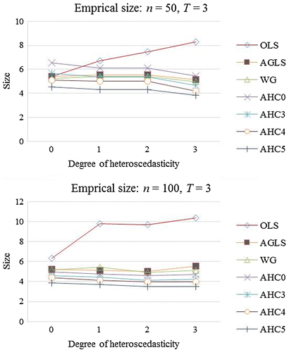
Empirical sizes are displayed in Figure 1 at 5% LOS and ${\sigma }_v^2=2$. The OLSE curve shows high over-rejection. While the curves produced by the AGLSE and WGE are closer to nominal LOS (5%). The curve of AHC0 shows deviation from nominal level (5%) under mild and moderate heteroscedasticity but becomes closer to 5% under severe heteroscedasticity for small sample. However, the AHC0 gets improvement in performance for large sample. Similar results have been reported by Long and Ervin (2000) for cross-sectional data. The AHC4 and AHC5 curves are closer to the nominal LOS (5%).

Figure 1. Empirical size (%) for β.

Tables 3 and 4 display empirical sizes for Schemes I and II, respectively. In Table 3, the test based on the OLS variance estimator is largely liberal under smaller UTVH (${\sigma }_v^2=2$). It expresses high size distortion for the cases of heteroscedasticity. Under severe heteroscedasticity ($\lambda$ = 3), the NRR produced by the OLS variance estimator based quasi-t test is 8.30% at 5% LOS for smaller UTVH (${\sigma }_v^2=2$). However, the quasi-t test, based on the OLS variance estimator, gives better NRR for the larger UTVH (${\sigma }_v^2=6$). The quasi-t test, based on the AGLS variance estimator, performs better than the test based on the OLS variance estimator. For instance, for $\lambda =3$, the NRR yields by AGLS variance estimator based quasi-t test is 5.14% at 5% LOS for smaller UTVH (${\sigma }_v^2=2$). It verifies the reported results of Roy. The quasi-t tests that employ AHCCMEs yield good NRR from smaller UTVH (${\sigma }_v^2=2$) to the larger UTVH (${\sigma }_v^2=6$). The best NRR among the AHCCMEs, is observed by the tests based on AHC4 and AHC5. In case of severe heteroscedasticity ($\lambda =3$), the AHC4 yields exact NRR for ${\sigma }_v^2=6$ at 5% LOS. The results given by the AHC4 and AHC5 confirm the findings made by Cribari-Neto (Cribari-Neto, 2004) and Cribari-Neto et al. (Cribari-Neto et al., 2007) for the non-panel data and also justify their formulation for the PDM.

Table 3. NRR of quasi-t test for N = 50, T = 3

${\sigma }_v^2$	2			4			6
α	1%	5%	10%	1%	5%	10%	1%	5%	10%
	λ = 0
OLS	1.04	5.40	11.48	1.26	5.40	10.28	0.86	5.08	10.26
AGLS	1.20	5.42	10.46	1.42	5.44	10.76	1.34	5.58	10.60
WG	1.32	5.24	10.34	1.26	5.22	10.06	1.24	5.48	10.96
AHC0	1.78	6.52	11.30	1.90	6.04	12.16	1.66	6.48	11.66
AHC3	1.38	5.66	10.28	1.62	5.24	10.68	1.38	5.68	10.60
AHC4	1.26	5.10	9.62	1.46	4.92	9.88	1.22	5.24	9.96
AHC5	0.92	4.54	8.52	1.30	4.28	8.60	1.02	4.62	9.20
λ = 1
OLS	1.50	6.70	12.60	1.86	7.02	12.86	1.44	5.58	11.42
AGLS	1.00	5.52	10.58	1.46	5.78	10.80	1.20	5.76	10.78
WG	1.12	5.42	10.58	1.24	5.42	10.56	1.10	5.44	10.30
AHC0	1.36	6.12	11.26	1.88	6.52	11.80	1.48	6.42	11.88
AHC3	1.04	5.38	10.08	1.64	5.58	10.60	1.26	5.28	10.50
AHC4	0.92	5.00	9.46	1.40	5.26	9.86	1.08	4.82	9.80
AHC5	0.80	4.32	8.30	1.20	4.74	8.80	0.86	4.24	8.74
λ = 2
OLS	1.76	7.46	13.62	1.88	7.32	12.88	1.76	6.20	11.94
AGLS	1.34	5.52	10.06	1.34	5.50	11.12	1.42	5.92	11.24
WG	1.24	5.42	10.08	0.96	5.30	10.90	1.16	5.68	10.78
AHC0	1.66	6.12	11.28	1.58	6.46	11.94	1.64	6.96	12.30
AHC3	1.30	5.38	10.26	1.34	5.82	10.48	1.28	6.14	11.08
AHC4	1.12	5.00	9.60	1.22	5.08	9.96	1.18	5.66	10.50
AHC5	0.96	4.32	8.68	1.06	4.48	9.04	1.04	5.12	9.68
λ = 3
OLS	1.94	8.30	14.56	1.74	7.14	12.58	1.62	6.50	11.82
AGLS	0.98	5.14	10.36	1.02	5.12	10.86	1.48	5.96	11.52
WG	0.94	4.98	9.82	0.84	5.06	9.98	1.36	5.88	10.46
AHC0	1.26	5.46	11.18	1.30	6.26	11.58	1.62	6.48	12.10
AHC3	1.00	4.64	10.10	1.04	5.50	10.34	1.22	5.76	10.80
AHC4	0.88	4.16	9.32	0.96	4.98	9.62	1.06	5.00	10.24
AHC5	0.80	3.84	8.30	0.88	4.14	8.52	0.92	4.42	9.36

Table 4. NRR of quasi-t test for N = 100, T = 3

${\sigma }_v^2$	2			4			6
α	1%	5%	10%	1%	5%	10%	1%	5%	10%
	λ = 0
OLS	1.78	6.34	11.88	1.50	6.88	12.36	1.06	5.94	11.30
AGLS	1.22	5.22	10.24	1.56	6.46	11.60	1.30	5.74	10.88
WG	1.08	5.20	10.38	1.36	5.76	11.68	1.26	5.50	10.74
AHC0	1.16	4.94	9.90	1.74	6.22	11.46	1.30	5.50	10.36
AHC3	1.02	4.60	9.26	1.64	5.86	11.04	1.16	5.06	9.82
AHC4	0.84	4.38	8.76	1.42	5.44	10.60	1.08	4.82	9.42
AHC5	0.76	3.88	7.96	1.16	4.80	9.52	0.78	4.44	8.74
λ = 1
OLS	2.52	9.80	16.66	2.34	8.46	14.98	1.70	7.00	13.26
AGLS	1.04	5.10	10.62	1.36	5.68	10.98	1.16	5.96	11.42
WG	0.94	5.42	10.26	1.16	5.42	10.26	0.98	4.62	10.06
AHC0	1.02	4.78	9.70	1.18	5.42	10.60	1.14	5.86	11.20
AHC3	0.86	4.44	8.80	1.04	4.98	9.86	1.02	5.52	10.48
AHC4	0.84	4.14	8.40	1.02	4.72	9.58	0.98	5.18	9.98
AHC5	0.70	3.72	7.64	0.86	4.10	8.90	0.80	4.54	9.14
λ = 2
OLS	2.80	9.66	16.62	2.26	8.22	14.28	1.58	6.40	12.20
AGLS	1.02	5.00	10.28	1.24	5.60	10.34	1.30	5.18	10.64
WG	1.14	4.92	9.42	1.08	5.34	10.02	1.08	5.36	10.04
AHC0	1.02	4.58	9.46	1.30	5.28	9.86	1.22	5.02	10.58
AHC3	0.96	4.14	8.80	1.14	4.68	9.24	1.08	4.64	9.60
AHC4	0.90	3.96	8.42	1.06	4.56	8.96	0.98	4.44	9.34
AHC5	0.72	3.52	7.54	0.98	4.04	8.28	0.90	4.16	8.50
λ = 3
OLS	3.38	10.36	17.04	2.88	8.64	15.12	1.72	7.08	12.74
AGLS	1.02	5.52	10.40	1.26	5.00	9.72	1.24	5.30	10.92
WG	0.88	5.10	10.16	1.12	4.68	9.48	0.96	4.98	10.16
AHC0	0.90	4.68	9.92	1.12	4.76	8.90	1.18	5.30	10.60
AHC3	0.78	4.22	9.16	1.06	4.32	8.24	1.02	4.68	10.06
AHC4	0.70	3.96	8.70	1.02	4.12	7.84	1.00	4.44	9.70
AHC5	0.64	3.50	7.80	0.90	3.74	7.30	0.90	3.94	8.98

In Table 4, behavior of all the estimators is similar as presented in Table 3. The tests, based on the AGLSE variance estimator, perform well in terms of NRR as reported by Roy (Roy, 2002). Performance of the AHC4 and AHC5 remains attractive and justifies our proposal for the PDM.

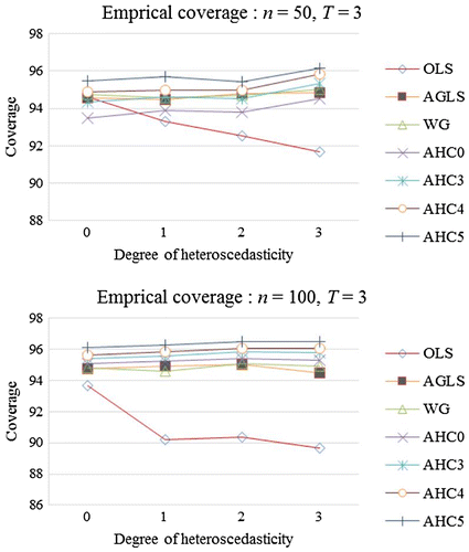
Estimation of confidence interval is done as illustrated in Equation (13). For ${\sigma }_v^2=2$, empirical coverage is presented in Figure 2. The OLSE curve exhibits under-coverage, while the curve of AGLSE is closer to the nominal coverage (95%). The curve of AHC0 shows under-coverage for small sample but coverage rate is closer to the nominal coverage (95%) for the large samples. On the other side, the curves of AHC4 and AHC5 are closer to the nominal coverage (95%).

Figure 2. Empirical coverage (%) for β.

For the above-mentioned estimators, Tables 5 and 6 carry empirical coverage and average length for Schemes I and II, respectively. Performance of the OLSE is not satisfactory in for smaller UTVH as it shows under-coverage. However, the OLSE gets improvement in performance from smaller (${\sigma }_v^2=2$) to larger UTVH (${\sigma }_v^2=6$). While the AGLSE shows remarkable performance for homoscedastic as well as for all types of heteroscedastic cases. The empirical coverage of the WGE is closer to nominal coverage (95%) for all degrees of heteroscedasticity and it outperforms the OLSE. It is noticed that the best empirical coverage among AHCCMEs are produced by our AHC4 and AHC5. The AHC4 exhibits exact coverage for ${\sigma }_v^2=2$ in case of mild heteroscedasticity ($\lambda =1$) and also for larger UTVH (${\sigma }_v^2=6$) when $\lambda =3$. The AHC5-based confidence intervals display coverage that is close to the nominal coverage (95%).

Table 5. 95% Confidence interval: coverage (%) and length (N = 50, T = 3)

${\sigma }_{\upsilon }^2$	2		4		6
	Coverage	Length	Coverage	Length	Coverage	Length
	λ = 0
OLS	94.60	1.69	94.60	1.69	94.92	1.70
AGLS	94.58	1.02	94.56	1.38	94.42	1.61
WG	94.76	1.09	94.78	1.47	94.52	1.96
AHC0	93.48	1.00	93.96	1.36	93.52	1.59
AHC3	94.34	1.04	94.76	1.42	94.32	1.65
AHC4	94.90	1.07	95.08	1.46	94.76	1.69
AHC5	95.46	1.12	95.72	1.53	95.38	1.76
λ = 1
OLS	93.30	1.70	92.98	1.70	94.42	1.70
AGLS	94.48	1.02	94.22	1.39	94.24	1.61
WG	94.58	1.10	94.58	1.48	94.56	1.96
AHC0	93.88	1.01	93.48	1.38	93.58	1.59
AHC3	94.62	1.05	94.42	1.43	94.72	1.65
AHC4	95.00	1.08	94.74	1.47	95.18	1.70
AHC5	95.68	1.12	95.26	1.54	95.76	1.76
λ = 2
OLS	92.54	1.70	92.68	1.70	93.80	1.70
AGLS	94.80	1.02	94.50	1.39	94.08	1.62
WG	94.72	1.10	94.70	1.48	94.32	1.96
AHC0	93.82	1.01	93.54	1.38	93.04	1.60
AHC3	94.52	1.05	94.18	1.44	93.86	1.66
AHC4	94.98	1.08	94.92	1.48	94.34	1.70
AHC5	95.44	1.12	95.52	1.54	94.88	1.77
λ = 3
OLS	91.70	1.70	92.86	1.71	93.50	1.71
AGLS	94.86	1.02	94.88	1.39	94.04	1.62
WG	95.02	1.10	94.94	1.48	94.12	1.96
AHC0	94.54	1.01	93.74	1.38	93.52	1.61
AHC3	95.36	1.05	94.50	1.44	94.24	1.68
AHC4	95.84	1.08	95.02	1.47	95.00	1.72
AHC5	96.16	1.13	95.86	1.54	95.58	1.78

Table 6. 95% Confidence interval: coverage (%) and length (N = 100, T = 3)

${\sigma }_v^2$	2		4		6
	Coverage	Length	Coverage	Length	Coverage	Length
	λ = 0
OLS	93.66	1.24	93.12	1.24	94.06	1.24
AGLS	94.78	0.77	93.54	1.04	94.26	1.19
WG	94.80	0.83	94.24	1.12	94.50	1.37
AHC0	95.06	0.79	93.78	1.06	94.50	1.20
AHC3	95.40	0.80	94.14	1.08	94.94	1.23
AHC4	95.62	0.82	94.56	1.09	95.18	1.24
AHC5	96.12	0.84	95.20	1.13	95.56	1.28
λ =1
OLS	90.20	1.25	91.54	1.25	93.00	1.25
AGLS	94.90	0.77	94.32	1.05	94.04	1.05
WG	94.58	0.83	94.58	1.12	95.38	1.12
AHC0	95.22	0.80	94.58	1.07	94.14	1.07
AHC3	95.56	0.81	95.02	1.09	94.48	1.09
AHC4	95.86	0.83	95.28	1.11	94.82	1.11
AHC5	96.28	0.86	95.90	1.14	95.46	1.14
λ = 2
OLS	90.34	1.25	91.78	1.25	93.60	1.25
AGLS	95.00	0.77	94.40	1.05	94.82	1.05
WG	95.08	0.84	94.66	1.12	94.64	1.12
AHC0	95.42	0.80	94.72	1.07	94.98	1.07
AHC3	95.86	0.98	95.32	1.10	95.36	1.10
AHC4	96.04	0.83	95.44	1.11	95.56	1.11
AHC5	96.48	0.85	95.96	1.15	95.84	1.15
λ = 3
OLS	89.64	1.25	91.36	1.25	92.92	1.25
AGLS	94.48	0.77	95.00	1.05	94.70	1.05
WG	94.90	0.84	95.32	1.12	95.02	1.12
AHC0	95.32	0.80	95.24	1.08	94.70	1.08
AHC3	95.78	0.82	95.68	1.10	95.32	1.10
AHC4	96.04	0.83	95.88	1.11	95.56	1.11
AHC5	96.50	0.85	96.26	1.15	96.06	1.15

Performance of the estimators in Table 6 is similar to that observed in Table 5. For the large samples, Roy’s estimator outperforms the OLSE. Among the AHCCME, AHC4 and AHC5 express very good coverage and average interval length and they remain attractive choice.

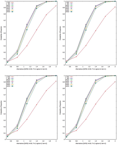
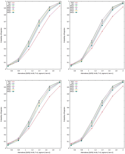
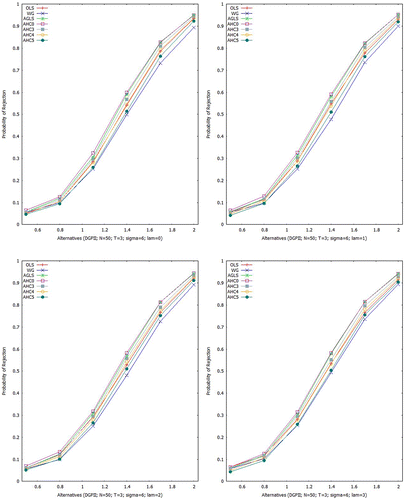
Figures 3^{Figure 4}–5 show empirical power curves, built upon all the above mentioned estimators for Scheme I. For ${\sigma }_v^2=2$, Figure 3 gives indication that for homoscedastic ($\lambda =0$) and heteroscedastic situations ($\lambda =1$, 2 and 3), all the estimators show identical power of test to that of the AGLSE except OLSE. However, as ${\sigma }_v^2$ increases, the OLSE gets improvement in such a way that for ${\sigma }_v^2=6$, all the estimators become near to identical in power of test. Table 7 gives numerical values of the empirical power for a specific case i.e. ${\sigma }_v^2=2,N=50,T=3.$ Aslam (2006) presented power curve analysis of the above mentioned estimators in context of the PDM and our results verify his findings.

Figure 3. Empirical power at 5% LOS (N = 50, T = 3; ${\sigma }_v^2=2$).

Figure 4. Empirical power at 5% LOS (N = 50, T = 3; ${\sigma }_v^2=4$).

Figure 5. Empirical power at 5% LOS (N = 50, T = 3; ${\sigma }_v^2=6$).

Table 7. Power results (%) for ${\sigma }_v^2=2,N=50,T=3$

OLS	AGLS	AHC0	AHC3	AHC4	AHC5
		λ = 0
5.40	5.42	6.52	5.66	5.10	4.54
12.14	21.76	22.92	20.86	19.46	17.34
30.16	63.66	63.72	61.16	58.98	55.26
55.20	92.88	93.06	91.76	90.74	88.72
78.78	99.60	99.56	99.38	99.26	98.86
92.76	99.99	99.99	99.99	99.98	99.98
λ = 1
6.70	5.42	5.52	6.12	5.38	4.32
13.00	20.20	20.88	22.10	20.02	17.28
30.54	60.98	63.02	63.64	60.34	54.84
53.84	91.98	92.80	92.80	91.68	88.42
76.44	99.28	99.60	99.50	99.34	98.64
90.98	99.99	99.98	99.98	99.98	99.92
λ = 2
7.46	5.28	5.20	6.18	5.48	4.56
13.96	20.80	21.64	22.74	20.48	17.52
31.44	62.42	64.00	64.50	61.72	56.00
54.52	91.98	93.24	93.22	91.76	88.48
76.48	99.32	99.52	99.56	99.46	99.00
91.36	99.99	99.99	99.99	99.98	99.92
λ = 3
8.30	4.98	5.14	5.46	4.16	3.84
14.12	20.62	21.84	23.32	20.26	18.52
31.60	61.70	63.60	63.96	59.12	56.12
55.50	92.04	93.20	93.16	90.56	88.42
75.70	99.52	99.60	99.44	99.22	98.72
90.30	99.99	99.99	99.99	99.99	99.96

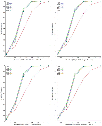
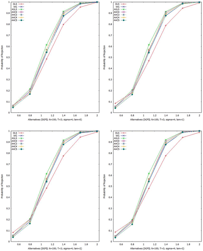
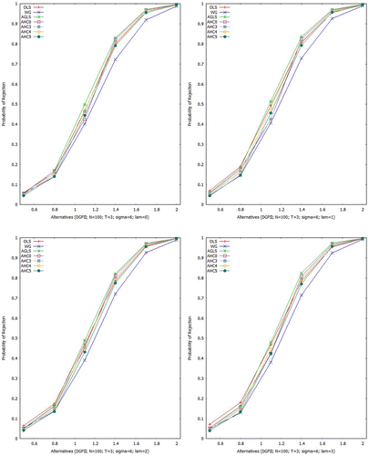
For all the estimators under consideration, empirical power curves for Scheme II are displayed in Figures 6^{Figure 7}–8. In case of larger sample, it is noticed that power curves of all the estimators get slumber. Performance of the OLSE is not good for smaller UTVH (${\sigma }_v^2=2$) but it becomes closer to the AGLSE for larger UTVH (${\sigma }_v^2=6$).

Figure 6. Empirical power at 5% LOS (N = 100, T = 3; ${\sigma }_v^2=2$).

Figure 7. Empirical power at 5% LOS (N = 100, T = 3; ${\sigma }_v^2=4$).

Figure 8. Empirical power at 5% LOS (N = 100, T = 3; ${\sigma }_v^2=6$).

6. Illustrative example

We take an example of panel data of productivity of USA (Munnell, 1990) with T = 17 and N = 48. The model of interest is(14) $$y_{\mathit{it}}={\beta }_0+{\beta }_1{x}_{1it}+{\beta }_2{x}_{2it}+{\beta }_3{x}_{3it}+{\beta }_4{x}_{4it}+{\beta }_5{x}_{5it}+{\beta }_6{x}_{6it}+u_{\mathit{it}};(i=1,2,\dots ,48,t=1,2,\dots ,17),$$(14)

where y denotes gross production, x₁ is high way capital, x₂ is water utility capital, x₃ is utility capital, x₄ is private capital, x₅ is employed capital, and x₆ is unemployed capital.

In order to evaluate the testing performance of all the stated estimators, following Cribari-Neto (2004), an extra variable (e.g. $x_5^2$) is being added as an explanatory variable. Thus, Model (14) is reformulated as(15) $$y_{\mathit{it}}={\beta }_0+{\beta }_1{x}_{1it}+{\beta }_2{x}_{2it}+{\beta }_3{x}_{3it}+{\beta }_4{x}_{4it}+{\beta }_5{x}_{5it}+{\beta }_6{x}_{6it}+{\beta }_7{x}_{5it}^2+u_{\mathit{it}}.$$(15)

The USH is found after the Wald test (with p-value < 0.01). Table 8 displays the comparative statistics obtained from Model (14). The results obtained from fitting of Model (15) are presented in Table 8. All the regression coefficients are found to be statistically significant while referring to Table 7. In Model (15), we include square of employed capital as an extra explanatory variable with the expectedly no impact on determining the gross production. Thus, it should be statistically non-significant. We perform the inference again. In this situation, the attractive estimator would be one that does not reject the null hypothesis of β₇ = 0. Table 9 shows that the tests based on only AHC4 and AHC5 do not reject the hypothesis of β₇ = 0 at 1% LOS.

Table 8. Comparative statistic of model (14)

	OLS	AGLS	WG	AHC0	AHC3	AHC4	AHC5
${\widehat{\beta }}_0$	1.926	2.148	2.192	–	–	–	–
${\widehat{\beta }}_1$	0.058	0.064	0.077	–	–	–	–
${\widehat{\beta }}_2$	0.199	0.077	0.079	–	–	–	–
${\widehat{\beta }}_3$	0.009	–0.096	–0.115	–	–	–	–
${\widehat{\beta }}_4$	0.312	0.273	0.235	–	–	–	–
${\widehat{\beta }}_5$	0.550	0.746	0.801	–	–	–	–
${\widehat{\beta }}_6$	−0.007	−0.006	−0.005	–	–	–	–
$se({\widehat{\beta }}_0)$	0.053	0.138	0.216	1.005	1.024	1.034	1.038
$se({\widehat{\beta }}_1)$	0.015	0.022	0.031	0.113	0.115	0.116	0.116
$se({\widehat{\beta }}_2)$	0.012	0.014	0.015	0.038	0.039	0.039	0.039
$se({\widehat{\beta }}_3)$	0.012	0.017	0.018	0.054	0.055	0.056	0.056
$se({\widehat{\beta }}_4)$	0.011	0.020	0.026	0.146	0.151	0.155	0.157
$se({\widehat{\beta }}_5)$	0.016	0.025	0.030	0.162	0.167	0.172	0.174
$se({\widehat{\beta }}_6)$	0.014	0.001	0.001	0.003	0.003	0.004	0.004
$t({\widehat{\beta }}_0)$	36.684	15.576	10.132	2.138	2.099	2.076	2.070
$t({\widehat{\beta }}_1)$	3.821	2.968	2.457	0.565	0.556	0.552	0.552
$t({\widehat{\beta }}_2)$	9.597	5.556	5.245	2.001	1.981	1.969	1.967
$t({\widehat{\beta }}_3)$	0.692	−5.712	−6.325	−1.771	−1.739	−1.725	−1.723
$t({\widehat{\beta }}_4)$	28.142	13.786	8.964	1.857	1.805	1.756	1.739
$t({\widehat{\beta }}_5)$	35.380	29.948	26.924	4.597	4.460	4.346	4.291
$t({\widehat{\beta }}_6)$	−5.255	−6.766	−5.288	−1.753	−1.709	−1.674	−1.659
$p({\widehat{\beta }}_0)$	0.000	0.000	0.000	0.000	0.000	0.000	0.000
$p({\widehat{\beta }}_1)$	0.000	0.000	0.000	0.007	0.008	0.008	0.008
$p({\widehat{\beta }}_2)$	0.000	0.000	0.000	0.000	0.000	0.000	0.000
$p({\widehat{\beta }}_3)$	0.003	0.000	0.000	0.000	0.000	0.000	0.000
$p({\widehat{\beta }}_4)$	0.000	0.000	0.000	0.000	0.000	0.000	0.000
$p({\widehat{\beta }}_5)$	0.000	0.000	0.000	0.000	0.000	0.000	0.000
$p({\widehat{\beta }}_6)$	0.000	0.000	0.000	0.000	0.000	0.000	0.000

Table 9. Comparative statistic of model (15)

	OLS	AGLS	WG	AHC0	AHC3	AHC4	AHC5
${\widehat{\beta }}_0$	3.368	2.604	2.489	–	–	–	–
${\widehat{\beta }}_1$	0.003	0.052	0.071	–	–	–	–
${\widehat{\beta }}_2$	0.128	0.076	0.079	–	–	–	–
${\widehat{\beta }}_3$	0.010	−0.089	−0.112	–	–	–	–
${\widehat{\beta }}_4$	0.323	0.270	0.228	–	–	–	–
${\widehat{\beta }}_5$	0.190	0.631	0.736	–	–	–	–
${\widehat{\beta }}_6$	−0.007	−0.006	−0.005	–	–	–	–
${\widehat{\beta }}_7$	0.027	0.009	0.006	–	–	–	–
$se({\widehat{\beta }}_0)$	0.146	0.260	0.329	1.465	1.497	1.518	1.531
$se({\widehat{\beta }}_1)$	0.015	0.021	0.032	0.111	0.113	0.114	0.114
$se({\widehat{\beta }}_2)$	0.012	0.014	0.015	0.037	0.037	0.037	0.037
$se({\widehat{\beta }}_3)$	0.012	0.017	0.018	0.054	0.055	0.053	0.055
$se({\widehat{\beta }}_4)$	0.010	0.019	0.027	0.137	0.142	0.146	0.152
$se({\widehat{\beta }}_5)$	0.037	0.057	0.064	0.231	0.242	0.253	0.276
$se({\widehat{\beta }}_6)$	0.001	0.001	0.001	0.003	0.003	0.003	0.004
$se({\widehat{\beta }}_7)$	0.003	0.004	0.005	0.016	0.016	0.017	0.017
$t({\widehat{\beta }}_0)$	23.132	9.997	7.572	1.778	1.739	1.715	1.700
$t({\widehat{\beta }}_1)$	0.193	2.392	2.236	0.467	0.459	0.456	0.455
$t({\widehat{\beta }}_2)$	10.982	5.564	5.268	2.087	2.058	2.048	2.042
$t({\widehat{\beta }}_3)$	0.823	−5.377	−6.141	−1.665	−1.634	−1.624	−1.620
$t({\widehat{\beta }}_4)$	30.955	13.966	8.504	1.975	1.909	1.854	1.776
$t({\widehat{\beta }}_5)$	5.130	11.022	11.492	2.732	2.609	2.499	2.284
$t({\widehat{\beta }}_6)$	−5.492	−6.716	−5.119	−1.778	−1.727	−1.689	−1.645
$t({\widehat{\beta }}_7)$	10.524	2.115	1.198	0.552	0.535	0.522	0.501
$p({\widehat{\beta }}_0)$	0.000	0.000	0.000	0.000	0.000	0.000	0.000
$p({\widehat{\beta }}_1)$	0.104	0.000	0.000	0.015	0.015	0.015	0.016
$p({\widehat{\beta }}_2)$	0.000	0.000	0.000	0.000	0.000	0.000	0.000
$p({\widehat{\beta }}_3)$	0.001	0.000	0.000	0.000	0.000	0.000	0.000
$p({\widehat{\beta }}_4)$	0.000	0.000	0.000	0.000	0.000	0.000	0.000
$p({\widehat{\beta }}_5)$	0.000	0.000	0.000	0.000	0.000	0.000	0.000
$p({\widehat{\beta }}_6)$	0.000	0.000	0.000	0.000	0.000	0.000	0.000
$p({\widehat{\beta }}_7)$	0.000	0.000	0.000	0.008	0.009	0.011	0.012

7. Conclusion

To improve the testing of coefficients of the PDM with the problem of USH, we have used the HCCMEs, based on Roy’s (2002) adaptive estimator. It is found that the AHC4 and AHC5 perform better than all the competing estimators in terms of NRR, power of tests and empirical coverage of interval estimators. On the basis of our findings, the adaptive versions of HCCME are found to be as attractive choice for the testing of PDM as they are for the linear regression models with heteroscedastic errors.

Funding

The authors received no direct funding for this research.

Additional information

Notes on contributors

Afshan Saeed

Muhammad Aslam is a tenured associate professor at the Department of Statistics, Bahauddin Zakariya University, Multan, Pakistan. He acquires a teaching experience of more than 20 years at postgraduate level. His main area of interest runs around the inference of linear regression models with issues of heteroscedasticity and multicollinearity. He has conducted a number of researches in the stated area while leading a research team, comprising of his research students and few colleagues. Recently, this team has developed three R packages, namely “mctest”, “lmridge”, and “liureg” which are available on the R CRAN. These are comprehensive packages for detection of multicollinearity, estimation of the ridge and Liu regression models with different choices of penalties. The present article is a part of PhD research project of Afshan Saeed (the Principal author) under the supervision of Aslam. This article, primarily addresses the inference of panel data model with the issue of unit-specific heteroscedasticity.

References

- Ahmed, M., Aslam, M., & Pasha, G. R. (2011). Inference under heteroscedasticity of unknown form using an adaptive estimator. Communications in Statistics – Theory and Methods, 40, 4431–4457.10.1080/03610926.2010.513793
- Arellano, M. (1987). Computing robust standard errors for within-group estimators. Oxford Bulletin of Economics and Statistics, 49, 431–434.
- Aslam, M. (2006). Adaptive procedures for estimation of linear regression models with known and unknown heteroscedastic errors ( dissertation). Pakistan: Bahauddin Zakariya University.
- Aslam, M., Riaz, T., & Altaf, S. (2013). Efficient estimation and robust inference of linear regression models in the presence of heteroscedastic errors and high leverage points. Communications in Statistics – Simulation and Computation, 42, 2223–2238.10.1080/03610918.2012.695847
- Baltagi, B. H., & Griffin, M. (1988). A generalized error component model with heteroscedastic disturbances. International Economic Review, 29, 745–753.10.2307/2526831
- Baltagi, B. H., Bresson, G., & Pirotte, A. (2004). Adaptive estimation of heteroskedastic error component models. USA: Texas A & M University, Working Paper.
- Cribari-Neto, F. (2004). Asymptotic inference under heteroskedasticity of unknown form. Computational Statistics & Data Analysis, 45, 215–233.10.1016/S0167-9473(02)00366-3
- Cribari-Neto, F., & Lima, M. G. A. (2009). Heteroskedasticity-consistent interval estimators. Journal of Statistical Computation and Simulation, 79, 787–803.10.1080/00949650801935327
- Cribari-Neto, F., Souza, T. C., & Vasconcellos, K. L. P. (2007). Inference under heteroskedasticity and leveraged data. Communications in Statistics – Theory and Methods, 36, 1877–1888.10.1080/03610920601126589
- Eicker, F. (1963). Asymptotic normality and consistency of the least squares estimators for families of linear regressions. The Annals of Mathematical Statistics, 34, 447–456.10.1214/aoms/1177704156
- Greene, W. H. (1997). Econometric analysis (3rd ed.). Upper Saddle River, NJ: Prentice Hall.
- Hoaglin, D. C., & Welsch, R. E. (1978). The hat matrix in regression and ANOVA. American Statistical, 32, 17–22.
- Li, Q., & Stengos, T. (1994). Adaptive estimation in the panel data error component model with heteroscedasticity of unknown form. International Economic Review, 35, 981–1000.10.2307/2527006
- Long, J. S., & Ervin, L. H. (2000). Using heteroscedasticity consistent standard errors in the linear regression model. American Statistical, 54, 217–224.
- Mazodier, P., & Trognon, A. (1978). Heteroscedasticity and stratification in error components models. Anna. de l’Insee, 30–31, 451–482.
- Munnell, A. H. (1990). Why has productivity growth declined? Productivity and public investment. New England: Economic Review.
- Randolph, W. C. (1988). A transformation for heteroksedastic error components regression models. Economics Letters, 27, 349–354.10.1016/0165-1765(88)90161-9
- Rilstone, P. (1991). Some Monte Carlo evidence on the relative efficiency of parametric and semi parametric EGLS estimators. Journal of Business & Economic Statistics, 9, 179–187.
- Roy, N. (2002). Is adaptive estimation useful for panel models with heteroscedasticity in the individual specific error component? Some monte carlo evidence Economic Review, 21, 189–203.
- Uchôa, C. F. A., Cribari-Neto, F., & Menezes, T. A. (2014). Testing inference in heteroscedastic fixed effects models. European Journal of Operational Research, 235, 660–670.10.1016/j.ejor.2014.01.032
- White, H. (1980). A heteroscedasticity-consistent covariance matrix estimator and a direct test for heteroscedasticity. Econometrica, 48, 817–838.10.2307/1912934