Stochastic outlook of two non-identical unit parallel system with priority in repair

Abstract

The crux of the study is to investigate a two non-identical unit parallel system where priority is given to first unit. The system consists of two non-identical units arranged in parallel configuration. System failure occurs when both the units stop Working. Weibull failure and repair time distributions of each unit are taken. Several measures of system effectiveness, such as reliability, MTSF, steady state availability, expected profit etc., useful to system managers are obtained by using regenerative point technique. Further, recognizing the fact that the life testing experiments are very time consuming, the parameters representing the reliability characteristics of the system/unit are assumed to be random variables. Both informative and non-informative prior are used for the Bayesian analysis. Therefore, a simulation study is also conducted for analysing the considered system model both in classical and Bayesian setups.

Keywords:

• MTSF
• profit function
• Weibull
• availability
• repair

AMS classification 2010:

• 90B25
• 65F35
• 62F10
• 62F15

Public Interest Statement

The determination of the reliability measures of a complex system, composed of a number of interconnected subsystems, has received much attention over the years. The most of the above studies were mainly concerned to obtain various reliability characteristics such as meantime to system failure (MTSF), point wise and steady state availabilities etc., by using exponential distribution as failure and repair time distribution of units but not to estimate the parameter(s) involved in the life time/repair time distribution of system/unit. Similarly, in real world, assuming constant failure and repair time distribution of units is not realistic. Therefore, the present study aims to investigate a two non-identical unit parallel system where priority is given to first unit with non-Markovian behaviors of hazard and repair along with estimation problem of unknown parameters.

1. Introduction

Any equipment or system manufactured is designed with assured objectives to meet up its goals in terms of production/service. A reliable equipment is the one which works satisfactorily for a given time period under given environmental conditions without any interruptions. A high degree of reliability is an absolute necessity. No one can afford to take risk with a device which does not operate particularly at an instant when human life and national security is at stake.

Besides this, the complexity of technological system and their products are increasing day by day and hence thrown a challenge before designers, engineers, manufactures for the reliable performance of their system. Therefore, the objectives of reliability are many fold and include the following (Mishra, 2006):

•	adequate performance of system/equipment for a specified duration
•	hang on to precise environmental conditions
•	control on downtime of system/equipment
•	crisis free running of system/equipment

Reliability measures are very effective and efficient tool for probabilistic risk assessment in system design, operation and maintenance. The determination of the reliability measures of a complex system composed of a number of interconnected subsystems has received much attention over the years. Gupta and Sharma (1993), Rehmert and Nachlas (2009), Ghasemi, Yacout, and Ouali (2010) have reported substantial work in the field of reliability analysis, by considering complex systems with different failure and repair policy.

Reliability analysis of parallel systems has been broadly studied by Gupta and Agarwal(1984), Dhillon and Anuda (1993a, 1993b), Sridharan and Mohanavadivu (1997), Kumar, Bharti, and Gupta (2012) and the reference cited therein. Dhillon and Anuda (1993a) studied the common cause failure analysis of a two non-identical unit parallel system with arbitrarily distributed repair times. Chopra and Ram (2017) study stochastic analysis of two non-identical unit parallel system incorporating waiting time. El-Sherbeny (2017) investigates the influence of the system parameters on a system consisting of a 2-unit cold standby system with a single repair person. Considering the issue of high cost of similar units and giving priority to one of the units in repair as compared to other, Malik, Bhardwaj, and Grewal (2010) develop a reliability model for a system of non-identical units-one is original and the other unit as duplicate (called sub-standard unit). However, there may be a situation, where priority to a specified unit in repair may be given to avoid unnecessary inspections e.g. In the hilly region, there are two roads named A and B, respectively. Both are non-identical units i.e. road A is a highway whereas road B is a link road. Both roads connect to the same destination from same starting place and work parallel. In tight corner, such as snowfall, landslide etc. while both roads A and B get damaged, priority of repairing is given to road A in lieu of road B. Second instance, there are two non-identical turbines “X” and “Y” are working parallel. Turbine X has more capacity than turbine Y. In those circumstances, when both turbines stopped working, turbine X gets priority in repairing.

The most of the of the above studies were mainly concerned to obtain various reliability characteristics such as meantime to system failure (MTSF), point wise and steady state availabilities etc., by using exponential distribution as failure and repair time distribution of units and not to estimate the parameter(s) involved in the life time/repair time distribution of system/unit. However, in real world, assuming constant failure and repair time distribution of units is not realistic. The Weibull distribution has been widely used in reliability and survival analysis, especially for describing the fatigue failures. Weibull (1951) used this distribution for vacuum tube failures while Lieblein and Zelen (1956) consider it for ball bearing failures. Singh, Rathi, and Kumar (2013) attempt classical and Bayesian analysis of a k-components load-sharing parallel system model assuming the failure time distribution of the components as Weibull. Chaturvedi, Pati, and Tomer (2014) consider robust Bayesian analysis of the Weibull failure model under a sigma-contamination class of priors for the parameters. Recently, Gupta and Singh (2017) performed classical and Bayesian analysis of Weibull parameters in presence of outlier. Also, Dey, Alzaatreh, Zhang, and Kumar (2017) introduce a new generalization of Weibull distribution called alpha-power transformed Weibull distribution that provides better fits than the Weibull distribution and some of its known generalizations. We refer to Mann (1968) and the reference cited therein, where Weibull distribution gives a variety of situations in which this distribution can be used for various types of data.

In view of the above concerns, the purpose of the present study is to two fold. First, we analyse a two non-identical unit parallel system model by incorporating Weibull distribution for both failure and repair times with same shape parameter but different scale parameters. It is well known that the Weibull distribution has been frequently used in life-testing and survival analysis especially for describing the fatigue failures. Weibull (1951) utilized this model for vacuum tube failures and Lieblein and Zelen (1956) also assumed the same for ball bearing failures. Singh et al. (2013) analysed the k-components load-sharing parallel system model by considering the failure time distribution of the load-sharing components as Weibull. Recently, Gupta and Singh (2017) considered the parameter estimation of Weibull model in presence of outlier. We refer to Mann (1968) and the reference cited therein, where Weibull distribution gives a variety of situations in which this distribution can be used for various types of data.

Secondly, on the other hand, assuming the parameters involved in the model as random variable, a simulation study is attempted for analysing the considered model in classical as well as Bayesian set-up. ML estimates of the parameters, MTSF and Profit function with their standard errors (SEs) and corresponding length of the confidence interval are observed. For obtaining Bayes estimates, we assumed both informative and non-informative prior for the model parameters. At the end, comparison is made through simulation study to judge the performance of ML and Bayes estimates for various values of the failure and repair parameters.

2. System model description, notations and states of the system

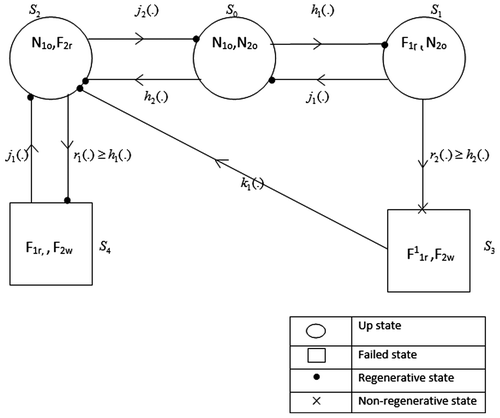
The system made by two non-identical units (unit-1 and unit-2) arranged in parallel network. Each unit has two Modes-Normal (N) and total failure (F). The first unit has priority in repair. Units will be work as good as new after repair. System will fail when both units stop working. The failure rate of operative unit has increased when system operates with only one unit in comparison to the situation when both the units are operative. The failure and repair time distribution of each unit are taken to be independent having the Weibull density with common shape parameter λ and different scale parameters α and β as follows:$$f_i(t)={\alpha }_i\lambda t^{\lambda -1}exp(-{\alpha }_i{t}^{\lambda }),$$

and$$g_i(t)={\beta }_i\lambda t^{\lambda -1}exp(-{\beta }_i{t}^{\lambda }),$$

where t ≥ 0; α_i and β_i, λ > 0 and i = 1, 2, respectively, for unit-1 and unit-2.

2.1. Notations

Table

E	Set of regenerative states = {S0, S1, S2, S4}
αi/βi	Scale parameter of failure/repair time distribution of ith unit
λ	Shape parameter of failure/repair time distribution of each unit
hi(t)	Failure rate of ith unit when both the units are operational in the parallel network; $h_i(t)={\alpha }_{i}p{t}^{\lambda -1},{\alpha }_i,\lambda ,t>0$
ri(t)	Increased failure rate of ith unit$r_i(t)={\mu }_{i}p{t}^{\lambda -1},{\mu }_i,\lambda ,t>0$
ji(t)	Repair rate of ith unit; $j_i(t)={\beta }_{i}p{t}^{\lambda -1},{\beta }_i,\lambda ,t>0$
qij(.)	Probability density function of one step or direct transition time from Si ∊ E to Sj ∊ E
Qij(.)	Cumulative distribution function of one step or direct transition time from Si ∊ E to Sj ∊ E
pij	Steady state transition probability from state Si ∊ E to Sj ∊ E such that $p_{\mathit{ij}}=\underset{t\to \infty }{lim}{Q}_{\mathit{ij}}(t)$
$p_{\mathit{ij}}^{(k)}$	Steady state transition probability from state Si ∊ E to Sj ∊ E via state Sk ∊ E such that $p_{\mathit{ij}}^{(k)}=\underset{t\to \infty }{lim}{Q}_{\mathit{ij}}^{(k)}(t)$
ψi	Mean sojourn time in state Si i.e. ${\psi }_i={\int }_0^{\infty }P[T_i>t]dt$
Ri(t)	Reliability of the system at time t when system starts from state Si
Ai(t)	Probability that the system will be operative busy in state Si ∊ E at epoch t
Bi(t)	Probability that the repairman will be busy in state Si ∊ E at epoch t
τup(t)	Expected up time of the system during interval (0, t) i.e.${\tau }_{\mathit{up}}(t)=\underset{0}{\overset{t}{\int }}{A}_0(u)du$
τb(t)	Expected busy period of repairman during interval (0, t) i.e.${\tau }_b(t)=\underset{0}{\overset{t}{\int }}{B}_0(u)du$
pf(t)	Profit incurred by the system during interval (0, t)
*	Symbol of Laplace transformation of a function i.e. $q_{\mathit{ij}}^{\ast }={\int }_0^{\infty }{e}^{-st}{q}_{\mathit{ij}}(t)dt$
•	Regenerative point
×	Non-regenerative point
@	Used for convolution i.e. ${\int }_0^{t}M(u)U(t-u)du=M(t)@U(t)$

2.2. Symbols for the states of the system

Table

N1o	Unit-1 is in N-mode and operative
N2o	Unit-2 is in N-mode and operative
F1r	Unit-1 is in F-mode and under repair
F2r	Unit-2 is in F-mode and under repair
F2w	Unit-2 is in F-mode and under waiting for repair
$F_{1r}^1$	First unit is in failure mode and its repair is continued from state S1

Using the above symbols, the possible states of the system are represented in the transition diagram shown in Figure 1 where S₀, S₁ and S₂ are the up states and S₃ and S₄ are failed states. It is also verified that the state S₃is non-regenerative state.

Figure 1. Transition diagram.

3. Transition probabilities, sojourn times and conditional mean sojourn times

3.1. Transition probabilities

Transition probability matrix (TPM) of the implanted Markov Chain is given by:$$P=\left(\begin{array}{cccc}{p}_{00}& p_{01}& p_{02}& p_{04}\\ p_{10}& p_{11}& p_{12}^{(3)}& p_{14}\\ p_{20}& p_{21}& p_{22}& p_{24}\\ p_{40}& p_{41}& p_{42}& p_{44}\end{array}\right)$$

With non-zero elements:(1) $$\left.\begin{array}{c}{p}_{01}=\frac{{\alpha }_1}{({\alpha }_1+{\alpha }_2)},p_{02}=\frac{{\alpha }_2}{({\alpha }_1+{\alpha }_2)},p_{10}=\frac{{\beta }_1}{({\beta }_1+{\mu }_2)},\hfill \\ p_{12}^{(3)}=\frac{{\mu }_2}{({\beta }_1+{\mu }_2)},p_{20}=\frac{{\beta }_2}{({\beta }_2+{\mu }_1)},p_{24}=\frac{{\mu }_1}{({\beta }_2+{\mu }_1)},p_{42}=1\hfill \end{array}\right\}$$(1)

and the other elements of TMP will be zero.

Without loss of generality, the following expressions can be easily obtained p₀₁ + p₀₂ = 1, $p_{10}+p_{12}^{(3)}=1$, p₂₀ + p₂₄ = 1.

3.2. Sojourn times

The corresponding value of the mean sojourn time ψ_i; i = 0, 1, 2, 4 for various regenerative states are as follows:(2) $$\left.\begin{array}{c}{\psi }_0=\frac{\mathrm{\Gamma }(1/\lambda )}{\lambda {({\alpha }_1+{\alpha }_2)}^{1/\lambda }},{\psi }_1=\frac{\mathrm{\Gamma }(1/\lambda )}{\lambda {({\beta }_1+{\mu }_2)}^{1/\lambda }}\hfill \\ {\psi }_2=\frac{\mathrm{\Gamma }(1/\lambda )}{\lambda {({\mu }_1+{\beta }_2)}^{1/\lambda }},{\psi }_4=\frac{\mathrm{\Gamma }(1/\lambda )}{\lambda {\beta }^{1/\lambda }}\hfill \end{array}\right\}$$(2)

Conditional mean sojourn time:

Values of the conditional mean sojourn time for various regenerative states are as follows:(3) $$\left.\begin{array}{c}{m}_{01}=\mathrm{\Gamma }\left(1+\frac{1}{\lambda }\right)\frac{{\alpha }_1}{{({\alpha }_1+{\alpha }_2)}^2},m_{02}=\mathrm{\Gamma }\left(1+\frac{1}{\lambda }\right)\frac{{\alpha }_2}{{({\alpha }_1+{\alpha }_2)}^2}\hfill \\ m_{10}=\mathrm{\Gamma }\left(1+\frac{1}{\lambda }\right)\frac{{\beta }_1}{{({\beta }_1+{\mu }_2)}^2},m_{12}^{(3)}=\mathrm{\Gamma }\left(1+\frac{1}{\lambda }\right)\frac{{\mu }_2}{{({\beta }_1+{\mu }_2)}^2}\hfill \\ m_{20}=\mathrm{\Gamma }\left(1+\frac{1}{\lambda }\right)\frac{{\beta }_2}{{({\mu }_1+{\beta }_2)}^2},m_{24}=\mathrm{\Gamma }\left(1+\frac{1}{\lambda }\right)\frac{{\mu }_1}{{({\mu }_1+{\beta }_2)}^2}\hfill \\ m_{42}=\mathrm{\Gamma }\left(1+\frac{1}{\lambda }\right)\frac{1}{\beta 1}\hfill \end{array}\right\}$$(3)

4. Measures of system effectiveness

4.1. Reliability and MTSF of the system

To determine R_i(t), we consider the failed state S₃ and S₄ of the system as absorbing state. By the probabilistic arguments, we have:(4) $$R_0(t)=Z_0(t)+q_{01}@R_1(t)+q_{02}@R_2(t)$$(4) (5) $$R_1(t)=Z_1(t)+q_{10}@R_0(t)$$(5) (6) $$R_2(t)=Z_2(t)+q_{20}@R_0(t)$$(6)

where $Z_0(t)=e^{-({\alpha }_1+{\alpha }_2)t^{\lambda }}$, $Z_1(t)=e^{-({\beta }_1+{\mu }_2)t^{\lambda }}$ and $Z_2(t)=e^{-({\mu }_1+{\beta }_2)t^{\lambda }}$.

Taking Laplace transformations of Equations (4), (5) and (6) and simplifying for $R_0^{\ast }(s)$, we get:(7) $$R_0^{\ast }(s)=\frac{Z_0^{\ast }+q_{01}^{\ast }{Z}_1^{\ast }+q_{02}^{\ast }{Z}_2^{\ast }}{(1-q_{01}^{\ast }{q}_{10}^{\ast }-q_{02}^{\ast }{q}_{20}^{\ast })}$$(7)

After obtaining the inverse Laplace transformations of equation (7), one can easily get the reliability of the system when it initially starts from stateS₀.

When system primarily starts from state S₀, the MTSF is given by:(8) $$E(T_0)=\underset{0}{\overset{\infty }{\int }}{R}_0(t)dt=\underset{s\to 0}{lim}{R}_0^{\ast }(s)=\frac{{\psi }_0+p_{01}{\psi }_1+p_{02}{\psi }_2}{(1-p_{01}{p}_{10}-p_{02}{p}_{20})}$$(8)

4.2. Availability analysis

By simple probabilistic arguments, we have the following recursive relation in A_i(t):(9) $$A_0(t)=Z_0(t)+q_{01}(t)@A_1(t)+q_{02}(t)@A_2(t)$$(9) (10) $$A_1(t)=Z_1(t)+q_{10}(t)@A_0(t)+q_{12}^{(3)}(t)@A_2(t)$$(10) (11) $$A_2(t)=Z_2(t)+q_{20}(t)@A_0(t)+q_{24}(t)@A_4(t)$$(11) (12) $$A_4(t)=q_{42}(t)@A_2(t)$$(12)

After taking the Laplace transform of equations (9), (10), (11) and (12) and simplifying for $A_0^{\ast }(s)$, we get(13) $$A_0^{\ast }(t)=\frac{N_1(s)}{D_1(s)}=\frac{(1-q_{24}^{\ast }{q}_{42}^{\ast })(Z_0^{\ast }+q_{01}^{\ast }{Z}_1^{\ast })+Z_2^{\ast }(q_{01}^{\ast }{q}_{12}^{{(3)}^{\ast }}+q_{02}^{\ast })}{(1-q_{24}^{\ast }{q}_{42}^{\ast })(1-q_{01}^{\ast }{q}_{10}^{\ast })-q_{20}^{\ast }(q_{01}^{\ast }{q}_{12}^{{(3)}^{\ast }}+q_{02}^{\ast })}$$(13)

Taking inverse Laplace transform of equation (13), we can get availability of the system for known value of parameters.

In the long run, the steady state probability that the system will be operate, is given by:(14) $$A_0=\underset{t\to \infty }{lim}{A}_0(t)=\underset{s\to 0}{lim}S{A}_0^{\ast }(s)=\frac{p_{20}({\psi }_0+p_{01}{\psi }_1)+{\psi }_2(1-p_{01}{p}_{10})}{p_{20}(1+m_{01}+m_{02})+(1-p_{01}{p}_{10})(1+m_{20}+m_{24}+p_{24}{m}_{42})+p_{01}{p}_{20}(m_{10}+m_{12}^{(3)})}$$(14)

The expected up time of the system during time interval (0, t) is given by:$${\tau }_{\mathit{up}}(t)={\int }_0^t{A}_0(u)du$$

So that:(15) $${\tau }_{\mathit{up}}^{\ast }(s)=\frac{A_0^{\ast }(s)}{S}$$(15)

4.3. Busy period analysis

By simple probabilistic arguments, we have the following recursive relation in B_i(t): (i = 0, 1, 2, 4):(16) $$B_0(t)=q_{01}(t)@B_1(t)+q_{02}(t)@B_2(t)$$(16) (17) $$B_1(t)=Z_4(t)+q_{12}^{(3)}(t)@B_2(t)+q_{10}(t)@B_0(t)$$(17) (18) $$B_2(t)=Z_2(t)+q_{24}(t)@B_4(t)+q_{20}(t)@B_0(t)$$(18) (19) $$B_4(t)=Z_4(t)+q_{42}(t)@B_2(t)$$(19)

where, $Z_4(t)=e^{-{\beta }_1{t}^{\lambda }}$.

Taking the Laplace transformation of relations (16, 17, 18 and 19) and simplifying for $B_0^{\ast }(s)$, omitting the argument’s’ for brevity, we get:(20) $$B_0^{\ast }(t)=\frac{N_2(s)}{D_1(s)}=\frac{(Z_2^{\ast }+q_{24}^{\ast }{Z}_4^{\ast })(q_{01}^{\ast }{q}_{12}^{{(3)}^{\ast }}+q_{02}^{\ast })+q_{01}^{\ast }{Z}_4^{\ast }(1-q_{24}^{\ast }{q}_{42}^{\ast })}{(1-q_{24}^{\ast }{q}_{42}^{\ast })(1-q_{01}^{\ast }{q}_{10}^{\ast })-q_{20}^{\ast }(q_{01}^{\ast }{q}_{12}^{\ast }+q_{02}^{\ast })}$$(20)

In the long run, the steady state probability that the repairman will be busy in the repair of a failed unit, is, given by:(21) $$B_0=\underset{t\to \infty }{lim}{B}_0(t)=\underset{s\to 0}{lim}S{B}_0^{\ast }(s)=\frac{({\psi }_2+p_{24}{\psi }_4)(p_{01}{p}_{12}^{(3)}+p_{02})+p_{01}{p}_{20}{\psi }_4}{p_{20}(1+m_{01}+m_{02})+(1-p_{01}{p}_{10})(1+m_{20}+m_{24}+p_{24}{m}_{42})+p_{01}{p}_{20}(m_{10}+m_{12}^{(3)})}$$(21)

The expected busy period of the repairman during time interval (0, t) is:$${\tau }_b(t)={\int }_0^t{B}_0(u)du$$

So that(22) $${\tau }_b^{\ast }(s)=\frac{B_0^{\ast }(s)}{S}$$(22)

4.4. Profit analysis

The net expected profit incurred by the system during the time interval (0, t) is given by:(23) $$pt\left(t\right)=K_0{\tau }_{\mathit{up}}\left(t\right)-K_1{\tau }_b\left(t\right)$$(23)

where K₀ is the revenue per unit up time by the system and K₁is the amount paid to the repairman per unit time when the system is under repair. The net expected profit incurred by the system per unit of time in steady state is given by:(24) $$P=K_0{A}_0-K_1{B}_0$$(24)

where A₀ and B₀ has been defined already in previous sections.

5. Estimation of parameters, MTSF and profit function

5.1. Classical estimation

Let us assume that the failure, increased failure and repair times are independently Weibull-distributed random variables with failure rates h₁(.),h₂(.) increased failure ratesr₁(.), r₂(.) and the repair ratesj₁(.), j₂(.), respectively, where:

$h_i(t)={\alpha }_{i}p{t}^{\lambda -1}$, $r_i(t)={\mu }_{i}p{t}^{\lambda -1}$ and $g_i(t)={\beta }_{i}p{t}^{\lambda -1}$t > 0, ${\alpha }_i,{\beta }_i,{\mu }_i,\lambda >0(i=1,2)$

Here α_i, β_i μ_i and are scale parameters while λ is the shape parameter.

In our study, we are interested with the ML estimation procedure as one of the most important classical procedures.$${\underset{\sim }{Z}}_i=(x_{i1},x_{i2}\dots ,x_{i{n}_i});i=1,2,\dots ,6$$

Let six independent samples of size $n_j(j=1,\dots ,6)$ drown from Weibull distribution with failure rates h₁(.), h₂(.), r₁(.), r₂(.) and repair rates j₁(.), j₂(.), respectively

The likelihood function of the combined sample is:(25) $$L\left({\underset{\sim }{Z}}_1,{\underset{\sim }{Z}}_2,{\underset{\sim }{Z}}_3,{\underset{\sim }{Z}}_4,{\underset{\sim }{Z}}_5,{\underset{\sim }{Z}}_6|{\alpha }_1,{\alpha }_2,{\mu }_1,{\mu }_2,{\beta }_1,{\beta }_2\right)={\alpha }_1^{n_1}{\alpha }_2^{n_2}{\mu }_1^{n_3}{\mu }_2^{n_4}{\beta }_1^{n_5}{\beta }_2^{n_6}{\lambda }^{(n_1+n_2+n_3+n_4+n_5+n_6)}\times \prod _{i=1}^6\prod _{j=1}^{n_1}{z}_{\mathit{ij}}^{\lambda -1}{e}^{\left({\alpha }_1\sum _{j=1}^{n_1}{z}_{1j}^{\lambda }+{\alpha }_2\sum _{j=1}^{n_2}{z}_{2j}^{\lambda }+{\mu }_1\sum _{j=1}^{n_3}{z}_{3j}^{\lambda }+{\mu }_2\sum _{j=1}^{n_4}{z}_{4j}^{\lambda }+{\beta }_1\sum _{j=1}^{n_5}{z}_{5j}^{\lambda }+{\beta }_2\sum _{j=1}^{n_6}{z}_{6j}^{\lambda }\right)}$$(25)

By using maximization likelihood approach, the ML estimates (say ${\widehat{\alpha }}_1,{\widehat{\alpha }}_2,{\widehat{\mu }}_1,{\widehat{\mu }}_2,{\widehat{\beta }}_1,{\widehat{\beta }}_2$) of the parameters α₁, α₂, μ₁, μ₂, β₁, β₂$${\widehat{\alpha }}_1=\frac{n_1}{\sum _{j=1}^{n_1}{z}_{1j}^{\lambda }};{\widehat{\alpha }}_2=\frac{n_2}{\sum _{j=1}^{n_2}{z}_{2j}^{\lambda }};{\widehat{\mu }}_1=\frac{n_3}{\sum _{j=1}^{n_3}{z}_{3j}^{\lambda }}$$$${\widehat{\mu }}_2=\frac{n_4}{\sum _{j=1}^{n_4}{z}_{4j}^{\lambda }};{\widehat{\beta }}_1=\frac{n_5}{\sum _{j=1}^{n_5}{z}_{5j}^{\lambda }};{\widehat{\beta }}_2=\frac{n_6}{\sum _{j=1}^{n_6}{z}_{6j}^{\lambda }}$$

Without loss of generality, using the invariance property of MLE, the MLEs of MTSF and profit function, say $\widehat{M}$ and $\widehat{P}$ can be easily obtained. The asymptotic distribution of ${\left({\widehat{\alpha }}_1-{\alpha }_1,{\widehat{\alpha }}_2-{\alpha }_2,{\widehat{\mu }}_1-{\mu }_1,{\widehat{\mu }}_2-{\mu }_2,{\widehat{\beta }}_1-{\beta }_1,{\widehat{\beta }}_2-{\beta }_2\right)}^{{}^{\prime }}\sim N_6(0,I^{-1})$

where I denotes the Fisher information matrix with diagonal elements$$I_{11}=\frac{n_1}{{\alpha }_1^2};I_{22}=\frac{n_2}{{\alpha }_2^2};I_{33}=\frac{n_3}{{\mu }_1^2};I_{44}=\frac{n_4}{{\mu }_2^2};I_{55}=\frac{n_5}{{\beta }_1^2};I_{66}=\frac{n_6}{{\beta }_2^2}$$

Also non diagonal elements are all zero.

Also, the asymptotic distribution of $(\widehat{M}-M)\sim N_6(0,A^{{}^{\prime }}{I}^{-1}A)$ and $(\widehat{P}-P)\sim N_6(0,B^{{}^{\prime }}{I}^{-1}B)$

where

$A^{{}^{\prime }}=\left(\frac{\partial M}{\partial {\alpha }_1},\frac{\partial M}{\partial {\alpha }_2},\frac{\partial M}{\partial {\mu }_1},\frac{\partial M}{\partial {\mu }_2},\frac{\partial M}{\partial {\beta }_1},\frac{\partial M}{\partial {\beta }_2}\right)$ and $B^{{}^{\prime }}=\left(\frac{\partial P}{\partial {\alpha }_1},\frac{\partial P}{\partial {\alpha }_2},\frac{\partial P}{\partial {\mu }_1},\frac{\partial P}{\partial {\mu }_2},\frac{\partial P}{\partial {\beta }_1},\frac{\partial P}{\partial {\beta }_2}\right)$

5.2. Bayesian estimation

Assuming the parameters involved in the model as random variable, we have also considered the Bayesian methods of estimation. The prior distributions of scale parameters α₁, α₂, μ₁, μ₂, β₁, β₂(when the shape parameter λ is known) are assumed to be gamma distribution with parameters (θ_i, δ_i; i = 1, 2, …, 6) and are given as follows:(26) $$\begin{array}{c}{\alpha }_1\sim Gamma({\theta }_1,{\delta }_1)\hfill \\ {\alpha }_2\sim Gamma({\theta }_2,{\delta }_2)\hfill \\ {\mu }_1\sim Gamma({\theta }_3,{\delta }_3)\hfill \\ {\mu }_2\sim Gamma({\theta }_4,{\delta }_4)\hfill \\ {\beta }_1\sim Gamma({\theta }_5,{\delta }_5)\hfill \\ {\beta }_2\sim Gamma({\theta }_6,{\delta }_6)\hfill \end{array}$$(26)

Here, the parameters of prior distributions are called hyper parameters. Using the likelihood function in equation (25) and prior distribution of α₁, α₂, μ₁, μ₂, β₁, β₂ considered in the Equation (26), the posterior distributions are as follows:(27) $${\alpha }_1|{\underset{\sim }{Z}}_1\sim Gamma(n_1+{\theta }_1,{\delta }_1+\sum _{j=1}^{n_1}{z}_{1j}^{\lambda })$$(27) (28) $${\alpha }_2|{\underset{\sim }{Z}}_2\sim Gamma(n_2+{\theta }_2,{\delta }_2+\sum _{j=1}^{n_2}{z}_{2j}^{\lambda })$$(28) (29) $${\mu }_1|{\underset{\sim }{Z}}_3\sim Gamma(n_3+{\theta }_3,{\delta }_3+\sum _{j=1}^{n_3}{z}_{3j}^{\lambda })$$(29) (30) $${\mu }_2|{\underset{\sim }{Z}}_4\sim Gamma(n_4+{\theta }_4,{\delta }_4+\sum _{j=1}^{n_4}{z}_{4j}^{\lambda })$$(30) (31) $${\beta }_1|{\underset{\sim }{Z}}_5\sim Gamma(n_5+{\theta }_5,{\delta }_5+\sum _{j=1}^{n5}{z}_{5j}^{\lambda })$$(31) (32) $${\beta }_2|{\underset{\sim }{Z}}_6\sim Gamma(n_6+{\theta }_6,{\delta }_6+\sum _{j=1}^{n_6}{z}_{6j}^{\lambda })$$(32)

Under the squared error loss function, Bayes estimates of α₁, α₂, μ₁, μ₂, β₁, β₂ are, respectively, the means of posterior distribution given in Equations (27)–(32) and as follows:(33) $$\begin{array}{c}{\widehat{\alpha }}_1=\frac{{\delta }_1+\sum _{j=1}^{n_1}{z}_{1j}^{\lambda }}{n_1+{\theta }_1};{\widehat{\alpha }}_2=\frac{{\delta }_2+\sum _{j=1}^{n_2}{z}_{2j}^{\lambda }}{n_2+{\theta }_2};{\widehat{\mu }}_1=\frac{{\delta }_3+\sum _{j=1}^{n_3}{z}_{3j}^{\lambda }}{n_3+{\theta }_3}\hfill \\ {\widehat{\mu }}_2=\frac{{\delta }_4+\sum _{j=1}^{n_4}{z}_{4j}^{\lambda }}{n_4+{\theta }_4};{\widehat{\beta }}_1=\frac{{\delta }_5+\sum _{j=1}^{n5}{z}_{5j}^{\lambda }}{n_5+{\theta }_5};{\widehat{\beta }}_2=\frac{{\delta }_6+\sum _{j=1}^{n_6}{z}_{6j}^{\lambda }}{n_6+{\theta }_6}\hfill \end{array}$$(33)

6. Simulation study

In this section, a simulation study is performed to validate the theoretical developments. The standard errors of the estimates and widths of the confidence/HPD intervals are used for comparison purpose. Since, the shape of the hazard rate of Weibull lifetime model is increasing, decreasing and constant as well for different values of the shape parameter; hence, we assume the following values of the model parameters to conduct the simulation study:

•	n = 100, β1 = 0.6, β2 = 0.5, μ1 = 0.5, μ2 = 0.6 Z and λ = 0.75
•	n = 100, β1 = 0.7, β2 = 0.5, μ1 = 0.5, μ2 = 0.6 and λ = 0.75
•	n = 100, β1 = 0.6, β2 = 0.5, μ1 = 0.5, μ2 = 0.6 and λ = 1.00
•	n = 100, β1 = 0.7, β2 = 0.5, μ1 = 0.5, μ2 = 0.6 and λ = 1.00
•	n = 100, β1 = 0.6, β2 = 0.5, μ1 = 0.5, μ2 = 0.6 and λ = 1.25
•	n = 100, β1 = 0.7, β2 = 0.5, μ1 = 0.5, μ2 = 0.6 and λ = 1.25

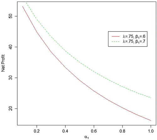
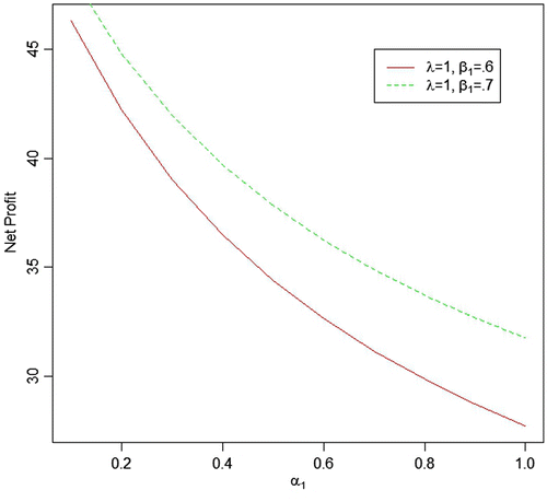
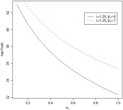
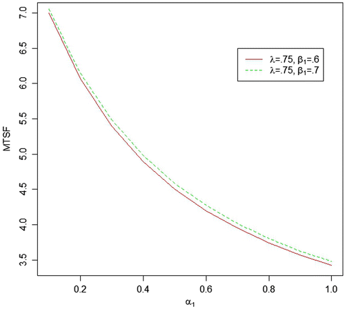
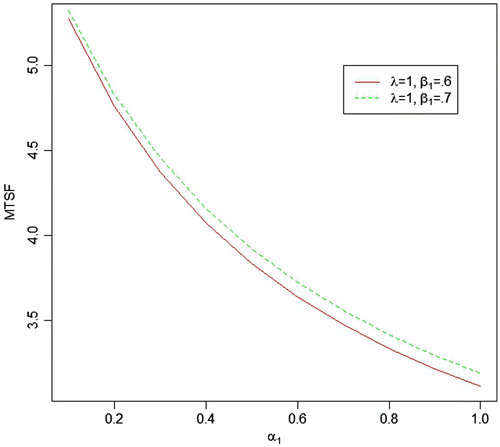
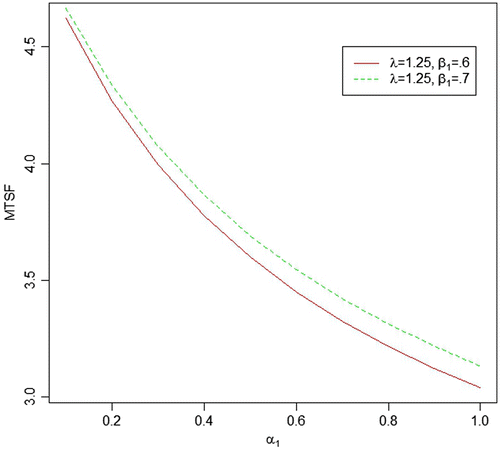
We generated six data sets with respect to the above-mentioned different values of parameters, respectively, and based on these data sets, the MLEs and Bayes estimates (for both informative and non-informative prior) for the parameters, system MTSF and net profit have been obtained. Bayes estimates of the parameters with gamma priors have been obtained by setting the values of prior’s parameters as α₁ = E(α₁) = δ₁/θ₁and similarly for rest of the model parameters and put the values of all prior’s parameters as zero to obtain Bayes estimates with Jeffrey’s priors. The various estimates of the MTSF and Profit along with their SEs/PSEs and length of the confidence/HPD intervals have been summarized in Table 1–12. The value of the constant K₀ and K₁ are taken as 150 and 50, respectively. For more real study of the system, we have also plot curves of the MTSF and net profit for different values of α₁, β₁ and λ while keeping the other parameters fix. For all the numerical computations, the programs are developed in R-environment and are available with the authors.

Table 1. Various estimates of MTSF for fixed λ = 0.75, β₁ = 0.6 and varying α₁

α1	0.1	0.2	0.3	0.4	0.5	0.6	0.7	0.8	0.9	1
True value	7.0012	6.0658	5.395	4.8933	4.5056	4.1981	3.9489	3.7434	3.5714	3.4255
ML estimate	6.8121	5.5924	5.0294	4.8966	4.3758	4.7377	3.619	3.4317	3.808	3.2959
SE	0.5832	0.4558	0.3876	0.3135	0.2908	0.2481	0.2715	0.2565	0.2164	0.2243
Width	2.2861	1.7866	1.5195	1.229	1.1399	0.9725	1.0643	1.0055	0.8482	0.8793
Bayes (prior 1)	6.8749	5.6341	5.0711	4.9314	4.4033	4.7675	3.6434	3.4568	3.8341	3.3205
PSE (prior 1)	0.5676	0.4018	0.3538	0.3192	0.2779	0.3071	0.2295	0.2231	0.2489	0.211
Width (prior 1)	2.2165	1.5716	1.3818	1.2467	1.084	1.1968	0.8967	0.8691	0.9711	0.817
Bayes (prior 2)	6.4333	5.2741	4.7502	4.6203	4.1432	4.4812	3.451	3.2967	3.6566	3.1772
PSE (prior 2)	0.511	0.3608	0.3215	0.2876	0.2556	0.2795	0.2101	0.2059	0.2283	0.1912
Width (prior 2)	1.9866	1.4115	1.2593	1.1146	0.9963	1.0867	0.8191	0.7981	0.8905	0.7479

Table 2. Various estimates of profit for fixed λ = 0.75, β₁ = 0.6 and varying α₁

α1	0.1	0.2	0.3	0.4	0.5	0.6	0.7	0.8	0.9	1
True value	53.184	44.8483	38.4234	33.3082	29.1341	25.6612	22.7257	20.2118	18.0349	16.1318
ML estimate	52.7559	42.3372	36.3184	31.8297	28.6704	36.4906	21.1317	22.6804	15.2387	17.3026
SE	0.5832	0.4558	0.3876	0.3135	0.2908	0.2481	0.2715	0.2565	0.2164	0.2243
Width	2.2861	1.7866	1.5195	1.229	1.1399	0.9725	1.0643	1.0055	0.8482	0.8793
Bayes (prior 1)	52.8146	42.2806	36.2207	31.6117	28.3943	36.2737	20.8894	22.4037	14.7947	17.0764
PSE (prior 1)	4.4096	4.0954	4.1398	4.8329	4.7632	4.3083	4.5675	4.6886	6.0513	4.6433
Width (prior 1)	17.3298	16.0988	16.2963	18.8687	18.534	16.7767	17.8149	18.2358	23.4473	18.161
Bayes (prior 2)	51.2001	41.1753	35.4611	31.4057	28.5575	35.9103	21.4325	23.2511	16.9169	18.3683
PSE (prior 2)	4.1243	3.7459	3.8497	4.4247	4.3298	3.9348	4.2245	4.2702	5.3435	4.1618
Width (prior 2)	16.0197	14.714	15.1162	17.463	16.821	15.4447	16.5926	16.6122	20.7971	16.1877
PSE (prior 2)	0.3081	0.2687	0.2174	0.2115	0.1986	0.1886	0.1804	0.1746	0.1667	0.1519
Width (prior 2)	1.1959	1.0497	0.8483	0.8295	0.7777	0.7356	0.7045	0.6797	0.6481	0.5914

Table 3. Various estimates of MTSF for fixed λ = 1.00, β₁ = 0.6 and varying α₁

α1	0.1	0.2	0.3	0.4	0.5	0.6	0.7	0.8	0.9	1
True value	5.2778	4.7619	4.375	4.0741	3.8333	3.6364	3.4722	3.3333	3.2143	3.1111
ML estimate	4.9404	4.7736	4.1895	4.1216	3.9103	3.709	3.4554	3.3707	3.1988	2.9076
SE	0.3714	0.2835	0.2565	0.2241	0.2069	0.1936	0.1937	0.1891	0.1798	0.1872
Width	1.4559	1.1113	1.0056	0.8785	0.811	0.759	0.7591	0.7414	0.7047	0.7337
Bayes (prior 1)	4.9741	4.7991	4.2096	4.1426	3.9305	3.7272	3.4718	3.3873	3.215	2.9238
PSE (prior 1)	0.3331	0.2931	0.2351	0.2295	0.2173	0.2014	0.1935	0.1871	0.1795	0.1619
Width (prior 1)	1.3027	1.1432	0.9179	0.8929	0.8475	0.7937	0.7562	0.729	0.6986	0.6308
Bayes (prior 2)	4.7343	4.5668	4.0093	3.9485	3.751	3.5661	3.3358	3.2601	3.1057	2.8391
PSE (prior 2)	0.3081	0.2687	0.2174	0.2115	0.1986	0.1886	0.1804	0.1746	0.1667	0.1519
Width (prior 2)	1.1959	1.0497	0.8483	0.8295	0.7777	0.7356	0.7045	0.6797	0.6481	0.5914

Table 4. Various estimates of profit for fixed λ = 1.00, β₁ = 0.6 and varying α₁

α1	0.1	0.2	0.3	0.4	0.5	0.6	0.7	0.8	0.9	1
True value	46.3344	42.2192	39.0365	36.4873	34.3915	32.6332	31.1338	29.838	28.7058	27.707
ML estimate	44.722	41.4767	37.9684	36.9418	36.047	31.8167	32.8345	33.8714	26.3754	26.1278
SE	0.3714	0.2835	0.2565	0.2241	0.2069	0.1936	0.1937	0.1891	0.1798	0.1872
Width	1.4559	1.1113	1.0056	0.8785	0.811	0.759	0.7591	0.7414	0.7047	0.7337
Bayes (prior 1)	44.7376	41.4306	37.9147	36.8774	35.9654	31.7388	32.7281	33.8117	26.2743	26.0453
PSE (prior 1)	3.0515	3.1108	3.1406	3.2016	3.2539	3.2772	3.3306	3.0419	3.2318	3.2449
Width (prior 1)	11.9527	12.1882	12.2633	12.5817	12.7111	12.8116	12.9382	11.8709	12.6295	12.6862
Bayes (prior 2)	43.9176	40.8249	37.4399	36.5649	35.7073	31.7855	32.8606	33.7545	26.7923	26.6369
PSE (prior 2)	2.9249	2.9379	2.9678	3.0315	3.0254	3.1209	3.0989	2.8593	3.034	3.059
Width (prior 2)	11.4407	11.5851	11.638	11.8667	11.7925	12.2873	12.107	11.1863	11.8989	11.9829

Table 5. Various estimates of MTSF for fixed λ = 1.25, β₁ = 0.6 and varying α₁

α1	0.1	0.2	0.3	0.4	0.5	0.6	0.7	0.8	0.9	1
True value	4.6237	4.2684	3.9948	3.777	3.5991	3.4509	3.3252	3.2173	3.1234	3.041
ML estimate	4.2282	4.2213	4.0005	3.8559	3.7088	3.2678	3.4438	3.4523	3.205	2.8021
SE	0.3037	0.2238	0.2165	0.191	0.1776	0.1809	0.1665	0.1514	0.1634	0.1692
Width	1.1906	0.8772	0.8489	0.7487	0.6962	0.7091	0.6527	0.5937	0.6407	0.6633
Bayes (prior 1)	4.2514	4.2391	4.0174	3.8696	3.7229	3.2826	3.458	3.4676	3.2196	2.814
PSE (prior 1)	0.2642	0.2235	0.2092	0.1959	0.1895	0.1609	0.1753	0.1804	0.1636	0.1449
Width (prior 1)	1.0275	0.8721	0.8145	0.762	0.7394	0.6302	0.6814	0.7037	0.6377	0.5658
Bayes (prior 2)	4.0939	4.0742	3.8597	3.7208	3.5851	3.1706	3.3383	3.3578	3.1264	2.756
PSE (prior 2)	0.2457	0.209	0.1943	0.1826	0.1769	0.1512	0.1645	0.1684	0.1546	0.137
Width (prior 2)	0.9646	0.8126	0.7538	0.7129	0.6914	0.5897	0.6408	0.6598	0.6028	0.5324

Table 6. Various estimates of profit for fixed λ = 1.25, β₁ = 0.6 and varying α₁

α1	0.1	0.2	0.3	0.4	0.5	0.6	0.7	0.8	0.9	1
True value	42.9649	40.5963	38.7895	37.3507	36.1681	35.172	34.3169	33.5717	32.9139	32.3274
ML estimate	40.1195	38.9066	41.5474	40.0765	38.2753	33.1655	36.6432	34.2651	34.3813	30.112
SE	0.3037	0.2238	0.2165	0.191	0.1776	0.1809	0.1665	0.1514	0.1634	0.1692
Width	1.1906	0.8772	0.8489	0.7487	0.6962	0.7091	0.6527	0.5937	0.6407	0.6633
Bayes (prior 1)	40.0894	38.8552	41.5009	39.9954	38.216	33.1379	36.5854	34.2139	34.3413	30.0679
PSE (prior 1)	2.5856	2.7232	2.7087	2.8056	2.6839	2.8337	2.6991	2.8937	2.81	2.8867
Width (prior 1)	10.1242	10.7033	10.6036	10.9661	10.5538	11.0557	10.5146	11.2569	10.9159	11.3507
Bayes (prior 2)	39.7758	38.6437	41.1335	39.7622	38.0188	33.162	36.4834	34.4076	34.4337	30.4828
PSE (prior 2)	2.4619	2.622	2.5831	2.6737	2.5703	2.7046	2.5909	2.7376	2.6829	2.7544
Width (prior 2)	9.7112	10.2256	10.016	10.4878	10.0412	10.5196	10.149	10.6622	10.494	10.7177

Table 7. Various estimates of MTSF for fixed λ = 0.75, β₁ = 0.7 and varying α₁

α1	0.1	0.2	0.3	0.4	0.5	0.6	0.7	0.8	0.9	1
True value	7.0602	6.1468	5.4823	4.9796	4.5875	4.2743	4.019	3.8073	3.6293	3.4778
ML estimate	7.0753	6.6917	5.4378	5.6135	4.2505	4.5564	4.0321	4.1689	3.7923	3.7198
SE	0.5712	0.4196	0.384	0.308	0.3092	0.2653	0.257	0.2267	0.2243	0.2126
Width	2.2392	1.645	1.5053	1.2072	1.2119	1.0401	1.0073	0.8888	0.8794	0.8333
Bayes (prior 1)	7.1369	6.7389	5.4804	5.6527	4.2786	4.5842	4.0606	4.1979	3.8173	3.7459
PSE (prior 1)	0.5758	0.4822	0.3866	0.3797	0.2755	0.295	0.2636	0.2671	0.2429	0.2388
Width (prior 1)	2.2327	1.8734	1.5037	1.4714	1.066	1.1486	1.0302	1.0438	0.9437	0.9334
Bayes (prior 2)	6.6718	6.2781	5.1218	5.2789	4.0232	4.3133	3.8387	3.9707	3.6342	3.5757
PSE (prior 2)	0.515	0.4319	0.3453	0.3398	0.2503	0.2684	0.2411	0.2442	0.2226	0.2183
Width (prior 2)	2.009	1.6844	1.3346	1.3205	0.978	1.0456	0.9512	0.9502	0.8724	0.8523

Table 8. Various estimates of profit for fixed λ = 0.75, β₁ = 0.7 and varying α₁

α1	0.1	0.2	0.3	0.4	0.5	0.6	0.7	0.8	0.9	1
True value	56.3983	49.0035	43.3023	38.7631	35.0596	31.979	29.3762	27.1482	25.2199	23.5353
ML estimate	53.1911	53.342	44.3202	46.8424	31.8102	36.2349	27.7336	29.4946	26.1687	24.477
SE	0.5712	0.4196	0.384	0.308	0.3092	0.2653	0.257	0.2267	0.2243	0.2126
Width	2.2392	1.645	1.5053	1.2072	1.2119	1.0401	1.0073	0.8888	0.8794	0.8333
Bayes (prior 1)	53.2176	53.2538	44.2986	46.7682	31.6711	35.9901	27.5185	29.2845	25.931	24.2796
PSE (prior 1)	4.5527	4.1933	4.1744	3.8377	3.9435	4.097	4.41	4.3771	4.2357	4.2042
Width (prior 1)	17.7597	16.4581	16.4041	15.022	15.4213	16.027	17.2532	17.0853	16.4363	16.436
Bayes (prior 2)	51.5469	51.4744	42.8849	45.3112	31.117	35.4387	27.6328	29.369	26.4295	24.8444
PSE (prior 2)	4.2442	3.8912	3.8755	3.5395	3.6509	3.766	4.0601	4.035	3.8736	3.846
Width (prior 2)	16.6482	15.319	15.2028	13.8301	14.2334	14.7412	15.9415	15.7524	15.2222	15.1493

Table 9. Various estimates of MTSF for fixed λ = 1.00, β₁ = 0.7 and varying α₁

α1	0.1	0.2	0.3	0.4	0.5	0.6	0.7	0.8	0.9	1
True value	5.3247	4.8315	4.4554	4.1593	3.92	3.7226	3.557	3.4161	3.2948	3.1892
ML estimate	5.7203	4.6183	4.348	4.3085	4.4396	3.5792	3.594	3.7785	3.2327	3.293
SE	0.3482	0.3265	0.2586	0.2338	0.2024	0.2181	0.1964	0.1805	0.1951	0.1777
Width	1.3651	1.28	1.0138	0.9165	0.7933	0.8549	0.7698	0.7077	0.7647	0.6968
Bayes (prior 1)	5.7608	4.6456	4.3698	4.3304	4.4619	3.5982	3.6126	3.7989	3.2483	3.3081
PSE (prior 1)	0.3976	0.2914	0.2492	0.2475	0.256	0.2061	0.2004	0.2194	0.1841	0.1858
Width (prior 1)	1.5531	1.1359	0.9752	0.9645	0.9909	0.8047	0.7802	0.8499	0.7159	0.7236
Bayes (prior 2)	5.4681	4.417	4.156	4.1201	4.2415	3.4436	3.4582	3.6427	3.132	3.1987
PSE (prior 2)	0.3659	0.2661	0.2305	0.2271	0.2355	0.189	0.1874	0.201	0.1705	0.1745
Width (prior 2)	1.4257	1.0434	0.894	0.8866	0.9174	0.7367	0.7256	0.7811	0.6606	0.6818

Table 10. Various estimates of profit for fixed λ = 1.00, β₁ = 0.7 and varying α₁

α1	0.1	0.2	0.3	0.4	0.5	0.6	0.7	0.8	0.9	1
True value	48.4639	44.8177	41.9835	39.703	37.82	36.2338	34.8762	33.6989	32.667	31.7541
ML estimate	50.3224	45.8286	41.7595	41.118	44.5255	37.848	34.5763	38.4094	35.0988	32.2333
SE	0.3482	0.3265	0.2586	0.2338	0.2024	0.2181	0.1964	0.1805	0.1951	0.1777
Width	1.3651	1.28	1.0138	0.9165	0.7933	0.8549	0.7698	0.7077	0.7647	0.6968
Bayes (prior 1)	50.3205	45.8219	41.728	41.0824	44.4734	37.7864	34.4978	38.3375	35.0192	32.1532
PSE (prior 1)	3.186	2.974	2.9753	3.1127	3.0391	3.1171	3.1081	3.0141	2.782	2.9904
Width (prior 1)	12.4967	11.5835	11.58	12.1391	11.9476	12.1931	12.1662	11.8162	10.88	11.7335
Bayes (prior 2)	49.2921	44.8316	40.9483	40.3761	43.7158	37.3581	34.2625	38.0378	34.7671	32.2219
PSE (prior 2)	3.051	2.8375	2.8613	2.9469	2.8933	2.9101	2.9603	2.8491	2.628	2.8246
Width (prior 2)	11.879	11.0925	11.2284	11.546	11.2891	11.3878	11.5025	11.1323	10.2981	11.0704

Table 11. Various estimates of MTSF for fixed λ = 1.25, β₁ = 0.7 and varying α₁

α1	0.1	0.2	0.3	0.4	0.5	0.6	0.7	0.8	0.9	1
True value	4.6669	4.3352	4.0749	3.8647	3.6912	3.5452	3.4205	3.3126	3.2184	3.1352
ML estimate	4.7027	4.1548	3.8293	4.1487	3.7801	3.5223	3.3256	3.429	3.1659	3.4232
SE	0.2852	0.2489	0.2197	0.1943	0.187	0.1867	0.1785	0.1661	0.1627	0.1556
Width	1.1181	0.9756	0.861	0.7615	0.7329	0.7318	0.6996	0.6513	0.6377	0.6098
Bayes (prior 1)	4.7314	4.176	3.8441	4.1657	3.7967	3.5372	3.3387	3.4434	3.1785	3.4381
PSE (prior 1)	0.2986	0.2361	0.1993	0.2206	0.1938	0.185	0.1744	0.1772	0.1663	0.1852
Width (prior 1)	1.16	0.9249	0.7697	0.859	0.757	0.7224	0.6813	0.6925	0.6506	0.7173
Bayes (prior 2)	4.5396	4.0101	3.6983	3.9969	3.6468	3.4082	3.2315	3.3272	3.0911	3.3352
PSE (prior 2)	0.2747	0.2193	0.1866	0.2048	0.1819	0.1723	0.1631	0.1653	0.1565	0.1717
Width (prior 2)	1.0647	0.8557	0.7259	0.7971	0.7106	0.6746	0.6359	0.6431	0.6076	0.6689

Table 12. Various estimates of profit for fixed λ = 1.25, β₁ = 0.7 and varying α₁

α1	0.1	0.2	0.3	0.4	0.5	0.6	0.7	0.8	0.9	1
True value	44.7095	42.6723	41.1107	39.8602	38.8259	37.9492	37.1918	36.5275	35.9377	35.4087
ML estimate	45.771	40.8466	37.2451	43.1474	40.5696	40.1823	35.0728	36.806	33.2795	37.5426
SE	0.2852	0.2489	0.2197	0.1943	0.187	0.1867	0.1785	0.1661	0.1627	0.1556
Width	1.1181	0.9756	0.861	0.7615	0.7329	0.7318	0.6996	0.6513	0.6377	0.6098
Bayes (prior 1)	45.7569	40.8347	37.1929	43.095	40.5437	40.1451	35.0106	36.7479	33.2004	37.4939
PSE (prior 1)	2.5295	2.5974	2.6717	2.6688	2.6373	2.7252	2.9461	2.7839	2.8994	2.7414
Width (prior 1)	9.865	10.1179	10.4726	10.4461	10.2858	10.6982	11.4477	10.8429	11.3965	10.781
Bayes (prior 2)	45.1897	40.3759	36.9127	42.6212	40.111	39.8123	35.0232	36.6087	33.4037	37.3899
PSE (prior 2)	2.419	2.4918	2.5866	2.5592	2.5562	2.6048	2.8296	2.655	2.7487	2.6112
Width (prior 2)	9.4345	9.7038	10.109	10.0161	9.963	10.1627	11.0329	10.3478	10.6922	10.2546

7. Concluding remarks

From the simulation results in Table 1–12 and various plots in Figures 2–7, it is observed that:

•	For the fixed value of β1 and λ, MTSF and net profit decreases as the failure rate of first unit α1increases.
•	As the repair rate of first unit β1increases from 0.5 to 0.6, both MTSF and net profit increases.
•	As the value of shape parameter λ (0.75, 1.00, 1.25) increases, the value of MTSF decreases with respect to all values of α1 which may be due to increase in the failure rate as the value of shape parameter increases.
•	For the small values of ${\alpha }_1\left(0.1,0.2,0.3,0.4\right)$, net profit is also decreasing but as value of α1 → 1.0, net profit is greater than that for the small value of λ.
•	Bayes estimation with gamma prior provides more precise estimates (in respect of SE/PSE and width of the HPD/confidence interval) as compared to the others. Also Jeffrey priors perform better than the MLEs even they are quite similar when α1 → 1.0.

Figure 2. Behaviour of net profit for different values of α₁ with λ = 0.75 and β₁ = 0.6, 0.7.

Figure 3. Behaviour of net profit for different values of α₁ with λ = 1.00 and β₁ = 0.6, 0.7.

Figure 4. Behaviour of net profit for different values of α₁ with λ = 1.25 and β₁ = 0.6, 0.7.

Figure 5. Behaviour of MTSF for different values of α₁ with λ = 0.75 and β₁ = 0.6, 0.7.

Figure 6. Behaviour of MTSF for different values of α₁ with λ = 1.00 and β₁ = 0.6, 0.7.

Figure 7. Behaviour of MTSF for different values of α₁ with λ = 1.25 and β₁ = 0.6, 0.7.

Funding

The authors received no direct funding for this research.

Additional information

Notes on contributors

Pramendra Singh Pundir

Pramendra Singh Pundir received his PhD degree in Statistics from the CCS University, Meerut, India. Currently, Serving as Assistant Professor in the Department of Statistics, University of Allahabad, Allahabad, India. His research interests include Applied Statistics, Bayesian inference, load-sharing models, distribution theory and reliability analysis.

Rohit Patawa

Rohit Patawa received his MSc degree in Statistics from University of Allahabad, Allahabad India. He is, currently, a DPhil Student at Department of Statistics, University of Allahabad, Allahabad, India. His research interests include Applied Statistics, Bayesian inference, Time Series analysis, distribution theory, reliability analysis and data mining.

Puneet Kumar Gupta

Puneet Kumar Gupta received his MPhil degree in Statistics from the CCS University, Meerut, India. He is, currently, a research scholar at Department of Statistics, University of Allahabad, Allahabad, India. His research interests include Applied Statistics, Bayesian inference, load-sharing models, distribution theory and reliability analysis.

References

- Chaturvedi, A., Pati, M., & Tomer, S. K. (2014). Robust Bayesian analysis of Weibull failure model. Metron, 72(1), 77–95.
- Chopra, G., & Ram, M. (2017). Stochastic analysis of two non-identical unit parallel system incorporating waiting time. International Journal of Quality & Reliability Management, 34(6). doi:10.1108/IJQRM-06-2016-007
- Dey, S., Alzaatreh, A., Zhang, C., & Kumar, D. (2017). A new extension of generalized exponential distribution with application to Ozone data. Ozone: Science & Engineering, 39(4), 273–285.
- Dhillon, B. S., & Anuda, O. C. (1993a). Common cause failure analysis of a non- identical unit parallel system with arbitrarily distributed repair times. Microelectronics Reliability, 33(1), 87–103.10.1016/0026-2714(93)90048-4
- Dhillon, B. S., & Anuda, O. C. (1993b). Common cause failure analysis of a parallel system with warm standby. Microelectronics Reliability, 33(9), 1321–1342.10.1016/0026-2714(93)90133-J
- El-Sherbeny, M. S. (2017). Stochastic behavior of a two-unit cold standby redundant system under poisson shocks. Arabian Journal of Science and Engineering., 42, 3043–3053.10.1007/s13369-017-2515-1
- Ghasemi, A., Yacout, S., & Ouali, M. S. (2010). Evaluating the reliability function and the mean residual life for equipment with unobservable states. IEEE Transactions on Reliability, 59(1), 45–54.10.1109/TR.2009.2034947
- Gupta, P. P., & Agarwal, S. C. (1984). A parallel redundant complex system with two types of failure under preemptive-repeat repair discipline. Microelectronics Reliability, 24(3), 395–399.10.1016/0026-2714(84)90462-1
- Gupta, P. P., & Sharma, M. K. (1993). Reliability and MTTF evaluation of a two duplex unitstandby system with two types of repair. Microelectronics Reliability, 33(3), 291–295.10.1016/0026-2714(93)90014-P
- Gupta, P. K., & Singh, A. K. (2017). Classical and Bayesian estimation of Weibull distribution in presence of outliers. Cogent Mathematics, 4, 1300975.
- Kumar, P., Bharti, A., & Gupta, A. (2012). Reliability analysis of a two non-identical unit system with repair and replacement having correlated failures and repairs. Journal of informatics & Mathematical Sciences, 4(3), 339–350.
- Lieblein, J., & Zelen, M. (1956). Statistical investigation of the fatigue life of deep groove ball bearings. Journal of Research of the National Bureau of Standards, 57, 273–315.10.6028/jres.057.033
- Malik, S. C., Bhardwaj, R. K., & Grewal, A. S. (2010). Probabilistic analysis of a system of two non-identical parallel units with priority to repair subject to inspection. Journal of Reliability and Statistical Studies, 3(1), 1–11.
- Mann, N. (1968). Results on statistical estimation and hypotheses testing with application to the Weibull and extreme value distribution. Dayton, OH: Aerospace Research Laboratories Wright-Patterson Air Force Base.
- Mishra, R. C. (2006). Reliability and maintenance engineering. New Delhi: New Age International.
- Rehmert, I., & Nachlas, J. (2009). Availability analysis for the quasi-renewal process Systems. IEEE Transactions on Man and Cybernetics Part A Systems and Humans, 39(1), 272–280.10.1109/TSMCA.2008.2007945
- Singh, B., Rathi, S., & Kumar, S. (2013). Inferential statistics on the dynamic system model with time-dependent failure rate. Journal of Statistical Computation and Simulation., 83(1), 1–24.10.1080/00949655.2011.599327
- Sridharan, V., & Mohanavadivu, P. (1997). Reliability and availability analysis for two non-identical unit parallel system with conman cause failures and human errors. Microelectronics Reliability, 37(5), 747–752.10.1016/S0026-2714(96)00090-X
- Weibull, W. (1951). A statistical distribution function of wide applicability. Journal of Applied Mechanics, 18, 293–297.