A micro-macro hybrid model with application for material and pedestrian flow

Abstract

In this paper, a hybrid modeling approach for granular flow-like applications is presented. The approach allows to switch for a priori fixed points in time between the different levels of description which are the microscopic and macroscopic scale, respectively. Based on the numerical discretization of the models, the switching procedure is able to interpret information on individual objects as density distributions and vice versa. In particular, the reverse direction, i.e. from a macroscopic to a microscopic perspective, requires the solution of a nonlinear least squares problem subject to further constraints. Simulation results are given and demonstrate the good performance of the algorithm in the case of material and pedestrian flow models.

Keywords:

• Microscopic and macroscopic models
• conservation laws with nonlocal flow
• numerical simulation

Maths Subject classifications:

• 82C22
• 35L65
• 65M08

PUBLIC INTEREST STATEMENT

Conveyor belts are commonly used in many industries to transport a large amount of goods. Typical applications include for example bottling, canning and packaging. We introduce a hierarchy of models enabling to consider different levels of simulation accuracy. Our intention is to develop a hybrid numerical framework which is able to switch between the scales at user-defined points in time. This allows for either a fine or coarse resolution of the underlying equations to detect collisions or identify free flow regimes. Based on the numerical approximations, the switching procedure is able to interpret information on individual goods as density distributions and vice versa. In particular, the reverse direction requires the solution of a restricted nonlinear least squares problem. Simulation results are presented to demonstrate the good performance of the algorithm in the case of material flow models.

1. Introduction

Multi-scale models are a common tool to simulate the behavior of granular materials in many engineering applications. Such models are for example used to simulate pedestrian flow (Cristiani, Piccoli, & Tosin, 2014; Etikyala, Göttlich, Klar, & Tiwari, 2014), granular flow (Cristiani, Piccoli, & Tosin, 2011), traffic flow on roads (Herty & Moutari, 2009; Moutari & Rascle, 2007) or material flow on conveyor belts (Göttlich, Hoher, Schindler, Schleper, & Verl, 2014). Multi-scale models combine the microscopic scale, where the trajectories of single objects are considered separately (e.g. pedestrian flow (Helbing, Farkas, & Vicsek, 2000), granular flow (Cleary & Sawley, 2002; Cundall & Strack, 1979)), with the macroscopic scale, where the entity of objects is treated as a mass distribution (e.g. (Colombo, Garavello, & Lécureux-Mercier, 2012; Colombo & Lécureux-Mercier, 2012)). Typically, multi-scale models are derived from the microscopic scale via hydrodynamic limits. An overview on multi-scale models for crowd dynamics is given in (Bellomo, Piccoli, & Tosin, 2012). Hybrid multi-scale traffic flow models have been investigated in Herty & Moutari, (2009) and Moutari & Rascle, (2007). However, the transition between the different scales has been mostly analyzed from a theoretical point of view and there exist only a limited number of contributions, where simulation techniques have been applied to switch the dynamics (Herty & Moutari, 2009; Moutari & Rascle, 2007). Our intention is now to develop a numerical framework which is able to switch between the microscopic and macroscopic scale at fixed user-defined points in time. This allows for either a fine or coarse resolution of the underlying model equations depending on special situations (e.g. queuing effects).

For the presentation of the micro-macro hybrid model within this article, the formal derivation of limiting macroscopic equations is omitted and only briefly explained. The focus is on a hybrid switching method to convert the different scales without loosing information and properties of the model. In the case of material and pedestrian flow problems, we present the model equations, introduce suitable discretizations methods and explain how special model characteristics are incorporated in the implementation of the switching algorithm. Different to (Herty & Moutari, 2009; Moutari & Rascle, 2007), the switching procedure works directly in Eulerian coordinates and the problems are defined on a two-dimensional domain.

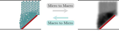
Figure 1 illustrates the switching directions, i.e. from the microscopic to the macroscopic scale and vice versa. For the switch from the microscopic to the macroscopic representation, the idea is to place a Gaussian bell curve corresponding to the mass of each object. The total sum of all curves then leads to a density distribution with high density in dense regions and low density in regions, where the objects are widely spread. The transformation from the macroscopic to the microscopic scale is more involved since the precise positioning is in general not possible. In order to have the objects placed as dense as possible in regions of high density, the idea is to fill the geometry completely and to remove objects according to the density distribution. Therefore, the density is interpreted as a probability density and a nonlinear least squares problem is solved to meet the given density distribution as best as possible. An update algorithm ensures that the objects do not overlap and the placement is admissible.

Figure 1. Idea of the switch: from microscopic to macroscopic scale and vice versa.

The article is organized as follows. Section 1 is concerned with the general description of multi-scale models. The model equations are presented and embedded into the context of hybrid switching. In Section 2, the model switch is applied to a material flow model (Göttlich et al., 2014) and a pedestrian model (Helbing et al., 2000). Section 3 deals with the implementation of the multi-scale model and the hybrid switching algorithm. Finally, in Section 4, numerical examples are analyzed to evaluate the accuracy of the switching method.

2. Multi-scale models

In this section, we present the microscopic and macroscopic scale of the hybrid multi-scale model in a general framework as well as the transition between the levels. Furthermore, the switching idea is introduced based on some key characteristics.

Multi-scale models are commonly used to simulate the evolution of objects over time under certain conditions and inside a given geometry. However, assuming a high number of objects, there might be scenarios, where statistical values of the averaged behavior of objects such as flow (objects per time) or density (objects per area) are sufficient (see e.g. (Colombo et al., 2012; Göttlich et al., 2014)). The general multi-scale model considered here consists of two simulation levels: a microscopic one, described by Newton’s equations of motion, and a macroscopic one relying on a hyperbolic conservation law in two space dimensions (Bellomo et al., 2012; Göttlich, Klar, & Tiwari, 2015).

The setting we are interested in are bounded domains with time-independent external forces. The latter can be exerted for example by the boundaries of the geometry, the friction of a conveyor belt (see Section 2.1) or a desired velocity for pedestrians (see Section 2.2). Other external forces (e.g. gravitational forces) are also possible. The objects are assumed to be uniform and indistinguishable, meaning that they have the same mass, shape and set of parameters. They are assumed to be incompressible and are not allowed to overlap.

2.1. From microscopic to macroscopic scale

The microscopic model is based on Newton’s equations of motion (e.g. (Bellomo et al., 2012)). Being $N$ the number of objects in the system, ${\mathit{x}}_i\in {\mathbb{R}}^2,i=1,\dots ,N$ the spatial coordinate, $\mathit{v}{ }_i\in {\mathbb{R}}^2$ the velocity of object $i$ and $m$ the mass of a single object, the equations are characterized by

(1.1a) $\frac{d\mathit{x}{ }_i}{dt}={\mathit{v}}_i$(1.1a)

(1.1b) $m\frac{d\mathit{v}{ }_i}{dt}=\sum _{i\ne j}\mathit{F}(\mathit{x}{ }_i-\mathit{x}{ }_j,\mathit{v}{ }_i-\mathit{v}{ }_j)+\mathit{G}(x_i,\mathit{v}{ }_i)$(1.1b)

together with an initial condition

(1.2) ${\mathit{x}}_i(0)={\mathit{x}}_{i,0},{\mathit{v}}_i(0)={\mathit{v}}_{i,0}.$(1.2)

Equation (1.1a) describes the velocity of the objects and Equation (1.1b) includes all forces influencing their acceleration. The force term $\mathit{F}:{\mathbb{R}}^2\times {\mathbb{R}}^2\to {\mathbb{R}}^2$ collects the interaction forces, whereas the force term $\mathit{G}:{\mathbb{R}}^2\times {\mathbb{R}}^2\to {\mathbb{R}}^2$ describes exterior forces as for example interactions with boundaries or friction forces.

To derive the limiting macroscopic equations of (1.1), the following formal computations have to be done. We refer to Carrillo et al. (2009); Etikyala et al. (2014); Göttlich et al. (2015); Ruzhansky, Cho, Agarwal, & Area (2017) where such considerations are made for swarming, pedestrian and material flow models in a more detailed way.

We start with the Liouville equation

${\mathrm{\partial }}_t{f}^{(N)}+\hspace{0.17em}\sum _{\mathrm{i}=1}^{\mathrm{N}}\left(\mathrm{d}\mathrm{i}{\mathrm{v}}_{{\mathrm{x}}_{\mathrm{i}}}({\stackrel{.}{\mathrm{x}}}_{\mathrm{i}}{\mathrm{f}}^{(\mathrm{N})})+\mathrm{d}\mathrm{i}{\mathrm{v}}_{{\mathrm{v}}_{\mathrm{i}}}({\stackrel{.}{\mathrm{v}}}_{\mathrm{i}}{\mathrm{f}}^{(\mathrm{N})})\right)=0,$

where $f^{(N)}=f^{(N)}({\mathit{x}}_1,...,{\mathit{x}}_N,{\mathit{v}}_1,...,{\mathit{v}}_N)$ describes the distribution function in the phase space. We integrate over $d{\mathrm{\Omega }}_1=d{\mathit{x}}_2\cdots d{\mathit{x}}_N\times d{v}_2\cdots d{\mathit{v}}_N$ and make use of Equation (1.1b). We consider the chaos assumption $f^{(2)}({\mathit{x}}_1,{\mathit{v}}_1,{\mathit{x}}_2,{\mathit{v}}_2)=f^{(1)}({\mathit{x}}_1,{\mathit{v}}_1)f^{(2)}({\mathit{x}}_2,{\mathit{v}}_2)$, set ${\mathit{F}}_{12}=\mathit{F}({\mathit{x}}_1-{\mathit{x}}_2,{\mathit{v}}_1-{\mathit{v}}_2)$ and let $N$ go to infinity, then the resulting equation for the distribution function $f(\mathit{x},v,t)$ is the mean field equation

(1.3) ${\mathrm{\partial }}_{t}f+\mathit{v}\cdot {\mathrm{\nabla }}_{x}f+Sf=0$(1.3)

with

$Sf=\frac{1}{m}{\mathrm{\nabla }}_v\cdot \left(\int \int \mathit{F}(x-y,v-w)f(\mathit{y}\mathbf{,}\mathit{w})d\mathit{y}d\mathit{w}f(\mathit{x},v)\right)+\frac{1}{m}{\mathrm{\nabla }}_v\cdot (\mathit{G}(\mathit{x},v)f(\mathit{x},v)).$

We define the density

$\rho (\mathit{x},t)=\int f(\mathit{x},v,t)d\mathit{v}$

and velocity

$\mathit{u}(\mathit{x},t)=\frac{\int \mathit{v}f(\mathit{x},\mathit{v},t)d\mathit{v}}{\int f(\mathit{x},\mathit{v},t)d\mathit{v}}.$

Then, the temporal derivative of the density $\rho$ leads to the continuity equation

(1.4) ${\mathrm{\partial }}_t\rho +{\mathrm{\nabla }}_x\cdot (\rho \mathit{u})=0$(1.4)

and the computation of the temporal derivative of $\rho \mathit{u}$ yields the momentum equation

(1.5) $\begin{array}{cc}{\mathrm{\partial }}_t\mathit{u}& +\frac{1}{\rho }\mathit{u}{\mathrm{\nabla }}_{\mathbf{x}}(\rho \mathit{u})+\frac{1}{\rho }{\mathrm{\nabla }}_{\mathbf{x}}\int \mathit{v}\otimes \mathit{v}fd\mathit{v}\\ \hspace{0.17em}& =\frac{1}{\rho }\int \left(+\frac{1}{m}\int \int \mathit{F}\mathbf{(}x-y,v-w)f\mathbf{(}y,w)d\mathit{y}d\mathit{w}+\frac{1}{m}\mathit{G}(x,v)\right)f\mathbf{(}x,v)d\mathit{v}.\end{array}$(1.5)

A monokinetic closure function

$f\sim \rho (\mathit{x},t){\delta }_{u(x,t)}(\mathit{v}(t))$

is used to close the system, i.e. fluctuations are neglected. Moreover, we ignore the velocity dependence meaning that the elastic normal forces dominate the friction forces. So Equation (1.5) reduces to the hydrodynamic limit equation

(1.6) ${\mathrm{\partial }}_{t}u+\frac{1}{\rho }u{\mathrm{\nabla }}_x(\rho u)+\frac{1}{\rho }{\mathrm{\nabla }}_x\int (u\otimes u\cdot \rho )dv=\frac{1}{m}(F^{\ast }\rho )(x)+\frac{1}{m}G(x,u)$(1.6)

which describes the system together with the continuity Equation (1.4).

To reduce the system to a scalar limit equation, a quasi-stationary approach is considered, where the temporal and spatial derivatives are set to zero. We get

$\mathit{G}(x,u)=-({\mathit{F}}^{\ast }\rho )(\mathit{x}).$

If the forces F and G are known, we get an expression for $\mathbf{u}$, the so-called closure velocity (analogous to (Göttlich, Knapp, & Schillen, 2017)) that is of the form

(1.7) ${\mathit{u}}^{\ast }={\mathit{u}}^{\ast }(\rho ,\mathit{x})=\mathit{f}(\rho )\mathbf{(}x)+\mathit{g}(x),$(1.7)

where the first part depends explicitly on the density $\rho$ and the second term only depends on the spatial variable x. We plug the closure velocity ${\mathit{u}}^{\ast }$ into the continuity Equation (1.4) to get the scalar limit equation

(1.8) ${\mathrm{\partial }}_t\rho +{\mathrm{\nabla }}_x\cdot (\rho (f(\rho )+g(x)))=0$(1.8)

which defines the macroscopic model.

The macroscopic model is obviously given by a hyperbolic conservation law in two space dimensions (Aggarwal, Colombo, & Goatin, 2015). The density distribution is denoted by $\rho (\mathit{x},t)$ with spatial coordinate $\mathit{x}\in {\mathbb{R}}^2$ and time variable $t\in {\mathbb{R}}^{+}$. The velocity function corresponds to the closure velocity (1.7).

Note that the model is nonlocal since ${\mathit{u}}^{\ast }(\rho ,\mathit{x})$ does not only depend on $\rho (\mathit{x})$ but on the density distribution $\rho$ over the whole geometry. The boundaries of the domain are denoted by $\mathrm{\partial }{\mathrm{\Omega }}_W$ and the inner normal vector is called $\mathit{n}(x)$. The model Equation (1.8) together with the closure velocity (1.7) and additional initial and boundary conditions can be expressed as follows:

(1.9a) ${\mathrm{\partial }}_t\rho +{\mathrm{\nabla }}_x\cdot (\rho {\mathit{u}}^{\ast }(\rho ,\mathit{x}))=0$(1.9a)

(1.9b) $\rho (\mathit{x},0)={\rho }^0(\mathit{x}),x\in {\mathbb{R}}^2$(1.9b)

(1.9c) $\rho (\mathit{x},t)=0\mathit{x}\in \mathrm{\partial }{\mathrm{\Omega }}_{\mathrm{i}\mathrm{n}\mathrm{f}\mathrm{l}\mathrm{o}\mathrm{w}}$(1.9c)

(1.9d) $⟨{\mathit{u}}^{\ast }(\rho ,\mathit{x}),\mathit{n}(x)⟩=0,\mathit{x}\in \mathrm{\partial }{\mathrm{\Omega }}_W.$(1.9d)

Equation (1.9a) describes evolution of density governed by the hyperbolic conservation law, see Equation (1.8). The initial data is given by (1.9b), the inflow condition is stated by (1.9c) and the condition that no mass is going through the boundaries is ensured by (1.9d).

2.2. Hybrid switching method

The goal of the hybrid switching method is to provide a computational framework to change the scale from the microscopic description (1.1) to the macroscopic (1.9) and vice versa. The switch is directly based on the Eulerian representation, contrary to the situation considered in (Herty & Moutari, 2009; Moutari & Rascle, 2007), and works for a priori defined fixed points in time.

As one might imagine, the transformation from the microscopic to the macroscopic level is straightforward since all necessary information is available. Averaged quantities such as density or flux can be computed in a straightforward way and are sufficient to describe the approximate behavior of the system over time. However, the lack of missing information is the more challenging problem while transforming the system back. Therefore, the main task is to find a method to place the objects inside a given domain such that the given density distribution matches the position of objects in the microscopic scale. For application purposes, the transformation from the macroscopic to the microscopic representation is necessary whenever the trajectory of single objects is needed.

The consistent relation between the amount of mass and the number of objects is ensured by

(1.10) $m_{\mathrm{t}\mathrm{o}\mathrm{t}}=N\cdot 2\sqrt{3}{r}^2\cdot {\rho }_{\mathrm{m}\mathrm{a}\mathrm{x}}$(1.10)

with $m_{\mathrm{t}\mathrm{o}\mathrm{t}}$ being the total mass in the system, $r$ the radius of an object and $N$ again the total number of objects. Note that this number is independent on the switching direction and the derivation is as follows: If we have a domain of maximal density ${\rho }_{\mathrm{m}\mathrm{a}\mathrm{x}}$, the corresponding object distribution is as dense as possible which is a hexagonal configuration (Degond, Ferreira, & Motsch, 2017). Then, the volume corresponding to one object corresponds the volume of a hexagon with inner circle radius $r$. The area of such an hexagon is $A_{\mathrm{h}\mathrm{e}\mathrm{x}}=2\sqrt{3}{r}^2$. The volume for one object therefore is

(1.11) $V_{\mathrm{o}\mathrm{b}\mathrm{j}\mathrm{e}\mathrm{c}\mathrm{t}}=A_{\mathrm{h}\mathrm{e}\mathrm{x}}\cdot {\rho }_{\mathrm{m}\mathrm{a}\mathrm{x}}=2\sqrt{3}{r}^2\cdot {\rho }_{\mathrm{m}\mathrm{a}\mathrm{x}}.$(1.11)

2.3. Switch from microscopic to macroscopic scale

The transformation from the microscopic to the macroscopic representation is performed such that the original position of objects can be interpreted as a density distribution. Thus, the idea is to spend a two-dimensional Gaussian bell curve for each object representing the density distribution and sum them all up. Since the volume of a two-dimensional Gaussian function with variance ${\sigma }_0$ is normalized and the volume per object has to be equal to $V_{\mathrm{o}\mathrm{b}\mathrm{j}\mathrm{e}\mathrm{c}\mathrm{t}}$, we have to multiply by the corresponding volume as done in Equation (1.11). The $x$- resp. $y$-coordinates of the objects are given by the vectors $X_o$ and $Y_o$ and the continuous density distribution for one object $i$ is then

(1.12) $D_i(x,y)=\frac{1}{{\rho }_{\mathrm{m}\mathrm{a}\mathrm{x}}2\pi {\sigma }_0^2}exp\left(\frac{-1}{2{\sigma }_0^2}\left(\parallel x-X_{o,i}{\parallel }_2^2+\parallel y-Y_{o,i}{\parallel }_2^2\right)\right)\cdot V_{\mathrm{o}\mathrm{b}\mathrm{j}\mathrm{e}\mathrm{c}\mathrm{t}},$(1.12)

where $X_{o,i}$ and $Y_{o,i}$ is the $i$-th component of the vector $X_o$ and $Y_o$, respectively. Summing the densities for each object

(1.13) $\rho (x,y)=\sum _{i=1}^N{D}_i(x,y),$(1.13)

we end up with the desired continuous density distribution.

2.4. Switch from macroscopic to microscopic scale

The switch becomes more involved when the system is transformed from the macroscopic to the microscopic representation. This is due to missing detailed information on individual objects at the macroscopic level. To remedy this drawback, we need to solve an optimization problem to find a good guess for the microscopic density interpretation. To do so, the density distribution is considered as a normalized probability distribution, meaning that the maximal density is ${\rho }_{\mathrm{m}\mathrm{a}\mathrm{x}}=1.$ Since it is not possible to compare the placement of objects to the macroscopic density distribution ${\rho }_{\mathrm{m}\mathrm{a}\mathrm{c}}$, the object distribution has to be transformed back to a density distribution called ${\rho }_{\mathrm{a}\mathrm{p}\mathrm{p}}$, cf. (1.13). Given the position of objects $\left\{X_o,Y_o\right\}$ respecting the boundaries and the non-overlapping conditions, we can set up an optimization problem of the following form:

(1.14a) $min\parallel {\rho }_{\mathrm{m}\mathrm{a}\mathrm{c}}-{\rho }_{\mathrm{a}\mathrm{p}\mathrm{p}}{\parallel }_2^2$(1.14a)

(1.13) $\mathrm{w}\mathrm{i}\mathrm{t}\mathrm{h}{\rho }_{\mathrm{a}\mathrm{p}\mathrm{p}}\approx \rho (x,y)=\sum _{i=1}^N{D}_i(x,y)\mathrm{a}\mathrm{s}\mathrm{i}\mathrm{n}\mathrm{e}\mathrm{q}\mathrm{u}\mathrm{a}\mathrm{t}\mathrm{i}\mathrm{o}\mathrm{n}$(1.13)

(1.14b) $\mathrm{s}.\mathrm{t}.\mathrm{\#}\mathrm{o}\mathrm{b}\mathrm{j}\mathrm{e}\mathrm{c}\mathrm{t}\mathrm{s}=N$(1.14b)

(1.14c) $(X_{o,i},Y_{o,i})\in {\mathrm{\Omega }}_{\mathrm{a}\mathrm{d}}\mathrm{\forall }i\in \left\{1,\dots ,N\right\}$(1.14c)

(1.14d) $\sqrt{{(X_{o,i}-X_{o,j})}^2+{(Y_{o,i}-Y_{o,j})}^2}>2r\mathrm{\forall }i,j\in \left\{1,\dots ,N\right\},i\ne j,$(1.14d)

where ${\mathrm{\Omega }}_{\mathrm{a}\mathrm{d}}$ is the admissible interior domain such that objects placed here do not interact with the boundaries. The optimization problem (1.14) is in fact a nonlinear least squares problem subject to the constraints that the total numbers of objects is met (1.14b), the objects are placed inside the admissible domain (1.14c) and do not overlap (1.14d). For the numerical implementation, the constraints (1.14c) and (1.14d) are ensured by an update algorithm and are not considered directly in the solution of the optimization problem.

A crucial point is to find an admissible start solution ${\rho }_{\mathrm{a}\mathrm{p}\mathrm{p}}.$ Therefore, we require that high-density regions, where ${\rho }_{\mathrm{m}\mathrm{a}\mathrm{x}}$ is attained, are packed as dense as possible such that the geometry is filled completely and then remove objects until the number $N=\frac{m_{\mathrm{t}\mathrm{o}\mathrm{t}}}{V_{\mathrm{o}\mathrm{b}\mathrm{j}\mathrm{e}\mathrm{c}\mathrm{t}}}$ is reached. First, objects, where the density is lower than a certain tolerance value $ϵ$, are removed. For any other placement, remove the object with a probability of $(1-\rho (x))$, where $x$ is the center of the corresponding object. This means that in each possible position, the objects are placed in a Bernoulli distributed way with probability equal to the density. In general, the number of objects is not equal to $N$ after this procedure. So if the number of objects is too large, remove objects in low density regions. Otherwise, if the number of objects is too low, refill positions in high-density regions.

Further details on the numerical solution of (1.14) and the update algorithm can be found in sub section 3.1.

In the next section, we present two applications to demonstrate the switching idea. They mainly differ in the evaluation of the force terms in particular the exterior forces.

3. Applications

3.1. Material flow model

We briefly introduce the microscopic and macroscopic material flow model. The models are described in detail in Göttlich et al. (2014, 2015) and the formal derivation of the macroscopic via the hydrodynamic limit is given in Göttlich et al. (2015).

3.2. Microscopic model

In the considered application case, circular-shaped parts of radius $r$ are transported on a conveyor belt. The arising exterior forces are the interaction forces between parts and boundaries as well as the friction force induced by the conveyor belt. Analogous to Göttlich et al. (2015), we have to specify the force terms in (1.1) as F being the interaction force between the parts and G the friction force of the belt combined with wall forces. The interaction force F in Equation (1.1b) can be split into a tangential part $f^t$ and a normal part $f^n$:

(2.1) $F(\mathit{x},\mathit{v})=H(2r-\parallel \mathit{x}\parallel )\cdot (f^n(\mathit{x},\mathit{v})+f^t(\mathit{x},\mathit{v})),$(2.1)

where $H$ denotes the common Heaviside function with $H(\cdot )=1$ if $\parallel \mathit{x}\parallel <2r$ and $0$ otherwise. The normal force component itself can be split into an elastic repulsive part $f_{el}^n$ and a dissipative part $f_{diss}^n$:

$f^n(\mathit{x},\mathit{v})=\underset{=f_{el}^n}{\underbrace{k_n\cdot \frac{\mathit{x}}{\parallel \mathit{x}\parallel }\cdot (2r-\parallel \mathit{x}\parallel )}}-\underset{=f_{diss}^n}{\underbrace{{\gamma }_n⟨v,\frac{\mathit{x}}{\parallel \mathit{x}\parallel }⟩\frac{\mathit{x}}{\parallel \mathit{x}\parallel }}}.$

The repulsive force is modeled by a spring damper model with the normal spring constant $k_n$ while the dissipative force is equipped with the normal viscous coefficient ${\gamma }_n$. The tangential force is given by

$f^t(\mathit{x},\mathit{v})=-min({\gamma }_t\parallel {\mathit{v}}^t\parallel ,\mu \parallel f^n\parallel )\cdot \frac{{\mathit{v}}^t}{\parallel {\mathit{v}}^t\parallel }$

with Coulomb friction coefficient $\mu$ and tangential viscous damping coefficient ${\gamma }_t$. The tangential velocity ${\mathit{v}}^t$ is

${\mathit{v}}^t=\mathit{v}-⟨\mathit{v},\mathit{n}⟩\mathit{n}.$

The friction force $f_{fric}$ describes the interaction between a part and the surface of the conveyor belt

$f_{fric}({\mathit{v}}_i)=-min({\mu }_b\cdot m\cdot g,{\gamma }_b\cdot \parallel {\mathit{v}}_i-{\mathit{v}}_T\parallel )\cdot \frac{{\mathit{v}}_i-{\mathit{v}}_T}{\parallel {\mathit{v}}_i-{\mathit{v}}_T\parallel }$

with constant positive velocity of the conveyor belt $v_T$, part mass $m$ and gravitational constant $g$. The bottom friction coefficient ${\mu }_b$ and the bottom viscous damping coefficient ${\gamma }_b$ depend on the material of the belt and of the parts.

The interaction force between the parts and the boundaries of the conveyor belt are modeled in the same way as the interaction force of the parts. The set containing the indices of walls and boundaries is called $W$.

The exterior forces are the sum of the interaction forces with the boundaries and the friction forces between the parts and the conveyor belt

(2.2) $\mathit{G}(x_i,v_i)=\sum _{w\in W}H(r-\mathrm{d}\mathrm{i}\mathrm{s}\mathrm{t}(x_i,w))\cdot (f_{w,i}^n+f_{w,i}^t)+f_{fric}({\mathit{v}}_i)$(2.2)

with $f_{w,i}^n$ and $f_{w,i}^t$ the normal and tangential forces exerted by the walls on part $i$.

The complete microscopic material flow model is obtained by inserting these force terms into the general microscopic model (1.1) and reads

(2.3a) $\frac{d\mathit{x}{ }_i}{dt}=\mathit{v}{ }_i$(2.3a)

(2.3b) $m\frac{d{v}_i}{dt}=\sum _{i\ne j}F({\mathit{x}}_i-{\mathit{x}}_j,{\mathit{v}}_i-{\mathit{v}}_j)+\mathbf{G}({\mathit{x}}_i,{\mathit{v}}_i)$(2.3b)

with F and G as in (2.1), (2.2) and initial conditions ${\mathit{x}}_i(0)={\mathit{x}}_{i,0},{\mathit{v}}_i(0)={\mathit{v}}_{i,0}$.

3.3. Macroscopic model

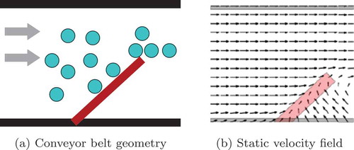
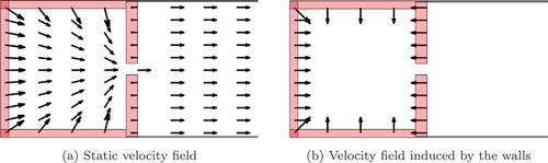
The static space-dependent velocity $\mathit{g}(x)$ in Equation (1.7) represents the friction force of the conveyor belt and the force exerted by the boundaries of the given setting, see Figure 2a. The resulting velocity field is shown in Figure 2b. The dynamic velocity $\mathit{f}(\rho )$ is needed to deal with situations of maximal density ${\rho }_{\mathrm{m}\mathrm{a}\mathrm{x}}$.

Figure 2. Sketch of the conveyor belt.

For the formulation of the macroscopic model as in (1.9a) we set

(2.4) $f(\rho )={\mathit{v}}^{\mathrm{d}\mathrm{y}\mathrm{n}}(\rho ),\mathit{g}(\mathit{x})={\mathit{v}}^{\mathrm{s}\mathrm{t}\mathrm{a}\mathrm{t}}(\mathit{x}),$(2.4)

where the static velocity field ${\mathit{v}}^{\mathrm{s}\mathrm{t}\mathrm{a}\mathrm{t}}$ is as in Figure 2b. The nonlocal dynamic vector field ${\mathit{v}}^{\mathrm{d}\mathrm{y}\mathrm{n}}$ should be active if the density exceeds a maximal density ${\rho }_{\mathrm{m}\mathrm{a}\mathrm{x}}$ and parts start to pile up. Below the maximal density, ${\mathit{v}}^{\mathrm{d}\mathrm{y}\mathrm{n}}$ is inactive, i.e. free flow regime, and the parts are transported with the velocity given by ${\mathit{v}}^{stat}$. Thus, the dynamic vector field includes the interaction between parts weighted by the factor $ϵ>0$ and models the formation of congestion in front of an obstacle by the collision operator $\mathbf{I}(\rho )$:

(2.5) $v^{\mathrm{d}\mathrm{y}\mathrm{n}}(\rho )=H(\rho -{\rho }_{\mathrm{m}\mathrm{a}\mathrm{x}})\cdot \mathbf{I}(\rho ),$(2.5)

where $H$ denotes the common Heaviside function and

(2.6) $\mathbf{I}(\rho )=-ϵ\frac{\mathrm{\nabla }({\eta }^{\ast }\rho )}{\sqrt{1+\parallel \mathrm{\nabla }({\eta }^{\ast }\rho ){\parallel }_2^2}}.$(2.6)

The negative of the gradient of the convolution means that if there is a pile of maximal density, the mass will be pushed in a region with lower density. Inside a pile with maximal density, this force will be zero. Additionally, we have the initial condition

(2.7) $\rho (\mathit{x},0)={\rho }^0(\mathit{x}),x\in {\mathbb{R}}^2$(2.7)

and the boundary condition

$⟨{\mathit{u}}^{\ast }(x,\rho ),\mathit{n}(x)⟩=0,\mathit{x}\in \mathrm{\partial }{\mathrm{\Omega }}_W.$

The computational domain is denoted by $\mathrm{\Omega }$ and the boundaries are $\mathrm{\partial }\mathrm{\Omega }$. The inflow boundary at the left in Figure 2 is called $\mathrm{\partial }{\mathrm{\Omega }}_{\mathrm{i}\mathrm{n}\mathrm{f}\mathrm{l}\mathrm{o}\mathrm{w}}$. The walls and the obstacle are denoted by $\mathrm{\partial }{\mathrm{\Omega }}_W$, even if the obstacle is not at the boundary of the computational domain. The normal vector is called n(x).

The complete macroscopic material flow model is obtained by inserting the velocity components (2.4) into the closure velocity (1.7). Then, the analogon to system (1.9) reads as follows (see (Göttlich et al., 2014)):

(2.8a) ${\mathrm{\partial }}_t\rho +{\mathrm{\nabla }}_x\cdot (\rho ({\mathit{v}}^{\mathrm{d}\mathrm{y}\mathrm{n}}(\rho )+{\mathit{v}}^{\mathrm{s}\mathrm{t}\mathrm{a}\mathrm{t}}(\mathit{x})))=0$(2.8a)

(2.8b) ${\mathit{v}}^{\mathrm{d}\mathrm{y}\mathrm{n}}(\rho )=H(\rho -{\rho }_{max})\cdot \mathbf{I}(\rho )$(2.8b)

(2.8c) $\mathbf{I}(\rho )=-ϵ\frac{\mathrm{\nabla }({\eta }^{\ast }\rho )}{\sqrt{1+\parallel \mathrm{\nabla }(\eta \ast \rho ){\parallel }_2^2}}$(2.8c)

(2.8d) $\rho (\mathit{x},0)={\rho }^0(\mathit{x}),x\in {\mathbb{R}}^2$(2.8d)

$\rho (\mathit{x},t)=0\mathit{x}\in \mathrm{\partial }{\mathrm{\Omega }}_{\mathrm{i}\mathrm{n}\mathrm{f}\mathrm{l}\mathrm{o}\mathrm{w}}(2.8e)$

(2.8f) $⟨{\mathit{v}}^{\mathrm{d}\mathrm{y}\mathrm{n}}(\rho )+{\mathit{v}}^{\mathrm{s}\mathrm{t}\mathrm{a}\mathrm{t}}(\mathit{x}),\mathit{n}(\mathit{x})⟩=0,\mathit{x}\in \mathrm{\partial }{\mathrm{\Omega }}_W.$(2.8f)

3.4. Pedestrian flow model

3.4.1. Microscopic model

In the following sections, the pedestrian model derived by Helbing (Helbing et al., 2000) is briefly reviewed and a corresponding macroscopic model is stated. We assume the pedestrians to be of circular shape with radius $r$ and to act in the same way in each direction, meaning that the forces are rotationally invariant. We specify again the force terms F for the interaction and G for the desired velocity of pedestrians as well as the forces exerted by the walls. We set ${\mathit{F}}_{ij}$ to characterize the interaction force between pedestrian $i$ and $j$ in (1.1b). The latter is modeled as

$F({\mathit{x}}_i-{\mathit{x}}_j,{\mathit{v}}_i-{\mathit{v}}_j)=F_{ij}=\left(Aexp\left(\frac{(2r-d_{ij})}{B}\right)+k\cdot h(2r-d_{ij})\right){\mathit{n}}_{ij}+\kappa \cdot h(2r-d_{ij})\mathrm{\Delta }{v}_{ji}^{\mathit{t}}{\mathit{t}}_{ij}$

with $h(y)=H(y)\cdot y$ and $H$ the Heaviside function. The constants $A,B,k$ are positive, whereas $\kappa$ can be equal to zero if tangential force effects are neglected. The distance of pedestrians $i$ and $j$ is given by $d_{ij}=\parallel {\mathit{x}}_i-{\mathit{x}}_j\parallel$ with $x_i$ and $x_j$ the centers of mass, ${\mathit{n}}_{ij}=({\mathit{x}}_i-{\mathit{x}}_j)/d_{ij}$ is the normalized vector pointing from pedestrian $j$ to pedestrian $i$, ${\mathit{t}}_{ij}=(-n_{ij}^{(2)},n_{ij}^{(1)})$ is the tangential direction and $\mathrm{\Delta }{v}_{ji}^t=({\mathit{v}}_j-{\mathit{v}}_i)\cdot {\mathit{t}}_{ij}$.

The interaction force ${\mathit{F}}_{iw}$ between wall $w\in W$ and pedestrian $i$ is modeled as

(2.9) ${\mathit{F}}_{iw}=\left(Aexp\left(\frac{(r-d_{iw})}{B}\right)+k\cdot h(r-d_{iw})\right){\mathit{n}}_{iw}-\kappa \cdot h(r-d_{iw})({\mathit{v}}_i\cdot {\mathit{t}}_{iw}){\mathit{t}}_{iw}$(2.9)

with $d_{iw}$ being the distance of pedestrian $i$ to wall $w$, ${\mathit{n}}_{iw}$ the normalized normal vector of wall $w$ and ${\mathit{t}}_{iw}$ the tangential vector of wall $w$. Combined with the component of the desired velocity

${\mathit{v}}^{\mathrm{d}\mathrm{e}\mathrm{s}}({\mathit{x}}_i)=\frac{{\mathit{v}}^0({\mathit{x}}_i)-\mathit{v}({\mathit{x}}_i)}{\tau },$

where $\tau$ is the reaction time and ${\mathit{v}}^0(\mathit{x})$ is the desired velocity depending on the pedestrians location, we set the exterior force as

$\mathit{G}({\mathit{x}}_i,{\mathit{v}}_i)=m{\mathit{v}}^{\mathrm{d}\mathrm{e}\mathrm{s}}({\mathit{x}}_i)+F_{iW}({\mathit{x}}_i,{\mathit{v}}_i).$

Compared to the material flow model, where the main ingredient is the friction of the conveyor belt, the exterior force for the pedestrian model is mainly driven by the desired velocity of pedestrians. Note that this leads to a different numerical treatment within the switching algorithm. Inserting these terms into the system (1.1), we have the scaled microscopic pedestrian model

(2.10a) $\frac{d\mathit{x}{ }_i}{dt}={\mathit{v}}_i$(2.10a)

(2.10b) $m\frac{d\mathit{v}{ }_i}{dt}=m{\mathit{v}}_i^{des}+\frac{1}{N}\sum _{j\ne i}{F}_{ij}+\frac{1}{N}\sum _W{F}_{iW}$(2.10b)

with initial positions ${\mathit{x}}_i(0)={\mathit{x}}_{i,0}$ and velocities ${\mathit{v}}_i(0)={\mathit{v}}_{i,0}$.

3.4.2. Macroscopic model

For the macroscopic pedestrian model, we have to determine the parts of the velocity ${\mathit{u}}^{\ast }(\rho ,\mathit{x})=f(\rho )(\mathit{x})+\mathit{g}(\mathit{x})$, see (1.7), as

$\mathit{f}(\rho )=\frac{1}{m\lambda }{\mathit{F}}^{\ast }\rho ,\mathit{g}(x)={\mathit{v}}^0(\mathit{x})+\frac{1}{m\lambda }\sum _W{\mathit{F}}_W(\mathit{x})$

with

(2.11) $\begin{array}{cc}\left(F^{\ast }\rho \right)(x)& =\int \mathit{F}\mathbf{(}\mathit{x}\mathbf{-}\mathit{y}\mathbf{)}\rho (\mathit{y})d\mathit{y}\\ \hspace{0.17em}& =\int \left(Aexp\left(\frac{2r-\parallel \mathit{x}\mathbf{-}\mathit{y}\parallel }{B}\right)+kh(2r-\parallel x-y\parallel )\right)\frac{\mathit{x}\mathbf{-}\mathit{y}}{\parallel \mathit{x}\mathbf{-}\mathit{y}\parallel }\rho (\mathit{y})d\mathit{y},\end{array}$(2.11)

${\mathit{v}}^0(\mathit{x})$ is the desired velocity depending on the pedestrians location and

$\sum _W{\mathit{F}}_W(\mathit{x})=\sum _W\left(A\mathit{x}p\left(\frac{r-d(\mathit{x})}{B}\right)+kh(r-d(\mathit{x}))\right){\mathit{n}}_W,$

where $h$ is defined before. The constants $A,B,k$ and the radius of the pedestrians $r$ are the same as in the microscopic model. Here, $d(x)$ denotes the distance of x and the interacting wall.

The complete macroscopic pedestrian model then reads as

(2.12a) ${\mathrm{\partial }}_t\rho +{\mathrm{\nabla }}_{\mathit{x}}\cdot \left[\rho \left({\mathit{v}}^0(\mathit{x})+\frac{1}{m\lambda }\mathit{F}\ast \rho (\mathit{x})+\frac{1}{m\lambda }\sum _W{\mathit{F}}_W(\mathit{x})\right)\right]=0$(2.12a)

(2.12b) $\rho (\mathit{x},0)={\rho }^0(\mathit{x}),\mathit{x}\in {\mathbb{R}}^2$(2.12b)

(2.12c) $\rho (x,t)=0x\in \mathrm{\partial }{\mathrm{\Omega }}_{\mathrm{i}\mathrm{n}\mathrm{f}\mathrm{l}\mathrm{o}\mathrm{w}}$(2.12c)

(2.12d) $⟨{\mathit{u}}^{\ast }(\rho ,\mathit{x}),\mathit{n}(\mathit{x})⟩=0,\mathit{x}\in \mathrm{\partial }{\mathrm{\Omega }}_W.$(2.12d)

with Equation (2.12b) the initial condition, (2.12c) specifying the inflow condition and (2.12d) the boundary condition.

4. Numerical discretization

In this section, the numerical discretization of the microscopic (1.1) and the macroscopic model (1.9) are presented. The discretized models are then used to set up the hybrid switching method introduced in subsection 1.2.

We set $dt$ the time step of the discretization. The discretized microscopic model reads

(3.1a) $\frac{{\mathit{x}}_i(t+dt)-{\mathit{x}}_i(t)}{dt}={\mathit{v}}_i(t)$(3.1a)

(3.1b) $m\frac{{\mathit{v}}_i(t+dt)-{\mathit{v}}_i(t)}{dt}=\sum \mathit{F}({\mathit{x}}_i(t)-{\mathit{x}}_j(t),{\mathit{v}}_i(t)-v_j(t))+\mathit{G}({\mathit{x}}_i(t),{\mathit{v}}_i(t))$(3.1b)

together with the initial condition

${\mathit{x}}_i(0)={\mathit{x}}_{i,0},{\mathit{v}}_i(0)={\mathit{v}}_{i,0}.$

It is solved via a classical Runge-Kutta method of fourth order. If the specific application is known, a priori estimates can be performed for the force terms F and G. Then, the time step can be chosen appropriately and the need of an adaptation of the step size during the computation can be avoided.

For the discretization of the macroscopic model we denote by $\mathrm{\Delta }{x}_1$, $\mathrm{\Delta }{x}_2$ the space step sizes and $\mathrm{\Delta }t$ the time step size. The grid points are defined as

(3.2) $x_i^{(1)}=i\cdot \mathrm{\Delta }{x}_1,i=1,\dots ,N_{x_1},x_j^{(2)}=j\cdot \mathrm{\Delta }{x}_2,j=1,\dots ,N_{x_2},t^k=k\cdot \mathrm{\Delta }t,k=1,\dots ,N_t.$(3.2)

The space is subdivided into squares $S_{i,j}=\left[x_{i-\frac{1}{2}}^{(1)},x_{i+\frac{1}{2}}^{(1)}]\times [x_{j-\frac{1}{2}}^{(2)},x_{j+\frac{1}{2}}^{(2)}\right]$ with grid constants ${\lambda }^{(d)}=\frac{\mathrm{\Delta }t}{\mathrm{\Delta }{x}_d}$ for $d=1,2$. We apply a finite volume scheme, where the density is considered as a piecewise constant function

$\rho (\mathit{x},t)={\rho }_{i,j}^k\in \mathbb{R}\mathrm{f}\mathrm{o}\mathrm{r}\mathit{x}\in S_{i,j},k\in \left\{1,\dots ,N_t\right\}.$

Due to (1.7), we have that the velocity parts $f(\rho )$ and $g(x)$ only depend on $\rho$ or x, respectively. This allows for a separate numerical computation in terms of the numerical fluxes

(3.3a) $F_{i,j}^{(1),+}=F_{i,j}^{(1)}(\rho ,{\rho }_{i,j}^k,{\rho }_{i+1,j}^k,{\mathit{x}}_{i+\frac{1}{2},j})+G_{i,j}^{(1)}({\rho }_{i,j}^k,{\rho }_{i+1,j}^k,{\mathit{x}}_{i+\frac{1}{2},j})$(3.3a)

(3.3b) $F_{i,j}^{(1),-}=F_{i,j}^{(1)}(\rho ,{\rho }_{i-1,j}^k,{\rho }_{i,j}^k,{\mathit{x}}_{i-\frac{1}{2},j})+G_{i,j}^{(1)}({\rho }_{i-1,j}^k,{\rho }_{i,j}^k,{\mathit{x}}_{i-\frac{1}{2},j})$(3.3b)

(3.3c) $F_{i,j}^{(2),+}=F_{i,j}^{(2)}(\rho ,{\tilde{\rho }}_{i,j}^k,{\tilde{\rho }}_{i,j+1}^k,{\mathit{x}}_{i,j+\frac{1}{2}})+G_{i,j}^{(2)}({\tilde{\rho }}_{i,j}^k,{\tilde{\rho }}_{i,j+1}^k,{\mathit{x}}_{i,j+\frac{1}{2}})$(3.3c)

(3.3d) $F_{i,j}^{(2),-}=F_{i,j}^{(2)}(\rho ,{\tilde{\rho }}_{i,j-1}^k,{\tilde{\rho }}_{i,j}^k,{\mathit{x}}_{i,j-\frac{1}{2}})+G_{i,j}^{(2)}({\tilde{\rho }}_{i,j-1}^k,{\tilde{\rho }}_{i,j}^k,{\mathit{x}}_{i,j-\frac{1}{2}}),$(3.3d)

where the density-dependent part is given by

$F_{i,j}^{(1)}\left(\rho ,{\rho }_{i,j}^k,{\rho }_{i+1,j}^k,{\mathit{x}}_{i+\frac{1}{2},j}\right)=\left\{\begin{array}{cc}{\rho }_{i,j}{f}^{(1)}(\rho )({\mathit{x}}_{i+\frac{1}{2},j})& f^{(1)}(\rho )({\mathit{x}}_{i+\frac{1}{2},j})\ge 0\\ {\rho }_{i+1,j}{f}^{(1)}(\rho )({\mathit{x}}_{i+\frac{1}{2},j})& f^{(1)}(\rho )({\mathit{x}}_{i+\frac{1}{2},j})\le 0\end{array}\right.$

and the position-dependent part is

$G_{i,j}^{(1)}\left({\rho }_{i,j}^k,{\rho }_{i+1,j}^k,{\mathit{x}}_{i+\frac{1}{2},j}\right)=\left\{\begin{array}{cc}{\rho }_{i,j}{g}^{(1)}({\mathit{x}}_{i+\frac{1}{2},j})& g^{(1)}({\mathit{x}}_{i+\frac{1}{2},j})\ge 0\\ {\rho }_{i+1,j}{g}^{(1)}({\mathit{x}}_{i+\frac{1}{2},j})& g^{(1)}({\mathit{x}}_{i+\frac{1}{2},j})\le 0.\end{array}\right.$

We remark that f and g depend on the application we have in mind. In vertical direction, the computation of the numerical fluxes $F_{i,j}^{(2)}$ and $G_{i,j}^{(2)}$ follows analogously.

A dimensional splitting method is used to reduce the original two-dimensional problem into the solution of one-dimensional problems only. The discretized system is then

(3.4a) ${\tilde{\rho }}_{i,j}^k={\rho }_{i,j}^k-{\lambda }^{(1)}[F_{i,j}^{(1),+}-F_{i,j}^{(1),-}]\mathrm{\forall }(i,j)\in \{1,\dots ,N_{x_1}\}\times \{1,...,N_{x_2}\}$(3.4a)

(3.4b) ${\rho }_{i,j}^{k+1}={\tilde{\rho }}_{i,j}^k-{\lambda }^{(2)}[F_{i,j}^{(2),+}-F_{i,j}^{(2),-}]\mathrm{\forall }(i,j)\in \{1,...,N_{x_1}\}\times \{1,...,N_{x_2}\}$(3.4b)

(3.4c) ${\rho }_{i,j}(0)={\rho }_{i,j}^0\mathrm{\forall }(i,j)\in \left\{1,...,N_{x_1}\right\}\times \left\{1,...,N_{x_2}\right\}$(3.4c)

(3.4d) $⟨\mathit{u}(\rho ,{\mathit{x}}_{i,j}),n_{i,j}⟩=0\mathrm{\forall }(i,j)\in W$(3.4d)

with $W$ the set containing the grid points corresponding to the boundaries of the underlying domain. The step sizes have to be chosen such that the CFL condition

(3.5) $\frac{\mathrm{\Delta }t}{\mathrm{\Delta }{x}_d}\underset{\rho }{max}\parallel \frac{\mathrm{\partial }}{\mathrm{\partial }\rho }(\rho (\mathit{f}(\rho )+\mathit{g}\mathbf{(}\mathit{x}\mathbf{)}){\parallel }_{\mathrm{\infty }}\le 1$(3.5)

for $d=1,2$ is fulfilled.

4.1. Hybrid switching algorithms

The numerical discretizations are now used to present an implementation of the hybrid switching method, see subsection 1.2.

4.1.1. Microscopic to macroscopic representation

As we have seen, the given geometry is partitioned into grid cells for the numerical computation. Let us denote by $x_c$ and $y_c$ vectors containing the $x$- resp. $y$-coordinate of the grid cell centers. Corresponding to (1.13), the density in grid cell $i$ can be calculated via

(3.6) ${\rho }_{\mathrm{i}}=\left(\sum _{j=1}^N{D}_j(x_{c,i},y_{c,i}))\right)$(3.6)

with $D_j$ being the density corresponding to object $j$, see Equation (1.12). The variance ${\sigma }_0>0$ has to be chosen such that the numerical support of the bell function is larger than the actual domain of one object, otherwise we obtain peaks for densely packed objects and not a uniform-density distribution. In doing so, the implementation of the microscopic to macroscopic direction is straightforward as expected.

4.1.2. Macroscopic to microscopic representation

The optimization problem (1.14) can be interpreted as a nonlinear least squares problem if the constraints (1.14c) and (1.14d) are omitted (cf. discussion in subsection 1.2) and treated in an additional routine. Therefore, the computation of the macro to micro switching direction can be split into the following steps:

1. Find admissible start solution ${\rho }_{\mathrm{a}\mathrm{p}\mathrm{p}}$: The pseudocode to find an admissible start solution is specified in algorithm 1. The algorithm can be run several times to improve the configuration of the start solution since a random choice of object placement is used.

2. Solve nonlinear least squares problem (1.14a)–(1.14b): The nonlinear least squares problem is solved with the MATLAB function lsqnonlin https://de.mathworks.com/help/optim/ug/lsqnonlin.html and requires the solution $P$ of algorithm 1 as initialization. The numerical solution of the nonlinear least sqaures problem is denoted by $Q$.

3. Solve problem including the constraints (1.14c)–(1.14d): The main idea of the so-called update algorithm 2 is to move the objects $i$ with coordinates $P(i)$ from the optimized solution $Q(i)$ such that they do not overlap any more. This means in particular if object $i$ interacts with object $j\ne i$ or with the wall, i.e. $|S(i)-S(j){|}_2\le 2r,j\ne i$ or $Q(i)\notin {\mathrm{\Omega }}_{\mathrm{a}\mathrm{d}}$, we set $S(i)=(P(i)+S(i))/2$ and check again for interactions until $\left|P(i)-S(i)\right|$ is less than a predefined tolerance $\delta$. The final configuration satisfying (1.14c)–(1.14d) is denoted by $S(i)$.

Algorithm 1 Find admissible start solution

Input: Density ρ_mac, mass m, radius r, # objects N, tolerance $ϵ$, admissible region Ω_ad

Output: Solution P containing the coordinates of the object centers

• 1: Compute a hexagonal grid structure with grid point distance 2r and grid points g_i: = (x_i, y_i)

• 2: for i = 1: # grid points do

• 3: if g_i ∉Ω_ad then

• 4: Delete grid point g_i

• 5: end if

• 6: end for

• 7: for i = 1: # remaining grid points do

• 8: Determine corresponding density value ρi = ρ_mac(x_i, y_i)

• 9: if ρ_i < $ϵ$ then

• 10: Delete grid point i

• 11: else

• 12: Delete grid point i with probability (1 − ρi)

• 13: end if

• 14: end for

• 15: if N > # remaining grid points then

• 16: Put grid point with index argmaxi{ρ_i|g_i has been deleted} until N is met

• 17: else if N < # remaining grid points then

• 18: Delete grid point with index argmini{ρ_i|g_i not deleted} until N is met

• 19: end if

• 20: return Remaining grid points as matrix P corresponding to the placed objects centers

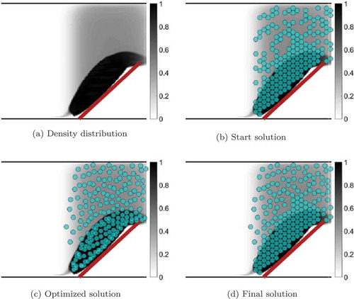
Figure 3 shows a possible evaluation of the update algorithm including a figure for the macroscopic density that should be reproduced, see Figure 3a, a figure for a possible start solution computed by algorithm 1, see Figure 3b, a figure for the optimized solution applying the MATLAB algorithm lsqnonlin, see Figure 3c, where we directly observe that the non-overlap condition is injured, and a figure for the final solution after applying the update algorithm 2, see Figure 3d. Concluding, the latter is a combination of the start and optimized solution. We observe that in regions, where the density is high, the objects are placed as dense as possible, whereas in regions, where the density is far from the maximal density, objects get stuck.

Figure 3. Macroscopic to microscopic representation.

Note that the runtime growths linearly in $N$ for algorithm 1 and the solution of the optimization problem. The runtime for the update algorithm 2 growths cubically in $N$. However, the solution of the optimization problem using MATLAB takes several hours and dominates the performance of the update algorithm for the test cases we present in Section 4.

Algorithm 2 Update algorithm ensuring the non-overlapping condition

Input: Solution Q of least squares problem, start solution P, admissible region Ω_ad, tolerance δ

Output: Final solution S ensuring a placement of the objects without overlapping

• 1: Initialize solution with S = P

• 2: for k = 1: N do

• 3: for i = 1: N do

• 4: interaction = 0

• 5: Place object i at optimized position: S(i) = Q(i)

• 6: if $s(i)\notin {\mathrm{\Omega }}_{ad}$then

• 7: interaction = 1

• 8: end if

• 9: for j = 1: N do

• 10: if |S(i) − S(j)|₂ ≤ 2r, j ≠ i then

• 11: interaction = 1

• 12: end if

• 13: end for

• 14: if interaction = 1 then

• 15: if |P (i) − S(i)| < δ then

• 16: STOP, S(i) = P (i), go back to step 3

• 17: end if

• 18: S(i) = (P (i) + S(i))/2 and go back to step 6

• 19: end if

• 20: end for

• 21: end for

• 22: return Final solution S

5. Numerical results

The application examples in Section 2 are now analyzed from a numerical point of view. For each scenario, implementation details on the model are given and numerical examples are explained in detail.

5.1. Results for the material flow model

The numerical results of the switch are investigated for a setting as presented in Figure 2. This experimental setup has been originally introduced in Göttlich et al. (2014), where the microscopic and macroscopic material flow models have been validated against real data. The idea is now to use the same data to test the performance of the switch.

As described in Section 3, the simulation of the microscopic model is done with a classical Runge-Kutta method of fourth order which is applied to the discretized microscopic model (3.1). The discretization of the force terms stated in Section 2.1 is straightforward. The parameters are characterized by the bottom viscous damping coefficient ${\gamma }_b=0.5$, the normal viscous coefficient ${\gamma }_n=0.1$, the viscous damping coefficient ${\gamma }_t=0.16$, the normal spring constant $k_n=200$, the bottom friction coefficient ${\mu }_b=0.5$, the mass $m=0.01$, the radius $r=0.012$, the gravitational constant $g=9.81$, the Coulomb friction coefficient $\mu =0.17$, the time step size $dt=0.005$ and time horizon $T=4$. The number of parts is $N=192.$

Considering the macroscopic material flow Equations (2.8), we have to evaluate the numerical fluxes for the static velocity

$g({\mathit{x}}_{i+\frac{1}{2},j})={\mathit{v}}^{\mathrm{s}\mathrm{t}\mathrm{a}\mathrm{t}}({\mathit{x}}_{i+\frac{1}{2},j}).$

and the dynamic velocity, see (2.4),

$\mathit{f}(\rho ,{\rho }_{i,j}^k,{\mathit{x}}_{i+\frac{1}{2},j})=H({\rho }_{i,j}^k-{\rho }_{\mathrm{m}\mathrm{a}\mathit{x}})\cdot \mathbf{I}(\rho )({\mathit{x}}_{i+\frac{1}{2},j}),$

according to (3.3), where the first component of the interaction operator $I$ (cf. (2.6)) is discretized as

$I^{(1)}(\rho )(x_{i+\frac{1}{2},j})=-\frac{{\sum }_{p,q}{\rho }_{p,q}^k\cdot c_{i-p,j-q}^{(1)}\hspace{0.17em}}{\sqrt{1+{\left({\sum }_{p,q}{\rho }_{p,q}^k\cdot c_{i-p,j-q}^{(1)}\right)}^2+\hspace{0.17em}\sum p,q{\rho }_{p,q}^k\cdot c_{i-p,j-q}^{(2)}2}}$

with

$c_{p,q}^{(1)}={\int }_{Q_{p+\frac{1}{2},q}}{\mathrm{\partial }}_{x_1}\eta (\mathit{x}-\tau )d\tau ,c_{p,q}^{(2)}={\int }_{Q_{p,q+\frac{1}{2}}}{\mathrm{\partial }}_{x_2}\eta (\mathit{x}-\tau )d\tau$

and $Q_{p,q}=\left[x_{1,p-\frac{1}{2}},x_{1,p+\frac{1}{2}}\right]\times \left[x_{2,q-\frac{1}{2}},x_{2,q+\frac{1}{2}}\right]$ being a grid cell. The discretization of the second component with respect to the $x_2$-direction is computed analogously. We refer to Göttlich et al. (2014) for more details. We choose a Gaussian convolution kernel $\eta$ of type

$\eta (u)=\frac{1}{\sigma \sqrt{2\pi }}\cdot \mathrm{e}\mathrm{x}\mathrm{p}\left(-\frac{1}{2\sigma }|u{|}^2\right),u\in {\mathbb{R}}^2.$

As grid sizes of the macroscopic model, we have $\mathrm{\Delta }t=0.0025$ and $\mathrm{\Delta }{x}_1=\mathrm{\Delta }{x}_2=0.008$. The final time horizon is again $T=4$ and the switch is evaluated at time $t_{\mathrm{s}\mathrm{w}\mathrm{i}\mathrm{t}\mathrm{c}\mathrm{h}}=1.$

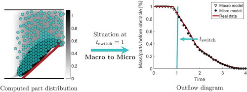
To validate the results of the switching procedure from micro to macro, the evolution of parts including the switch of the system is compared to real data, cf. (Göttlich et al., 2014). We measure how many mass or parts leave the system behind the obstacle, i.e. the outflow over time. The corresponding diagram is shown in Figure 4.

Figure 4. Switch from micro to macro for the material flow problem.

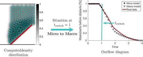
The maximal outflow error, meaning the maximal difference of the outflow of the model including the switch and the real data outflow, is about $6\mathrm{\%}$. The maximal outflow error of the macroscopic model without any switch is approximately $5\mathrm{\%}$ (see (Göttlich et al., 2014)), and thus indicates that the switch performs quite well.

The reverse situation, i.e. from macro to micro, is depicted in Figure 5. Here, the left picture shows the particle distribution resulting from the update algorithm 2. Even if the switch from the macroscopic to the microscopic representation is the more difficult direction, the maximal outflow error is now smaller compared to Figure 4. This is due to the higher accuracy of the microscopic model. The maximal outflow error, again compared to the real data outflow, is about $3.8\mathrm{\%}$.

Figure 5. Switch from macro to micro for the material flow problem.

5.2. Results for the pedestrian flow model

We consider an experimental setting with a room which has to be evacuated. Figure 6a shows the room geometry as well as the static velocity consisting of the desired velocity $v^0(x)$ and the wall forces $\sum _W{F}_W(x)$, see Figure 6b.

Figure 6. Evacuation of a room with one exit.

For the numerical implementation, almost the same parameters as in Helbing et al. (2000) are used. We choose the number of pedestrians as $N=81$, the mass $m=80$, the radius $r=0.25$, the desired velocity $\left|v^0\right|=1$, the acceleration time $\tau =0.5$, the constants $A=2000,B=0.08$ and the parameter $k=1.2\cdot {10}^5$. Since during the derivation, the tangential forces are neglected, we set $\kappa =0$ to directly compare the microscopic and macroscopic results. The final time horizon is $T=50$ and the time step to solve the Runge-Kutta scheme is $dt={10}^{-4}$.

The discretization of the force terms stated in Section 2.2 is straightforward, see (3.1) such that a classical Runge-Kutta method of fourth order is used again.

Corresponding to the discretization of the macroscopic Equation (3.4), the discretized version of the flux terms (3.3) is

$f^{(1)}(\rho ,{\rho }_{i,j}^k,{\mathit{x}}_{i+\frac{1}{2},j})=\sum _{p,q}{\rho }_{p,q}^k\cdot c_{i-p,j-q}^{(1)}$

with

$c_{p,q}^{(1)}={\int }_{Q_{p+\frac{1}{2},q}}Aexp\left(\frac{2r-\parallel {\mathit{x}}_{i+\frac{1}{2},j}-\mathit{y}\parallel }{B}\right)+k\cdot h(2r-\parallel {\mathit{x}}_{i+\frac{1}{2},j}-\mathit{y}\parallel )\frac{{\mathit{x}}_{i+\frac{1}{2},j}-\mathit{y}}{\parallel {\mathit{x}}_{i+\frac{1}{2},j}-\mathit{y}\parallel }d\mathit{y}$

and $Q_{p,q}=\left[x_{1,p-\frac{1}{2}},x_{1,p+\frac{1}{2}}\right]\times \left[x_{2,q-\frac{1}{2}},x_{2,q+\frac{1}{2}}\right]$ being a grid cell. The function $h$ is defined as before. For the external force term, it is

$g^{(1)}({\mathit{x}}_{i+\frac{1}{2},j})={\mathit{v}}^{0,(1)}({\mathit{x}}_{i+\frac{1}{2},j})+\frac{1}{m\lambda }\sum _W{F}_W^{(1)}({\mathit{x}}_{i+\frac{1}{2},j})$

with

${\mathit{F}}_W({\mathit{x}}_{i+\frac{1}{2},j})=\left(Aexp\left(\frac{r-d({\mathit{x}}_{i+\frac{1}{2},j})}{B}\right)+k\cdot h(r-d({\mathit{x}}_{i+\frac{1}{2},j}))\right){\mathit{n}}_W$

with $d({\mathit{x}}_{i+\frac{1}{2},j})$ the distance of point ${\mathit{x}}_{i+\frac{1}{2},j}$ to wall W.

We choose nearly the same parameters as in the microscopic case, i.e. only the parameters $A=1,B=0.1$ and $k=27$ have to be varied, to match the results of the pure microscopic simulation. As grid sizes, we have $\mathrm{\Delta }{x}_1=\mathrm{\Delta }{x}_2=0.1$ and $\mathrm{\Delta }t=0.001$.

Similar to the switch for the material flow model, a switch is implemented for the pedestrian model at time $t_{\mathrm{s}\mathrm{w}\mathrm{i}\mathrm{t}\mathrm{c}\mathrm{h}}=10.$ To compare the qualitative behavior of the models, the outflow at the door is measured. Since there is no real data available this time, the outflow of the model with switch is compared to the outflow without any switch, contrary to the material flow case.

Figure 7 shows the density distribution from the microscopic to macroscopic representation and the outflow behavior over time. As we can observe, the outflow of the switched model is close to the simulation results obtained from the microscopic simulation only. The maximal outflow error is about $5.3\mathrm{\%}$.

Figure 7. Switch from micro to macro for the pedestrian model.

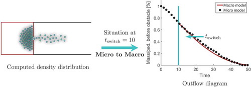
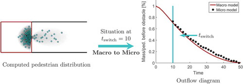
The results for the macro to micro switch can be found in Figure 8. Considering the outflow diagram, the results of the switched model are compared to the macroscopic simulation. The maximal outflow error is about $3.2\mathrm{\%}$, which is within an acceptable range.

Figure 8. Switch from macro to micro for the pedestrian model.

5.3. Computation times

Finally, we present the computation times for our switch implementation. All computations have been performed on a PC equipped with 16 GB Ram, Intel(R) Core(TM) i5-4690 [email protected] GHz. Tables 1 and 2 show the computation times for both switching directions (micro to macro and vice versa) and the two applications material and pedestrian flow. The same discretizations as introduced formerly are used. However, we remark that in the macro to micro direction the radius needs to be adapted in order to match the total mass (1.10).

Table 1. Computing times [sec] for the material flow model

$N$	Micro $\to$ Macro	Macro $\to$ Micro
		Start solution	Optimization	Update alg.	$\sum$
50	0.0077	0.19	25.84	0.17	26.21
100	0.0076	0.34	135.24	0.61	136.19
150	0.0075	0.48	274.08	1.48	276.05
200	0.0074	0.81	727.16	3.03	731.00

Table 2. Computing times [sec] for the pedestrian model

$N$	Micro $\to$ Macro	Macro $\to$ Micro
		Start solution	Optimization	Update alg.	$\sum$
50	0.0109	1.37	57.17	0.05	58.59
100	0.0098	1.10	919.42	0.03	920.56
150	0.0163	1.21	255.69	0.07	256.97
200	0.0153	1.34	2939.13	0.12	2940.60

The times for the three steps in the macro to micro direction are listed separately. As we can see, the most time-consuming part is the solution of the optimization problem (1.14) which takes several minutes up to almost one hour for $N=200$ objects, whereas the computation of the start solution (algorithm 1) as well as the update algorithm 2 takes only a couple of seconds.

The total computation time increases exponentially with the number of objects. Nevertheless, it might happen that an optimum is found quite fast, e.g. for $N=150$ pedestrians in Table 2. Note that the total computation times differ due to the different discretizations and geometries for the material and pedestrian flow models, cf. discussions in sub sections 4.1 and 4.2.

The computation time of the microscopic model (without any switch) increases quadratically in the number of objects $N$ (Göttlich et al., 2014). Therefore, the simulation of the macroscopic model provides a less costly alternative and good results. A switch to the microscopic representation is for instance useful if the user is interested in a better resolution of the underlying dynamics, even if the optimization step takes some time.

6. Conclusion

We have presented a switching method that allows to change dynamics from a microscopic to a macroscopic scale and vice versa. The method has been applied to material and pedestrian flow models to demonstrate the good numerical performance. In particular, the comparison of the material flow switch with real data shows quite promising results. Further research might include automatized switching decisions dewpending on suitable measures or discretizations (Agarwal & El-Sayed, 2018) as well as stochastic perturbations (Zhang et al., 2017).

Additional information

Funding

This work was supported by the German Research Foundation (DFG) under Grant OptiPlant [GO 1920/7-1] and by the Ministry of Science, Research and the Arts Baden-Württemberg and the University of Mannheim [Internal Open Access Publishing Fund].

Notes on contributors

Simone Göttlich

The Scientific Computing Research Group belongs to the Department of Mathematics at the University of Mannheim. It was founded in 2011 and directed since then by Prof. Göttlich. The research focuses on the mathematical modeling, numerical simulation and optimization of dynamic processes with applications in manufacturing systems, traffic flow and pedestrian dynamics and power grids.

References

- Agarwal, P., & El-Sayed, A. A. (2018). Non-standard finite difference and Chebyshev collocation methods for solving fractional diffusion equation. Physica A: Statistical Mechanics and Its Applications, 500, 40–49. doi:10.1016/j.physa.2018.02.014
- Aggarwal, A., Colombo, R. M., & Goatin, P. (2015). Nonlocal systems of conservation laws in several space dimensions. SIAM Journal Numerical Analysis, 53, 963–983. doi:10.1137/140975255
- Bellomo, N., Piccoli, B., & Tosin, A. (2012). Modeling crowd dynamics from a complex system viewpoint. Mathematical Models Methods Applications Sciences, 22, 1230004–1230029. doi:10.1142/S0218202512300049
- Carrillo, J. A., D’Orsogna, M. R., & Panferov, V. (2009). Double milling in self-propelled swarms from kinetic theory. Kinetic and Related Models, 2, 363–378. doi:10.3934/krm
- Cleary, P., & Sawley, M. (2002). DEM modelling of industrial granular flows: 3D case studies and the effect of particle shape on hopper discharge. Applied Mathematical Modelling, 26, 89–111. doi:10.1016/S0307-904X(01)00050-6
- Colombo, R. M., Garavello, M., & Lécureux-Mercier, M. (2012). A class of nonlocal models for pedestrian traffic. Mathematical Models Methods Applications Sciences, 22, 1150023. doi:10.1142/S0218202511500230
- Colombo, R. M., & Lécureux-Mercier, M. (2012). Nonlocal crowd dynamics models for several populations. Acta Mathematica Scientia, 32, 177–196. doi:10.1016/S0252-9602(12)60011-3
- Cristiani, E., Piccoli, B., & Tosin, A. (2011). Multiscale modeling of granular flows with application to crowd dynamics. Multiscale Modelling and Simulation, 9, 155–182. doi:10.1137/100797515
- Cristiani, E., Piccoli, B., & Tosin, A. (2014). Multiscale modeling of pedestrian dynamics, vol. 12 of MS&A. Modeling, Simulation and Applications. Cham: Springer.
- Cundall, P. A., & Strack, O. D. L. (1979). A discrete numerical model for granular assemblies. Géotechnique, 29, 47–65. doi:10.1680/geot.1979.29.1.47
- Degond, P., Ferreira, M. A., & Motsch, S. (2017). Damped Arrow-Hurwicz algorithm for sphere packing. Journal of Computational Physics, 332, 47–65. doi:10.1016/j.jcp.2016.11.047
- Etikyala, R., Göttlich, S., Klar, A., & Tiwari, S. (2014). Particle methods for pedestrian flow models: From microscopic to nonlocal continuum models. Mathematical Models Methods Applications Sciences, 24, 2503–2523. doi:10.1142/S0218202514500274
- Göttlich, S., Hoher, S., Schindler, P., Schleper, V., & Verl, A. (2014). Modeling, simulation and validation of material flow on conveyor belts. Applied Mathematical Modelling, 38, 3295–3313. doi:10.1016/j.apm.2013.11.039
- Göttlich, S., Klar, A., & Tiwari, S. (2015). Complex material flow problems: A multi-scale model hierarchy and particle methods. Journal of Engineering Mathematics, 92, 15–29. doi:10.1007/s10665-014-9767-5
- Göttlich, S., Knapp, S., & Schillen, P. (2017). A pedestrian flow model with stochastic velocities: Microscopic and macroscopic approaches. Retrieved from https://arxiv.org/pdf/1703.09134.pdf
- Helbing, D., Farkas, I., & Vicsek, T. (2000). Simulating dynamical features of escape panic. Nature, 407, 487–490.
- Herty, M., & Moutari, S. (2009). A macro-kinetic hybrid model for traffic flow on road networks. Computational Methods in Applied Mathematics, 9, 238–252. doi:10.2478/cmam-2009-0015
- Moutari, S., & Rascle, M. (2007). A hybrid Lagrangian model based on the Aw-Rascle traffic flow model. SIAM Journal Applications Mathematical, 68, 413–436. doi:10.1137/060678415
- Ruzhansky, M., Cho, Y., Agarwal, P., & Area, I. (2017). Advances in real and complex analysis with applications. Singapore: Trends in Mathematics, Springer.
- Zhang, X., Agarwal, P., Liu, Z., Peng, H., You, F., & Zhu, Y. (2017). Existence and uniqueness of solutions for stochastic differential equations of fractional-order q>1 with finite delays. Advances in Difference Equation, 2017, 123. 18.