The Gompertz Inverse Exponential (GoIE) distribution with applications

Abstract

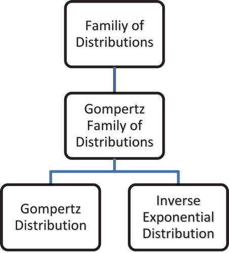
The Gompertz inverse exponential (GoIE) distribution using the Gompertz generalized family of distributions was derived and introduced in this article. Some basic statistical properties of the model were derived and discussed in minute details. The model parameters were estimated using the maximum likelihood estimation method. Real-life applications were provided and the GoIE distribution provides better fits than the Gompertz exponential, Gompertz Weibull and Gompertz Lomax distributions.

Keywords:

• generalized models
• Gompertz family of distributions
• inverse exponential
• mathematical statistics
• probability distributions

PUBLIC INTEREST STATEMENT

Extending existing probability distributions became necessary in recent years because of the need for models that can adequately fit or describe real-life events. The three-parameter probability model that was introduced in this article is however an extension of the one-parameter inverse exponential distribution. The extra two parameters are shape parameters due to the Gompertz family of distribution that was used. The role of these two extra parameters is to induce skewness into the inverse exponential distribution. As a consequence, the Gompertz inverse exponential distribution appears better than the Gompertz exponential, Gompertz Weibull and Gompertz Lomax distributions when applied to real-life datasets.

1. Introduction

The inverse exponential distribution is a special case of the inverse Weibull distribution; it has been introduced as far back as 1982 by Keller & Kamath (1982) and is capable of modelling datasets with inverted bathtub failure rate. It is a modification of the well-known exponential distribution and has an advantage of not having a constant failure rate. Because of this quality, it can be applied to describe real-life events in engineering, medicine and biology (especially, events with inverted bathtub failure rates). More details about the usefulness of the inverse exponential distribution have been discussed by Bakoban & Abu-Zinadah (2017), Lin, Duran, & Lewis (1989), Oguntunde & Adejumo (2015), Oguntunde, Babatunde, & Ogunmola (2014) and many others.

Recent studies in this line of research involve extending exiting probability distributions with the aim of increasing their modelling capability. Some attempts in the literature to increase the modelling capacity of the inverse exponential distribution include the works of Oguntunde, Adejumo, & Owoloko (2017a, 2017b, 2017c, 2017d) and Singh & Goel (2015); these works used different families of distributions to extend the inverse exponential distribution; a list of these families of distributions which include the beta generalized family of distribution (the first family of distribution developed from the logit of a random variable) and many others can be found in Alizadeh, Cordeiro, Bastos Pinho, & Ghosh (2017); Cordeiro, Alizadeh, Nascimeto, & Rasekhi (2016); Oguntunde, Adejumo, Okagbue, & Rastogi (2016); Oguntunde, Khaleel, Ahmed, Adejumo, & Odetunmibi (2017) and Owoloko, Oguntunde, & Adejumo (2015).

The interest of the article is, however, on the Gompertz family of distributions because it is relatively new and flexible. Unlike the beta generalized family of distribution, it does not include complex functions and thus is simpler to work with. It has been used in earlier works by Alizadeh et al. (2017) and Abdal-Hameed, Khaleel, Abdullah, Oguntunde, & Adejumo (2018), and its densities are as follows:

(1) $F\left(x\right)=1-e^{\frac{\alpha }{\beta }\left\{1-{\left[1-G\left(x\right)\right]}^{-\beta }\right\}};\alpha >0,\beta >0$(1)

and

(2) $f\left(x\right)=\alpha g\left(x\right){\left[1-G\left(x\right)\right]}^{-\beta -1}{e}^{\frac{\alpha }{\beta }\left\{1-{\left[1-G\left(x\right)\right]}^{-\beta }\right\}};\alpha >0,\beta >0$(2)

where $\alpha$ and $\beta$ are extra shape parameters and it was developed using the following transformation:

(3) $F\left(x\right)=\underset{0}{\overset{-log\left[1-G\left(x\right)\right]}{\int }}w\left(t\right)$(3)

$w\left(t\right)$ is the probability density function (pdf) of the Gompertz distribution and t is a random variable.

$G\left(x\right)$ and $g\left(x\right)$ are the cumulative distribution function (cdf) and pdf of the baseline distribution, respectively. In our case, the baseline distribution is the inverse exponential distribution defined as:

(4) $G\left(x\right)=e^{-\frac{\theta }{x}}$(4)

and

(5) $g\left(x\right)=\frac{\theta }{x^2}{e}^{-\frac{\theta }{x}}$(5)

where $\theta$ is regarded as the scale parameter.

2. The Gompertz inverse exponential distribution

The cdf of the Gompertz inverse exponential (GoIE) distribution is derived by substituting Equation (4) into Equation (1) to have:

(6) $F\left(x\right)=1-e^{\frac{\alpha }{\beta }\left\{1-{\left[1-e^{-\frac{\theta }{x}}\right]}^{-\beta }\right\}};\alpha >0,\beta >0,\theta >0$(6)

Also, the corresponding pdf is derived by substituting Equations (4) and (5) into Equation (2) to have:

(7) $f\left(x\right)=\alpha \frac{\theta }{x^2}{e}^{-\frac{\theta }{x}}{\left[1-e^{-\frac{\theta }{x}}\right]}^{-\beta -1}{e}^{\frac{\alpha }{\beta }\left\{1-{\left[1-e^{-\frac{\theta }{x}}\right]}^{-\beta }\right\}};\alpha >0,\beta >0,\theta >0$(7)

where $\alpha$ and $\beta$ are shape parameters and $\theta$ is the scale parameter

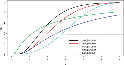
The pdf and cdf of the GoIE are represented in Figures 1 and 2, respectively, using different parameter values.

Figure 1. PDF of the GoIE distribution.

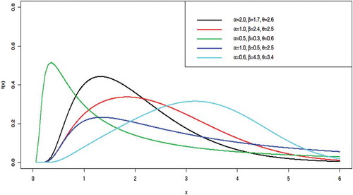
Figure 2. CDF of the GoIE distribution.

2.1. Some basic statistical properties of the Gompertz inverse exponential distribution

Some of the basic statistical properties of the GoIE are obtained as follows:

First, the reliability function is obtained by using the relation:

$S\left(x\right)=1-F\left(x\right)$

So, the reliability function of the GoIE distribution is:

(8) $S\left(x\right)=e^{\frac{\alpha }{\beta }\left\{1-{\left[1-e^{-\frac{\theta }{x}}\right]}^{-\beta }\right\}};\alpha >0,\beta >0,\theta >0$(8)

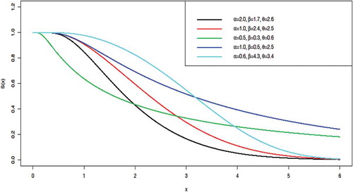
This is represented graphically in Figure 3.

Figure 3. Reliability function of GoIE distribution.

The failure rate of the GoIE distribution is obtained by dividing the pdf in Equation (7) by the reliability function in Equation (8) to have:

$h\left(x\right)=\frac{\alpha \frac{\theta }{x^2}{e}^{-\frac{\theta }{x}}{\left[1-e^{-\frac{\theta }{x}}\right]}^{-\beta -1}{e}^{\frac{\alpha }{\beta }\left\{1-{\left[1-e^{-\frac{\theta }{x}}\right]}^{-\beta }\right\}}}{e^{\frac{\alpha }{\beta }\left\{1-{\left[1-e^{-\frac{\theta }{x}}\right]}^{-\beta }\right\}}}$

(9) $h\left(x\right)=\alpha \frac{\theta }{x^2}{e}^{-\frac{\theta }{x}}{\left[1-e^{-\frac{\theta }{x}}\right]}^{-\beta -1};\alpha >0,\beta >0,\theta >0$(9)

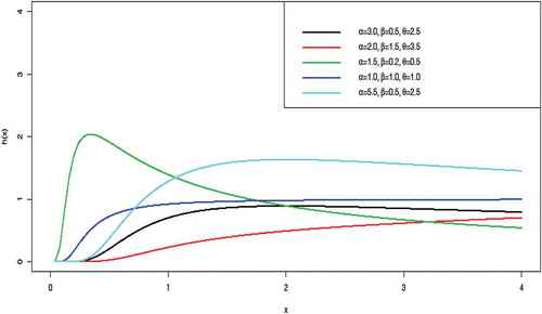
This is represented graphically in Figure 4.

Figure 4. Failure rate of the GoIE distribution.

The reversed hazard function of the GoIE distribution is obtained by dividing the pdf in Equation (7) by the cdf in Equation (6) to have:

(10) $r\left(x\right)=\frac{\alpha \frac{\theta }{x^2}{e}^{-\frac{\theta }{x}}{\left[1-e^{-\frac{\theta }{x}}\right]}^{-\beta -1}{e}^{\frac{\alpha }{\beta }\left\{1-{\left[1-e^{-\frac{\theta }{x}}\right]}^{-\beta }\right\}}}{1-e^{\frac{\alpha }{\beta }\left\{1-{\left[1-e^{-\frac{\theta }{x}}\right]}^{-\beta }\right\}}};\alpha >0,\beta >0,\theta >0$(10)

Also, the odds function is obtained by dividing the cdf in Equation (6) by the reliability function in Equation (8) to have:

(11) $O\left(x\right)=\frac{1-e^{\frac{\alpha }{\beta }\left\{1-{\left[1-e^{-\frac{\theta }{x}}\right]}^{-\beta }\right\}}}{e^{\frac{\alpha }{\beta }\left\{1-{\left[1-e^{-\frac{\theta }{x}}\right]}^{-\beta }\right\}}};\alpha >0,\beta >0,\theta >0$(11)

2.2. Quantile function and median

The quantile function $Q\left(u\right)$ is obtained from the relation:

$Q\left(u\right)=F^{-1}\left(u\right)$

So, the quantile function of the GoIE distribution is derived as:

(12) $Q\left(u\right)=-\theta ln{\left\{1-{\left[1-\frac{\beta ln\left(1-u\right)}{\alpha }\right]}^{-1/\beta }\right\}}^{-1}$(12)

where $u-Uniform\left(0,1\right)$. In other words, random samples from the GoIE distribution can be generated using:

$x=-\theta ln{\left\{1-{\left[1-\frac{\beta ln\left(1-u\right)}{\alpha }\right]}^{-1/\beta }\right\}}^{-1}$

The median of the GoIE distribution can conveniently be derived by making the substitution of $u=0.5$ in Equation (12) to have:

(13) $Median=-\theta ln{\left\{1-{\left[1-\frac{\beta ln\left(0.5\right)}{\alpha }\right]}^{-1/\beta }\right\}}^{-1}$(13)

The corresponding first quartile and third quartile can also be obtained by making the substitution of $u=0.25$ and $u=0.75$, respectively, into Equation (12).

2.3. Order statistics

The pdf of the $jth$ order statistic for a random sample of size $n$ from a distribution function $F\left(x\right)$ and an associated pdf $f\left(x\right)$ is given by:

(14) $f_{j:n}\left(x\right)=\frac{n!}{\left(j-1\right)!\left(n-j\right)!}f\left(x\right){\left[F\left(x\right)\right]}^{j-1}{\left[1-F\left(x\right)\right]}^{n-j}$(14)

where $f\left(x\right)$ and $F\left(x\right)$ are the pdf and cdf of the GoIE, respectively. The pdf of the jth order statistics for a random sample of size $n$ from the GoIE distribution is, however, given as follows:

(15) $f_{j:n}\left(x\right)=\frac{n!}{\left(j-1\right)!\left(n-j\right)!}\left\{\alpha \frac{\theta }{x^2}{e}^{-\frac{\theta }{x}}{\left[1-e^{-\frac{\theta }{x}}\right]}^{-\beta -1}{e}^{\frac{\alpha }{\beta }\left\{1-{\left[1-e^{-\frac{\theta }{x}}\right]}^{-\beta }\right\}}\right\}{\left[1-e^{\frac{\alpha }{\beta }\left\{1-{\left[1-e^{-\frac{\theta }{x}}\right]}^{-\beta }\right\}}\right]}^{j-1}{\left[e^{\frac{\alpha }{\beta }\left\{1-{\left[1-e^{-\frac{\theta }{x}}\right]}^{-\beta }\right\}}\right]}^{n-j}$(15)

So, the pdf of minimum order statistics is obtained by substituting $j=1$ in Equation (15) to have:

(16) $f_{1:n}\left(x\right)=n\left\{\alpha \frac{\theta }{x^2}{e}^{-\frac{\theta }{x}}{\left[1-e^{-\frac{\theta }{x}}\right]}^{-\beta -1}{e}^{\frac{\alpha }{\beta }\left\{1-{\left[1-e^{-\frac{\theta }{x}}\right]}^{-\beta }\right\}}\right\}{\left[e^{\frac{\alpha }{\beta }\left\{1-{\left[1-e^{-\frac{\theta }{x}}\right]}^{-\beta }\right\}}\right]}^{n-1}$(16)

While the corresponding pdf of maximum order statistics is obtained by making the substitution of $j=n$ in Equation (15) as:

(17) $f_{n:n}\left(x\right)=n\left\{\alpha \frac{\theta }{x^2}{e}^{-\frac{\theta }{x}}{\left[1-e^{-\frac{\theta }{x}}\right]}^{-\beta -1}{e}^{\frac{\alpha }{\beta }\left\{1-{\left[1-e^{-\frac{\theta }{x}}\right]}^{-\beta }\right\}}\right\}{\left[1-e^{\frac{\alpha }{\beta }\left\{1-{\left[1-e^{-\frac{\theta }{x}}\right]}^{-\beta }\right\}}\right]}^{n-1}$(17)

2.4. Estimation

The method of maximum likelihood estimation is used to estimate the parameters of the GoIE distribution. For a random sample $x_1,x_2,...,x_n$ distributed according to the cdf of the GoIE distribution, the log-likelihood function is obtained as:

(18) $f\left(x_1,x_2,...,x_n;\alpha ,\beta ,\theta \right)=\prod _{i=1}^n\left[\alpha \frac{\theta }{x_i^2}{e}^{-\frac{\theta }{x_i}}{\left[1-e^{-\frac{\theta }{x_i}}\right]}^{-\beta -1}{e}^{\frac{\alpha }{\beta }\left\{1-{\left[1-e^{-\frac{\theta }{x_i}}\right]}^{-\beta }\right\}}\right]$(18)

The log-likelihood function $L$ is obtained as:

(19) $L=nln\left(\alpha \right)+nln\left(\theta \right)-2\sum _{i=1}^{n}ln\left(x_i\right)-\sum _{i=1}^n\left(\frac{\theta }{x_i}\right)-\left(\beta +1\right)\sum _{i=1}^{n}ln\left[1-e^{-\frac{\theta }{x_i}}\right]+\frac{\alpha }{\beta }\sum _{i=1}^n\left\{1-{\left[1-e^{-\frac{\theta }{x_i}}\right]}^{-\beta }\right\}$(19)

Differentiate $L$ with respect to parameters $\alpha ,\beta$ and $\theta$ and equate the results to zero, and solving the resulting simultaneous equations gives the parameter estimates. The solution may not be obtained in closed form; so, software can be used to obtain the estimates numerically; example of such software include R, MAPLE and so on.

3. Model validation and application

The GoIE distribution is applied to two datasets and comparisons are made with the Gompertz exponential, Gompertz Weibull and Gompertz Lomax distributions. R software was used for the analysis and the criteria used for model selection are Akaike information criteria (AIC), consistent Akaike information criteria (CAIC), Bayesian information criteria (BIC), negative log-likelihood (NLL) and Hannan and Quinn information criteria (HQIC).

The criteria for selecting the distribution with the best fit depends on the values of the AIC, CAIC, BIC, NLL and HQIC, and lower values of this criteria indicate a better fit.

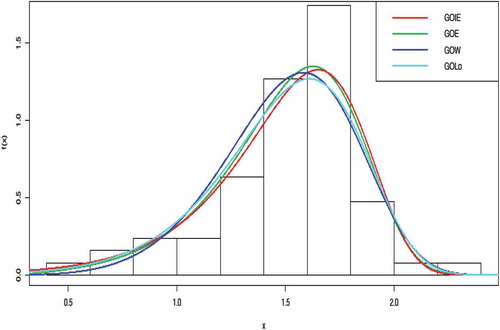
First Illustration: A data relating to the strengths of 1.5cm glass fibres which has been analysed previously by Oguntunde et al. (2017) and Bourguignon, Silva, & Cordeiro (2014), Merovci, Khaleel, Ibrahim, & Shitan (2016) Smith & Naylor (1987) was used. The observations are:

0.55, 0.74, 0.77, 0.81, 0.84, 1.24, 0.93, 1.04, 1.11, 1.13, 1.30, 1.25, 1.27, 1.28, 1.29, 1.48, 1.36, 1.39, 1.42, 1.48, 1.51, 1.49, 1.49, 1.50, 1.50, 1.55, 1.52, 1.53, 1.54, 1.55, 1.61, 1.58, 1.59, 1.60, 1.61, 1.63, 1.61, 1.61, 1.62, 1.62, 1.67, 1.64, 1.66, 1.66, 1.66, 1.70, 1.68, 1.68, 1.69, 1.70, 1.78, 1.73, 1.76, 1.76, 1.77, 1.89, 1.81, 1.82, 1.84, 1.84, 2.00, 2.01, 2.24

The result of the analysis is displayed in Table 1.

Table 1. Table of result

Models	Estimates	NLL	AIC	CAIC	BIC	HQIC	Rank
GoIE (Proposed)	$\begin{array}{c}\stackrel{\wedge }{\alpha }=0.2030548\\ \stackrel{\wedge }{\beta }=11.5541435\\ \stackrel{\wedge }{\theta }=2.0003185\end{array}$	14.04093	34.08187	34.48865	40.51127	36.61059	1
GoExp (New)	$\begin{array}{c}\stackrel{\wedge }{\alpha }=-0.004768848\\ \stackrel{\wedge }{\beta }=-1.810999364\\ \stackrel{\wedge }{\theta }=-1.987714978\end{array}$	14.81765	35.6353	36.04208	42.06471	38.16402	2
GoWei (New)	$\begin{array}{c}\stackrel{\wedge }{\alpha }=0.228488761\\ \stackrel{\wedge }{\beta }=0.009628097\\ \stackrel{\wedge }{\theta }=0.794918813\\ \stackrel{\wedge }{\lambda }=5.612111282\end{array}$	15.18847	38.37694	39.06659	46.94948	41.74856	4
GoLom (Developed by Oguntunde et al. [2017])	$\begin{array}{c}\stackrel{\wedge }{\alpha }=0.004592168\\ \stackrel{\wedge }{\beta }=8.179090955\\ \stackrel{\wedge }{\theta }=0.506999370\\ \stackrel{\wedge }{\lambda }=1.515829085\end{array}$	14.50274	37.00548	37.69513	45.57802	40.3771	3

The GoIE is adjudged the distribution with the best fit because it has the lowest AIC, CAIC, BIC, NLL and HQIC values.

The histogram of the data with the competing distributions is displayed in Figure 5.

Figure 5. Histogram of the first data with the competing distributions.

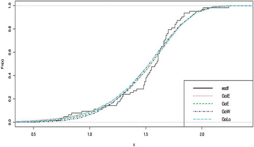
The empirical cdf of the competing distributions with respect to the dataset used is displayed in Figure 6.

Figure 6. The empirical cdf of the first data together with the competing distributions.

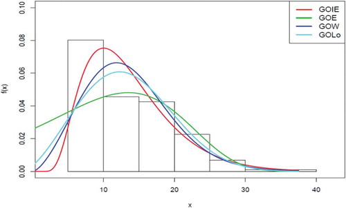
Second Illustration: A sport data which is downloadable at www.stat.auckland.ac.nz/~lee/330/datasets.dir/sport.data was used and the observations are:

19.75, 21.30, 19.88, 23.66, 17.64, 15.58, 19.99, 22.43, 17.95, 15.07, 28.83, 18.08, 23.30, 17.71, 18.77, 19.83, 25.16, 18.04, 21.79, 22.25, 16.25, 16.38, 19.35, 19.20, 17.89, 12.20, 23.70, 24.69, 16.58, 21.47, 20.12, 17.51, 23.70, 22.39, 20.43, 11.29, 25.26, 19.39, 19.63, 23.11, 16.86, 21.32, 26.57, 17.93, 24.97, 22.62, 15.01, 18.14, 26.78, 17.22, 26.50, 23.01, 30.10, 13.93, 26.65, 35.52, 15.59, 19.61, 14.52, 11.47, 17.71, 18.48, 11.22, 13.61, 12.78, 11.85, 13.35, 11.77, 11.07, 21.30, 20.10, 24.88, 19.26, 19.51, 23.01, 8.07, 11.05, 12.39, 15.95, 9.91, 16.20, 9.02, 14.26, 10.48, 11.64, 12.16, 10.53, 10.15, 10.74, 20.86, 19.64, 17.07, 15.31, 11.07, 12.92, 8.45, 10.16, 12.55, 9.10, 13.46, 8.47, 7.68, 6.16, 8.56, 6.86, 9.40, 9.17, 8.54, 9.20, 11.72, 8.44, 7.19, 6.46, 9.00, 12.61, 9.03, 6.96, 10.05, 9.56, 9.36, 10.81, 8.61, 9.53, 7.42, 9.79, 8.97, 7.49, 11.95, 7.35, 7.16, 8.77, 9.56, 14.53, 8.51, 10.64, 7.06, 8.87, 7.88, 9.20, 7.19, 6.06, 5.63, 6.59, 9.50, 13.97, 11.66, 6.43, 6.99, 6.00, 6.56, 6.03, 6.33, 6.82, 6.20, 5.93, 5.80, 6.56, 6.76, 7.22, 8.51, 7.72, 19.94, 13.91, 6.10, 7.52, 9.56, 6.06, 7.35, 6.00, 6.92, 6.33, 5.90, 8.84, 8.94, 6.53, 9.40, 8.18, 17.41, 18.08, 9.86, 7.29, 18.72, 10.12, 19.17, 17.24, 9.89, 13.06, 8.84, 8.87, 14.69, 8.64, 14.98, 7.82, 8.97, 11.63, 13.49, 10.25, 11.79, 10.05, 8.51, 11.50, 6.26

The result of the analysis is displayed in Table 2.

Table 2. Table of result

Models	Estimates	NLL	AIC	CAIC	BIC	HQIC	Rank
GoIE (Proposed)	$\begin{array}{c}\stackrel{\wedge }{\alpha }=4.636970\\ \stackrel{\wedge }{\beta }=1.583631\\ \stackrel{\wedge }{\theta }=25.794220\end{array}$	629.335	1264.67	1234.791	1274.595	1268.686	1
GoExp (New)	$\begin{array}{c}\stackrel{\wedge }{\alpha }=5.330925317\\ \stackrel{\wedge }{\beta }=20.978768343\\ \stackrel{\wedge }{\theta }=0.004836174\end{array}$	663.8036	1333.607	1333.728	1343.532	1337.623	4
GoWei (New)	$\begin{array}{c}\stackrel{\wedge }{\alpha }=11.22264866\\ \stackrel{\wedge }{\beta }=-1.29977338\\ \stackrel{\wedge }{\theta }=0.02630932\\ \stackrel{\wedge }{\lambda }=2.54531004\end{array}$	641.4217	1290.843	1291.046	1304.076	1296.197	2
GoLom (Developed by Oguntunde et al. [2017])	$\begin{array}{c}\stackrel{\wedge }{\alpha }=0.006519876\\ \stackrel{\wedge }{\beta }=3.370057658\\ \stackrel{\wedge }{\theta }=0.714843759\\ \stackrel{\wedge }{\lambda }=0.747124582\end{array}$	645.6623	1299.325	1299.528	1312.558	1304.679	3

The GoIE is also adjudged the distribution with the best fit because it has the lowest AIC, CAIC, BIC, NLL and HQIC values.

The histogram of the second data with the competing distributions is displayed in Figure 7.

Figure 7. Histogram of the second data with the competing distributions.

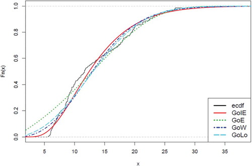
The empirical cdf of the competing distributions with respect to the second dataset is displayed in Figure 8.

Figure 8. The empirical cdf of the second data together with the competing distributions.

4. Discussion

The results from Tables 1 and 2 show that the GoIE has the lowest values for all the criteria used. So, the GoIE distribution is considered the best model to fit the datasets among the other distributions used. This is also evident in the plots provided in Figure 5–8. In Figures 5 and 7, the red curve which represents GoIE distribution has the highest peak compared to others. Also in Figures 6 and 8, the red line is closer to the empirical cdf of the datasets than others.

5. Conclusion

The GoIE distribution has been successfully introduced in this paper and some of its basic statistical properties have been obtained. The pdf of the model and its failure rate have unimodal shapes; this means that the model would be useful to fit real-life events with unimodal failure rates. The model is tractable and flexible and shows high modelling capability as it performs better than the Gompertz exponential, Gompertz Weibull and Gompertz Lomax distributions; this was judged based on the AIC, CAIC, BIC, NLL and HQIC values of these distributions. The GoIE distribution is of no doubt a competitive model, and it is hoped that it would be of use in fields like engineering, biology and medicine. Some other statistical properties of the distribution (which were not considered in this paper) can be explored and simulation study can also be conducted.

Acknowledgements

The authors appreciate Covenant University for providing an enabling environment for this research. The efforts of the reviewers are greatly appreciated.

Additional information

Funding

The authors received no direct funding for this research.

Notes on contributors

Pelumi E. Oguntunde

Dr. Pelumi E. Oguntunde is a Statistician and a faculty in the Department of Mathematics, Covenant University, Nigeria. He has Bachelor of Science (B.Sc.) and Master of Science (M.Sc.) degrees in Statistics from University of Ilorin and University of Ibadan respectively. He earned his Ph.D. degree in Industrial Mathematics (Statistics Option) from Covenant University, Nigeria. His area of specialization is Mathematical Statistics. He teaches Statistics courses and he has made noticeable contributions to several scholarly journals especially in the area of probability distributions.

References

- Abdal-Hameed, M., Khaleel, M. A., Abdullah, Z. M., Oguntunde, P. E., & Adejumo, A. O. (2018). Parameter estimation and reliability, hazard functions of Gompertz Burr Type XII distribution. Tikrit Journal for Administration and Economics Sciences, 1(41 part 2), 381–400.
- Alizadeh, M., Cordeiro, G. M., Bastos Pinho, L. G., & Ghosh, I. (2017). The Gompertz-g family of distributions. Journal of Statistical Theory and Practice, 11(1), 179–207. doi:10.1080/15598608.2016.1267668
- Bakoban, R. A., & Abu-Zinadah, H. H. (2017). The beta generalized inverted exponential distribution with real data applications. REVSTAT-Statistical Journal, 15(1), 65–88.
- Bourguignon, M., Silva, R. B., & Cordeiro, G. M. (2014). The Weibull-G family of probability distributions. Journal of Data Science, 12, 53–68.
- Cordeiro, G. M., Alizadeh, M., Nascimeto, A. D. C., & Rasekhi, M. (2016). The exponentiated Gompertz generated family of distributions: Properties and applications. Chilean Journal of Statistics, 7(2), 29–50.
- Keller, A. Z., & Kamath, A. R. (1982). Reliability analysis of CNC machine tools. Reliability Engineering, 3, 449–473. doi:10.1016/0143-8174(82)90036-1
- Lin, C. T., Duran, B. S., & Lewis, T. O. (1989). Inverted gamma as life distribution. Microelectron Reliability, 29(4), 619–626. doi:10.1016/0026-2714(89)90352-1
- Merovci, F., Khaleel, M. A., Ibrahim, N. A., & Shitan, M. (2016). The beta type X distribution: Properties with applications. SpringerPlus, 5, 697. doi:10.1186/s40064-016-2271-9
- Oguntunde, P. E., & Adejumo, A. O. (2015). The transmuted inverse exponential distribution. International Journal of Advanced Statistics and Probability, 3(1), 1–7. doi:10.14419/ijasp.v3i1.3684
- Oguntunde, P. E., Adejumo, A. O., Okagbue, H. I., & Rastogi, M. K. (2016). Statistical properties and applications of a new Lindley exponential distribution. Gazi University Journal of Science, 29(4), 831–838.
- Oguntunde, P. E., Adejumo, A. O., & Owoloko, E. A. (2017a). Application of Kumaraswamy inverse exponential distribution to real lifetime data. International Journal of Applied Mathematics and Statistics, 56(5), 34–47.
- Oguntunde, P. E., Adejumo, A. O., & Owoloko, E. A. (2017b, July 5–7). On the flexibility of the transmuted inverse exponential distribution. Lecture Notes on engineering and computer science: Proceeding of the World Congress on Engineering (pp. 123–126). London, UK.
- Oguntunde, P. E., Adejumo, A. O., & Owoloko, E. A. (2017c, July 5–7). On the exponentiated generalized inverse exponential distribution. Lecture Notes on engineering and computer science: Proceeding of the World Congress on Engineering (pp. 80–83). London, UK.
- Oguntunde, P. E., Adejumo, A. O., & Owoloko, E. A. (2017d, July 5–7). The Weibull-inverted exponential distribution: A generalization of the inverse exponential distribution. Lecture Notes on engineering and computer science: Proceeding of the World Congress on Engineering (pp. 16–19). London, UK.
- Oguntunde, P. E., Babatunde, O. S., & Ogunmola, A. O. (2014). Theoretical analysis of the Kumaraswamy-inverse exponential distribution. International Journal of Statistics and Applications, 4(2), 113–116.
- Oguntunde, P. E., Khaleel, M. A., Ahmed, M. T., Adejumo, A. O., & Odetunmibi, O. A. 2017. A new generalization of the Lomax distribution with increasing, decreasing and constant failure rate. Article ID 6043169 Modelling and Simulation in Engineering, 2017, 6. doi:10.1155/2017/6043169
- Owoloko, E. A., Oguntunde, P. E., & Adejumo, A. O. (2015). Performance rating of the transmuted exponential distribution. An Analytical Approach, SpringerPlus, 4, 818.
- Singh, B., & Goel, R. (2015). The beta inverted exponential distribution: Properties and applications. International Journal of Applied Sciences and Mathematics, 2(5), 132–141.
- Smith, R. I., & Naylor, J. C. (1987). A comparison of maximum likelihood and Bayesian estimators for the three-parameter Weibull distribution. Applied Statistics, 36, 258–369. doi:10.2307/2347795