Efficient estimation of distributed lag model in presence of heteroscedasticity of unknown form: A Monte Carlo evidence

Abstract

In the presence of heteroscedasticity, the ordinary least-squares (OLS) estimator remains no more efficient while the popular Almon technique is being considered for a finite distributed lag model (DLM). The available literature proposes few adaptive estimators which are more efficient than the OLS estimator when there is heteroscedasticity of unknown form. This study suggests the similar adaptation combined with the Almon technique in order to get more efficient estimator of vector of lag coefficients in the DLM. Performance of the proposed estimator has been evaluated through the Monte Carlo simulations. The simulation results show an attractive performance of the proposed estimator in terms of efficiency.

Keywords:

• adaptive estimator
• Almon technique
• finite distributed lag model
• heteroscedasticity

AMS Subject Classification:

• 62J05
• 62J99

PUBLIC INTEREST STATEMENT

A distributed lag model (DLM) is a model for a sort of time series data in which a regression equation is used to predict current values of a dependent variable based on both the current values of an explanatory variable and the past period (lagged) values of this explanatory variable. Precisely, a DLM is a dynamic model in which the effect of a regressor on regressand occurs over time rather than all at once. The non-constant variances of the error term (i.e., issue of heteroscedasticity), associated with such model, may result in inefficient estimation of the unknown coefficients of the stated DLM. This paper addresses the same issue and suggests some more efficient estimation method.

1. Introduction

The distributed lag model (DLM) includes lagged values of independent variables as explanatory variables. The use of such model is motivated by the fact that the effect of change in an independent variable is not always completely exhausted within one time period but is “distributed” over several, and perhaps many, future periods. The DLM has gained paramount importance because of its frequent use in econometrics and statistics. However, estimation of the DLM has remained core issue for many researchers because of two problems that are almost certain to arise when the ordinary least-squares (OLS) method is applied directly to this model. Firstly, if the number of lags is large enough but the sample size is small, it may not be possible to infer about the parameters because of inadequate degrees of freedom to carry out the traditional tests of significance. Secondly, in most of the economic time series, the successive (lag) values tend to be highly correlated causing the problem of multicollinearity which leads to imprecise estimation of parameters because the variances of estimates tend to be large due to multicollinearity among explanatory variables (Baltagi, 2011; Gujarati, 2003; Maddala, 1977). To overcome these problems, various methods have been proposed by different researchers (Almon, 1965; Koyck, 1954; Shiller, 1973) for estimation of the DLM. All these methods are based on some prior knowledge about the behaviour of parameters and this source of prior knowledge includes non-stochastic and stochastic smoothness priors (Gujarati, 2003; Vinod & Ullah, 1981). Among the available methods proposed for estimation of the DLM, a technique of polynomial distributed lag (PDL) proposed by Almon (1965) has gained much popularity. In Almon’s technique, the DLM is transformed into a model which has fewer explanatory variables and thus, severity of collinearity reduces considerably. This technique not only reduces the effect of multicollinearity but it also reduces the number of parameters to be estimated in the DLM (Maddala, 1977). The Almon procedure is based on the assumption that parameters in the DLM lie on some polynomial of suitable degree.

Application of the OLS, combined with the Almon technique, requires that the DLM meets all the assumptions about the error term which are considered for a classical linear regression model. The assumption of homoscedasticity is considered as one of the important assumptions which states that the error variances are constant across all the observations. But in practice, this assumption is frequently violated and the random errors in such case are said to be heteroscedastic. In the presence of heteroscedasticity, the usual OLS estimator (OLSE) remains unbiased, consistent and asymptotically normal but becomes inefficient and its usual covariance matrix estimator becomes biased and inconsistent.

If the form of heteroscedasticity is known, the method of weighted least-squares (WLS) is the best choice to get efficient estimates of parameters but the form of heteroscedasticity is seldom known. In such situation, the estimated weighted least-squares (EWLS) estimator can be used which can provide more efficient estimates than the OLSE (Fuller & Rao, 1978; Pasha, 1982). Besides this, some adaptive estimators have been proposed which are more efficient than the OLSE (Carroll, 1982; Carroll & Ruppert, 1982; Robinson, 1987). A vast literature (Ahmed, Aslam, & Pasha, 2011; Aslam, 2006, 2014; Aslam, Riaz, & Altaf, 2013) is available to justify the use of such adaptive estimators as a substitute of the OLSE in the presence of heteroscedasticity of unknown form. However, estimation of DLM by the Almon technique in presence of heteroscedastic errors has not grabbed the attention of researchers. This paper addresses this issue and proposes the use of adaptive estimator combined with the Almon technique as a replacement of the OLSE for efficient estimation of the DLM in the presence of heteroscedasticity of unknown form.

This paper is organized as follows. Section 2 describes the DLM with heteroscedastic errors and the adaptive estimation. Section 3 briefly describes the Monte Carlo scheme and data generating process along with the results. Section 4 concludes the paper.

2. The distributed lag model and adaptive estimation

The general form of a finite DLM is

(1) $y_t={\beta }_0{x}_t+{\beta }_1{x}_{t-1}+\dots +{\beta }_s{x}_{t-s}+u_t,t=s+1,\dots ,T$(1)

$=\sum _{i=0}^s{\beta }_i{x}_{t-i}+u_t.$

In matrix notation, the model in Equation (1) can be written as follows:

(2) $y=X\beta +u,$(2)

where

$y=\left[\begin{array}{c}{y}_{s+1}\\ \begin{array}{c}{y}_{s+2}\\ \begin{array}{c}⋮\\ y_T\end{array}\end{array}\end{array}\right],\beta =\left[\begin{array}{c}{\beta }_0\\ \begin{array}{c}{\beta }_1\\ \begin{array}{c}⋮\\ {\beta }_s\end{array}\end{array}\end{array}\right],X=\left[\begin{array}{cccc}{x}_{s+1}& x_s& \dots & x_1\\ x_{s+2}& x_{s+1}& \dots & x_2\\ ⋮& ⋮& ⋮& ⋮\\ x_T& x_{T-1}& \dots & x_{T-s}\end{array}\right],u=\left[\begin{array}{c}{u}_{s+1}\\ \begin{array}{c}{u}_{s+2}\\ \begin{array}{c}⋮\\ u_T\end{array}\end{array}\end{array}\right].$

Clearly, $\mathrm{y}$ is a $\left(T-s\right)\times 1$ vector of observations on response variable,$\beta$ is a $\left(s+1\right)\times 1$ vector of unknown lag coefficients or lag weights, $u$ is a vector of random error with mean zero and variance $\mathrm{\Omega }$ with tth diagonal elements ${\sigma }_t^2$ i.e., $\mathrm{\Omega }=diag\left\{{\sigma }_{s+1}^2,{\sigma }_{s+2}^2,\dots ,{\sigma }_T^2\right\}$. When the error term is homoscedastic, ${\sigma }_t^2={\sigma }^2$ and $\mathrm{\Omega }={\sigma }^2{I}_{\left(T-s\right)}$, where I_(T-s) is an identity matrix of order $\left(T-s\right)$.

Direct application of the OLS to estimate DLM given in Equation (1) may have some serious problems as discussed earlier. For estimation of the DLM, Almon (1965) proposed a technique which is widely used by the practitioners. Almon assumed that the coefficients ${\beta }_i$ could be well approximated by a polynomial of degree r in i which was less than s (the lag length) i.e.,

(3) ${\beta }_i={\alpha }_0+{\alpha }_{1}i+{\alpha }_2{i}^2+\dots +{\alpha }_r{i}^r;i=0,1,2,\dots ,sands\ge r\ge 0$(3)

Substituting Equation (3) in Equation (1), one can estimate $\alpha$ by the usual OLS procedure and then using Equation (3), one can get the estimates of ${\beta }_i$. In matrix notations, Equation (3) can be written as

(4) $\beta =A\alpha ,$(4)

where $\beta$ is as mentioned before and

$A=\left[\begin{array}{ccccc}1& 0& 0& \cdots & 0\\ 1& 1& 1& \cdots & 1\\ ⋮& ⋮& ⋮& ⋮& ⋮\\ 1& s& s^2& \cdots & s^r\end{array}\right],\alpha =\left[\begin{array}{c}{\alpha }_0\\ {\alpha }_1\\ ⋮\\ {\alpha }_r\end{array}\right]$

are $\left(s+1\right)\times \left(r+1\right)$ matrix and $\left(r+1\right)\times 1$ vector, respectively. By substituting Equation (4) in Equation (2), one can obtain

(5) $\begin{array}{rl}& y=XA\alpha +u,\\ & =Za+u.\end{array}$(5)

Here, $Z=XA$ The OLS estimator of $\alpha$ is as follows:

${\hat{\alpha }}_{OLS}={\left(Z^{\prime }Z\right)}^{-1}{Z}^{\prime }y={\left(A^{\prime }{X}^{\prime }XA\right)}^{-1}{A}^{\prime }{X}^{\prime }y,$

The parameter vector β can be estimated as follows:

$\hat{\beta }=A\hat{\alpha },$

which is the Almon estimator of $\beta$. If the error term is homoscedastic, it is the best linear unbiased estimator (BLUE) of $\beta$ (Judge, Griffiths, Hill, Lütkepohl, & Lee, 1980). A major advantage of the Almon technique is that if a distributed lag is assumed to lie on a polynomial of a specified degree then the distributed lag can be estimated by standard linear regression methods (Fair & Jaffee, 1971). Moreover, the Almon technique reduces the effect of multicollinearity (Fair & Jaffee, 1971; Judge et al., 1980; Maddala, 1977) because there are fewer explanatory variables in the transformed model as compared to the actual DLM.

In the presence of heteroscedasticity, ${\hat{\alpha }}_{OLS}$ does not remain efficient and consequently $\hat{\beta }$ also becomes inefficient. Thus, some efficient estimator of $\alpha$ is desired which will further give an efficient estimator of $\beta$. The WLS estimator is one possible solution to estimate model (5) efficiently if ${\sigma }_t^2$ are known. Let $W=diag\left\{w_{s+1},w_{s+2},\dots ,w_T\right\}$ be the diagonal matrix of weights whose tth diagonal element $w_t={\sigma }_t^{-2}$ then the WLS estimator is

${\hat{\alpha }}_{WLS}={\left(Z^{\prime }\hat{W}Z\right)}^{-1}{Z}^{\prime }\hat{W}y.$

However, in practical situations, ${\sigma }_t^2$ are usually not known and their estimates are used. The resulting EWLS estimator of the parametric vector $\alpha$ is

${\hat{\alpha }}_{EWLS}={\left(Z^{\prime }\hat{W}Z\right)}^{-1}{Z}^{\prime }\hat{W}y,$

where $\hat{W}$ is a nonsingular diagonal matrix containing estimated weights used for variance-stabilizing transformation.

Now the concern is to construct $\hat{W}$ and for this purpose, an adaptive estimator proposed by Carroll (1982) can be used. Carroll (1982) assumed the error variance to be a smooth function of the mean values as:

${\sigma }_t^2=g\left({\tau }_t\right),$

where $g$ is unknown and ${\tau }_t=Z_t^{\mathrm{\prime }}\alpha .$ The estimate of${\tau }_t$, in context of model (5), is given as follows:

${\hat{\tau }}_t=Z_t^{\mathrm{\prime }}{\hat{\alpha }}_{OLS.}$

Carroll (1982) presented the kernel estimator of ${\sigma }_t^2$ in the form of Nadaraya-Watson (Nadaraya, 1964; Watson, 1964) estimator as

${\hat{\sigma }}_t^2=\frac{{\sum }_{j=s+1}^{T}K\left(\frac{{\hat{\tau }}_j-{\hat{\tau }}_t}{h}\right){\hat{u}}_j^2}{{\sum }_{j=s+1}^{T}K\left(\frac{{\hat{\tau }}_j-{\hat{\tau }}_t}{h}\right)},$

where $K\left(\cdot \right)$ is the kernel function with smoothing parameter $h$ and ${\hat{u}}_j$ are the OLS residuals of model (5).

Thus we have ${\hat{W}}_A=diag\left\{{\hat{w}}_{s+1},{\hat{w}}_{s+2},\dots ,{\hat{w}}_T\right\}$, where ${\hat{w}}_t={\hat{\sigma }}_t^{-2}$ and the adaptive weighted least-squares (AWLS) estimator of $\alpha$can be defined as follows:

${\hat{\alpha }}_{AWLS}={\left(Z^{\prime }{\hat{W}}_{A}Z\right)}^{-1}{Z}^{\prime }{\hat{W}}_{A}y.$

Carroll (1982) proved that ${\hat{\alpha }}_{AWLS}$ has the same asymptotic properties as that of the WLS estimator (i.e., ${\hat{\alpha }}_{WLS}$), based on the true weights. It has a normal limiting distribution with mean $\alpha$ and covariance ${\left(Z^{\prime }WZ\right)}^{-1}$. Furthermore, such adaptive estimator is more efficient than the OLSE in the presence of heteroscedasticity of unknown form (for more details, see Carroll [10, p. 1226–1227]).

The use of such efficient estimator combined with the Almon technique may increase the efficiency of the Almon estimator when a DLM is plagued with the heteroscedasticity of unknown form. Therefore, an efficient estimator of parameter vector $\beta$ based on adaptive estimator ${\hat{\alpha }}_{\mathrm{A}\mathrm{W}\mathrm{L}\mathrm{S}}$ can be given as follows:

${\hat{\beta }}_{AWLS}=A{\hat{\alpha }}_{AWLS}.$

3. Numerical evaluation

Following Frost (1975) and Güler, Gültay, and Kaçiranlar (2017), we used the following model to generate observations:

(6) $y_t={\beta }_0{x}_t+{\beta }_1{x}_{t-1}+\dots +{\beta }_s{x}_{t-s}+u_t,$(6)

(7.a) $x_1=v_1$(7.a)

(7b) $x_t=x_{t-1}+{\left(1{-}^2\right)}^{1/2}{v}_{t}fort\ge 2$(7b)

where $u_t={\sigma }_t{ϵ}_t$ and ${ϵ}_t$ are independent normal variates with mean 0 and standard deviation 1. Stated differently $u_t={\sigma }_t{ϵ}_t$ is normally distributed with mean 0 and standard deviation ${\sigma }_t$. Following the work of Alkhamisi, Khalaf, and Shukur (2006), Månsson, Shukur, and Kibria (2010) and Aslam (2014), two other probability distributions for the error term are used which are Student’s t(6) and F(4,16). Following Frost (1975), the lag length s = 10 and the degree of polynomial r = 3 are used and the values of ${\beta }_0$ to ${\beta }_{10}$ are set to be 0.630, 1.224, 1.560, 1.680, 1.626, 1.440, 1.164, 0.840, 0.510, 0.216 and 0.000, respectively.

The variate $v_t$ is independent normal with mean 0 and standard deviation 1. For each replication, the data are generated by drawing values of $v_t$ for $t=1,2,\dots ,40$ and $u_t$ for $t=11,12,\dots ,40$. The values of $x_t$ are generated using Equation (7a) and (7b) and the values of $y_t$ are generated by Equation (6). Each replication allows for regression with T = 30 observations (t = 11 to 40) to be run with lags up to 10 periods. The observations of $x_t$ (T = 30) thus generated are kept fixed in the simulation study. However, these observations are replicated twice, thrice and so on to get large samples with T = 60, 120 and 240 observations, respectively. This replication was done so that the degree of heteroscedasticity be retained the same for all sample sizes (see Aslam 2014; Cribari-Neto 2004 for such replications to get large samples).

The expected correlation between successive values of $x_t$ is indicated by λ. Following Güler et al. (2017), we used five different values for λ as 0.5, 0.8, 0.9, 0.95, and 0.99. It is expected that the degree of multicollinearity increases as λ increases and this setup leads us to investigate behavior of the estimators with the increasing degree of multicollinearity.

The values of $x_t$ are generated at the beginning of the simulations and kept fixed while the values of $y_t$ are repeated through the replications. After constructing the matrix X, Z is obtained by Z = XA.

Following Cribari-Neto and da Silva (2011) and Aslam (2014), the variance of error term is generated as follows:

${\sigma }_t^2=exp\left({\gamma }_0{x}_t+{\gamma }_1{x}_{t-1}+\dots +{\gamma }_{10}{x}_{t-10}\right),t=11,12,\dots ,40.$

Here, ${\gamma }_0={\gamma }_1=\dots ={\gamma }_{10}=\gamma .$ The degree of heteroscedasticity is measured by $\delta =\mathrm{m}\mathrm{a}\mathrm{x}\left({\sigma }_t^2\right)/\mathrm{m}\mathrm{i}\mathrm{n}\left({\sigma }_t^2\right).$ The degree of heteroscedasticity is a useful measure to represent strength of heteroscedasticity from mild to severe. For each, the value of $\gamma$ is chosen in such a way that $\delta \approx$ 4, 36 and 100 in order to represent mild, moderate and severe heteroscedasticity, respectively. Obviously, for $=0$, $\delta =1$ indicates the homoscedasticity in error terms.

Following Ahmad et al. (2011) and Aslam et al. (2013), we used the normal kernel in our study for the estimation of error variances and it has been cited in Roy (2002) that in the nonparametric literature, the choice of the kernel function is not crucial as long as it satisfies certain regulatory conditions and the sample size is not small (see also (Delgado, 1992)). The normal kernel is

$K\left(x\right)=\frac{1}{\sqrt{2\pi }}exp\left(\frac{-x^2}{2}\right).$

According to Silverman (1998), the optimal choice for the smoothing parameter h in case of normal kernel is $h=C{S}_x{n}^{-0.2}$ for c = 1.06 with $S_x$ as the sample standard deviation of the regressor x. The number of Monte Carlo Simulations is set to be 5000. All the computations are performed through programming routines, developed in the R language (R 3.2.4).

To evaluate the performance of the conventional OLSE and our proposed AWLSE when the DLM is plagued with the problem of heteroscedasticity of unknown form, we use mean squared error (MSE) criterion and focus on the estimator which yields lower MSE. A colossal literature (Alheety and Kibria, 2009; Ahmed et al., 2011; Aslam, 2014; Aslam et al., 2013; Gibbons, 1981; Kibria, 2003; Lawless & Wang, 1976; Özbay & Kaçıranlar, 2017; Özbay, Kaçıranlar, & Dawoud, 2017) is available to justify the use of MSE to evaluate the performance of estimators.

For any particular estimator $\hat{\beta }$ of $\beta$, the MSE is given by

$MSE\left(\hat{\beta }\right)=E{\left(\hat{\beta }-\beta \right)}^{\mathrm{\prime }}\left(\hat{\beta }-\beta \right).$

However, for evaluation purpose, the estimated MSE for any estimator $\hat{\beta }$ of $\beta$ can be given by

$EMSE\left(\hat{\beta }\right)=\frac{{\sum }_{i=1}^M{\left({\hat{\beta }}_{\left(i\right)}-\beta \right)}^{\mathrm{\prime }}\left({\hat{\beta }}_{\left(i\right)}-\beta \right)}{M},$

where M is the number of repetitions in a simulation and ${\hat{\beta }}_{\left(i\right)}$ is the estimated value of β in ith repetition. The relative efficiency of the AWLSE with respect to OLSE is given as follows:

$EMSE\left({\hat{\beta }}_{OLS}\right)/EMSE\left({\hat{\beta }}_{AWLS}\right).$

The simulated EMSE results for the OLSE and AWLSE are presented in Figures 1 and 2 when the probability distribution of the error term is N(0,1). Figure 1 shows the EMSE along with sample size for the case when λ = 0.50. In Figure 1, (a), (b), (c) and (d) are used for the case of homoscedasticity, mild, moderate and severe heteroscedasticity, respectively. Figure 1 indicates that the EMSE of OLSE and AWLSE remains almost identical for all sample sizes when the error term is homoscedastic (δ = 1). For the case of mild heteroscedasticity (δ = 4), the EMSE of AWLS remains slightly lower than that of the OLSE. However, the EMSE of both estimators tends to increase with the increase in degree of heteroscedasticity. For the case of moderate and severe heteroscedasticity (i.e., δ = 36 and 100), we note that EMSE of the AWLSE remains smaller than that of the OLSE for all sample sizes which indicates the superiority of the AWLSE on OLSE in terms of efficiency. Furthermore, the EMSE of both estimators decreases considerably with the increase in sample size. Almost the similar behaviour of estimators is observed for other collinearity levels.

Figure 1. EMSE comparison of OLS and AWLS estimators when λ = 0.50.

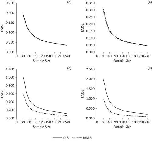
Figure 2. EMSE comparison of OLS and AWLS estimators for the case of severe heteroscedasticity (δ = 100).

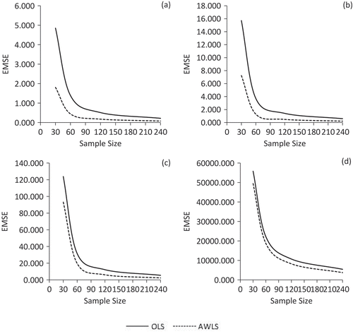
The results for the case of severe heteroscedasticity are presented in Figure 2 for discussion purpose. In Figure 2, (a), (b), (c) and (d) are used for λ = 0.80, 0.90, 0.95 and 0.99, respectively. A dramatic increase in the EMSE of both estimators is observed with the increase in collinearity level. However, the AWLSE yields lower EMSE for all collinearity levels. Moreover, the difference in the EMSE of both estimators reduces with the increase in collinearity levels.

Tables 1 and 2 present the EMSE of OLSE and AWLSE when the probability distribution of error term is t(6) and F(4, 16). Almost similar performance of the AWLSE can be observed as it exhibits in case of normal errors, when the probability distribution of error term is t(6) and F(4, 16). Efficiency of the AWLSE improves further when the error term is not only heteroscedastic but it is also non-normal, especially when the probability distribution of error term is standardized F(4, 16). For example, when T = 30 and λ = 0.50, the gain in efficiency when using the AWLSE is 70.78%, 74.29% and 103.18 for the errors distributed as N(0, 1), t(6) and F(4, 16), respectively, if the heteroscedasticity is mild (δ = 36) while the corresponding figures about gain in efficiency are 106.75%, 110.60% and 161.12% for severe heteroscedasticity (δ = 100). This shows that the AWLSE gives better performance not only in case of normal error distribution but also in case of non-normal error distribution.

Table 1. Estimated MSE when the distribution of error term is t (6)

		T = 30		T = 60		T = 120		T = 240
δ	λ	OLSE	AWLSE	OLSE	AWLSE	OLSE	AWLSE	OLSE	AWLSE
1	0.5	0.193	0.195	0.108	0.107	0.061	0.060	0.034	0.034
	0.8	0.275	0.276	0.122	0.122	0.057	0.057	0.030	0.029
	0.9	0.482	0.481	0.171	0.171	0.078	0.078	0.038	0.038
	0.95	0.934	0.934	0.331	0.330	0.145	0.145	0.070	0.069
	0.99	5.025	5.021	2.360	2.370	1.178	1.173	0.594	0.591
4	0.5	0.304	0.279	0.153	0.141	0.083	0.077	0.046	0.042
	0.8	0.524	0.458	0.199	0.177	0.091	0.083	0.044	0.040
	0.9	1.124	1.008	0.361	0.322	0.155	0.139	0.072	0.065
	0.95	3.431	3.134	1.082	0.974	0.465	0.421	0.221	0.199
	0.99	71.884	70.591	33.366	32.608	16.270	15.825	8.327	8.012
36	0.50	0.971	0.557	0.433	0.237	0.224	0.123	0.111	0.062
	0.80	2.267	1.057	0.647	0.297	0.268	0.130	0.119	0.062
	0.90	6.269	3.293	1.572	0.746	0.632	0.313	0.284	0.143
	0.95	37.958	27.505	9.877	5.915	3.869	2.117	1.799	0.956
	0.99	6446.416	5791.508	2735.119	2392.582	1274.422	1073.566	655.787	525.404
100	0.50	1.903	0.903	0.816	0.330	0.406	0.159	0.198	0.076
	0.80	4.828	1.827	1.333	0.420	0.506	0.165	0.208	0.074
	0.90	15.759	7.384	3.615	1.247	1.335	0.455	0.590	0.204
	0.95	125.305	91.919	30.224	18.189	11.922	5.854	5.609	2.262
	0.99	53689.101	45107.095	22174.257	18116.721	10565.691	8055.439	5328.479	3661.637

Table 2. Estimated MSE when the distribution of error term is F (4, 16)

		T = 30		T = 60		T = 120		T = 240
δ	λ	OLSE	AWLSE	OLSE	AWLSE	OLSE	AWLSE	OLSE	AWLSE
1	0.5	0.192	0.182	0.108	0.102	0.061	0.058	0.034	0.033
	0.8	0.270	0.255	0.121	0.114	0.059	0.056	0.030	0.029
	0.9	0.481	0.459	0.176	0.167	0.079	0.075	0.038	0.036
	0.95	0.951	0.897	0.323	0.308	0.144	0.137	0.069	0.066
	0.99	5.036	4.712	2.393	2.243	1.138	1.079	0.576	0.553
4	0.5	0.310	0.256	0.156	0.132	0.086	0.075	0.045	0.041
	0.8	0.524	0.426	0.200	0.168	0.091	0.079	0.044	0.039
	0.9	1.141	0.942	0.352	0.296	0.155	0.132	0.073	0.063
	0.95	3.501	2.818	1.048	0.877	0.465	0.394	0.219	0.189
	0.99	72.928	59.099	32.366	26.854	16.249	13.883	8.186	7.267
36	0.50	0.987	0.486	0.434	0.222	0.227	0.117	0.113	0.061
	0.80	2.303	0.940	0.676	0.283	0.267	0.127	0.115	0.060
	0.90	6.294	2.698	1.566	0.688	0.623	0.294	0.279	0.138
	0.95	37.189	18.136	9.699	4.472	3.940	1.885	1.787	0.916
	0.99	6249.723	4670.829	2720.571	2072.891	1321.113	1025.585	658.026	520.898
100	0.50	1.859	0.712	0.808	0.311	0.396	0.154	0.202	0.074
	0.80	4.919	1.414	1.303	0.369	0.499	0.161	0.203	0.075
	0.90	15.534	4.733	3.588	1.037	1.331	0.436	0.585	0.201
	0.95	124.158	58.423	30.475	12.390	12.207	4.732	5.439	2.074
	0.99	53254.592	38561.980	22147.056	16036.061	10442.854	7589.005	5283.999	3823.584

Moreover, it is observed that the level of collinearity and the degree of heteroscedasticity has a negative effect on the EMSE of both estimators (the OLSE and AWLSE). The EMSE of both estimators tends to increase with the increase in level of collinearity and degree of heteroscedasticity. On the other hand, the stated EMSE decreases as the sample size grows. The probability distribution of errors has almost similar effect on the EMSE of both estimators but the gain in efficiency of the AWLSE is the largest when the errors are F(4, 16).

4. Conclusion

This study is focused to estimate the DLM plagued with the heteroscedasticity of unknown form. One of the most popular technique, which is used for estimating the parameters of the DLM, is proposed by Almon (1965). In Almon technique, the DLM is transformed under the assumption that lag coefficients lie on a polynomial of some suitable degree and then the OLS is applied on the transformed model. If the error term is homoscedastic, there is no hindrance in applying the OLS to the transformed model but in presence of heteroscedastic errors, the OLSE for the transformed model may become seriously inefficient. Based on the work of Carroll (1982) we have proposed an adaptive estimator combined with the Almon technique, which is more efficient as compared to the conventional Almon estimator, which is based on the OLS. A Monte Carlo experiment is conducted and the AWLSE is compared with the conventional OLSE for the Almon technique, using the MSE criterion. The estimators are evaluated by varying degree of heteroscedasticity, degree of collinearity, sample size and probability distribution for the error term. The simulation results reveal that the proposed estimator (AWLSE) is an attractive choice for being more efficient over the conventional Almon OLSE in the presence of heteroscedasticity of unknown form.

Additional information

Funding

The author received no direct funding for this research.

Notes on contributors

Muhammad Aslam

Muhammad Aslam is a tenured associate professor at the Department of Statistics, Bahauddin Zakariya University, Multan, Pakistan. He acquires a teaching experience of more than 20 years at postgraduate level. His main area of interest revolves around the inference of linear regression models, including the distributed lag model (DLM) and panel data model (PDM), with issues of heteroscedasticity and multicollinearity. He has conducted a number of researches in the stated area while leading a research team, comprising of his research students and few colleagues. Recently, this team has developed three R packages, namely “mctest,” “lmridge,” and “liureg” which are available on the R CRAN. These are comprehensive packages for detection of multicollinearity, estimation of the ridge and Liu regression models with different choices of penalties. This paper is a part of PhD research project of Mr. Abdul Majid (the Principal author) under the supervision of Dr. Aslam. This paper also suggests some efficient estimation the DLM in the presence of heteroscedasticity.

References

- Ahmed, M., Aslam, M., & Pasha, G. R. (2011). Inference under heteroscedasticity of unknown form using an adaptive estimator. Communication in Statistics-Theory and Methods, 40(24), 4431–4457. doi:10.1080/03610926.2010.513793
- Alheety, M. I., & Kibria, B. M. G. (2009). On the Liu and almost unbiased Liu estimators in the presence of multicollinearity with heteroscedastic or correlated errors. Surveys in Mathematics and Its Applications, 4, 155–167.
- Alkhamisi, M., Khalaf, G., & Shukur, G. (2006). Some modifications for choosing ridge parameters. Communication in Statistics-Theory and Methods, 35(11), 2005–2020. doi:10.1080/03610920600762905
- Almon, S. (1965). The distributed lag between capital appropriations and expenditures. Econometrica : Journal of the Econometric Society, 33(1), 178–196. doi:10.2307/1911894
- Aslam, M. Adaptive procedures for estimation of linear regression models with known and unknown heteroscedastic errors (Ph.D. thesis), Bahauddin Zakariya University, Multan, Pakistan, 2006.
- Aslam, M. (2014). Performance of Kibria’s method for the heteroscedastic ridge regression model: Some monte carlo evidence. Communication in Statistics-Simulation and Computation, 43(4), 673–686. doi:10.1080/03610918.2012.712185
- Aslam, M., Riaz, T., & Altaf, S. (2013). Efficient estimation and robust inference of linear regression models in the presence of heteroscedastic errors and high leverage points. Communications in Statistics - Simulation and Computation, 42(10), 2223–2238. doi:10.1080/03610918.2012.695847
- Baltagi, B. H. (2011). Econometrics (5th ed.). Berlin: Springer.
- Carroll, R. J. (1982). Adapting for heteroscedasticity in linear models. Annals of Statistics, 10(4), 1224–1233. doi:10.1214/aos/1176345987
- Carroll, R. J., & Ruppert, D. (1982). Robust estimations in heteroscedastic of linear models. Annals of Statistics, 10(2), 429–441. doi:10.1214/aos/1176345784
- Cribari-Neto, F. (2004). Asymptotic inference under heteroscedasticity of unknown form. Computational Statistics & Data Analysis, 45(2), 215–233. doi:10.1016/S0167-9473(02)00366-3
- Cribari-Neto, F., & Da Silva, W. B. (2011). A new heteroskedasticity-consistent covariance matrix estimator for the linear regression model. AStA Advances in Statistical Analysis, 95(2), 129–146. doi:10.1007/s10182-010-0141-2
- Delgado, M. A. (1992). Semiparametric generalized least squares estimation in the multivariate nonlinear regression model. Econometric Theory, 8, 203–222. doi:10.1017/S0266466600012767
- Fair, C. R., & Jaffee, M. D. (1971). A note on the estimation of polynomial distributed lags. Econometric research program research memorandum. (No:120). University of California, Berkeley School of Law.
- Frost, P. A. (1975). Some properties of the Almon lag technique when one searches for degree of polynomial and lag. Journal of the American Statistical Association, 70(351), 606–612.
- Fuller, W. A., & Rao, J. N. K. (1978). Estimation for a linear regression model with unknown diagonal covariance matrix. Annals of Statistics, 6(5), 1149–1158. doi:10.1214/aos/1176344317
- Gibbons, D. G. (1981). A simulation study of some ridge estimators. Journal of American Statistical Association, 76(373), 131–139. doi:10.1080/01621459.1981.10477619
- Gujarati, D. N. (2003). Basic Econometrics (4th ed.). New York: McGraw-Hill.
- Güler, H., Gültay, B., & Kaçiranlar, S. (2017). Comparisons of the alternative biased estimators for the distributed lag models. Communication in Statistics-Simulation and Computation, 46(4), 3306–3318. doi:10.1080/03610918.2015.1053919
- Judge, G. G., Griffiths, W. E., Hill, R. C., Lütkepohl, H., & Lee, T. C. (1980). The theory and practice of econometrics. New York, NY: Wiley Publication.
- Kibria, B. M. G. (2003). Performance of some new ridge regression estimators. Communications in Statistics - Simulation and Computation, 32(2), 419–435. doi:10.1081/SAC-120017499
- Koyck, L. M. (1954). Distributed lags and investment analysis. Amsterdam: North Holland Publishing Company.
- Lawless, J. F., & Wang, P. (1976). A simulation study of ridge and other regression estimators. Communications in Statistics A, 5(4), 307–323. doi:10.1080/03610927608827353
- Maddala, G. S. (1977). Econometrics. New York: McGraw-Hill.
- Månsson, K., Shukur, G., & Kibria, B. M. G. (2010). A simulation study of some ridge regression estimators under different distributional assumptions. Communication in Statistics-Simulation and Computation, 39(8), 1639–1670. doi:10.1080/03610918.2010.508862
- Nadaraya, E. A. (1964). On estimating regression. Theory Probability and Its Applications, 9(1), 141–142. doi:10.1137/1109020
- Özbay, N., & Kaçıranlar, S. (2017). The Almon two parameter estimator for the distributed lag models. Journal of Statistical Computation and Simulation, 87(4), 834–843. doi:10.1080/00949655.2016.1229317
- Özbay, N., Kaçıranlar, S., & Dawoud, I. (2017). The feasible generalized restricted ridge regression estimator. Journal of Statistical Computation and Simulation, 87(4), 753–765. doi:10.1080/00949655.2016.1224880
- Pasha, G. R. Estimation methods for regression models with unequal error variances (Ph.D. thesis), University of Warwick, Coventry, Warwick, U.K, 1982.
- Robinson, P. M. (1987). Asymptotically efficient estimation in the presence of heteroscedasticity of unknown form. Econometrica : Journal of the Econometric Society, 55(4), 875–891. doi:10.2307/1911033
- Roy, N. (2002). Is adaptive estimation useful for panel models with heteroskedasticity in the individual specific error component? Some Monte Carlo evidence. Econometric Reviews, 21, 189–203. doi:10.1081/ETC-120014348
- Shiller, R. J. (1973). A distributed lag estimator derived from smoothness priors. Econometrica : Journal of the Econometric Society, 41(4), 775–788. doi:10.2307/1914096
- Silverman, B. W. (1998). Density estimation for statistics and data analysis. London: Chapman & Hall/CRC.
- Vinod, H. D., & Ullah, A. (1981). Recent advances in regression methods. New York: Marcel Dekker.
- Watson, G. S. (1964). Smooth regression analysis. Sankhya A, 26(4), 359–372.