Improved methods for estimating fraction of missing information in multiple imputation¹

1. The findings and conclusions in this report are those of the authors and do not necessarily represent the official position of the National Center for Health Statistics (NCHS) or Centers for Disease Control (CDC), USA.

Abstract

Multiple imputation (MI) has become the most popular approach in handling missing data. Closely associated with MI, the fraction of missing information (FMI) is an important parameter for diagnosing the impact of missing data. Currently γ_m, the sample value of FMI estimated from MI of a limited m, is used as the estimate of γ₀, the population value of FMI, where m is the number of imputations of the MI. This FMI estimation method, however, has never been adequately justified and evaluated. In this paper, we quantitatively demonstrated that E(γ_m) decreases with the increase of m so that E(γ_m) > γ₀ for any finite m. As a result γ_m would inevitably overestimate γ₀. Three improved FMI estimation methods were proposed. The major conclusions were substantiated by the results of the MI trials using the data of the 2012 Physician Workflow Mail Survey of the National Ambulatory Medical Care Survey, USA.

Keywords:

• fraction of missing information
• multiple imputation
• missing data
• National Ambulatory Medical Care Survey
• number of imputations

PUBLIC INTEREST STATEMENT

In any big surveys such as the National Ambulatory Medical Care Survey, USA, you select people into your sample and ask them to answer your questions. Some will answer, and others will not answer. When you finally get your survey data, it is inevitable that you will have missing data due to those non-respondents. How to minimize the effects of the missing data on your survey has been a big topic in statistics. Multiple imputation (MI) has become the most popular approach in handling missing data. Closely associated with MI, the fraction of missing information (FMI) is an important parameter for diagnosing the impact of missing data. This paper shows that the current method for estimating FMI bears intolerable biases. We proposed three improved methods that would give more accurate estimate of FMI.

1. Introduction

Multiple imputation (MI) becomes the most popular approach to accounting for missing data (Carpenter & Kenward, 2013, Dohoo, 2015, Rezvan, Lee, & Simpson, 2015, Rubin, 1987, Van Buuren, 2012). Closely associated with MI, fraction of missing information (FMI) is an important parameter for diagnosing the effects of data missingness (Rubin, 1987). FMI can be interpreted as the fraction of information about Q due to non-response, where Q is the quantity of interest (Rubin, 1987). As MI become increasingly important, the importance of FMI is also increasing. The best known use of FMI is to define the relative efficiency (RE) of MI as RE = (1 + γ₀/m)^−1/2, where γ₀ is the population value of FMI and m is the number of imputations (Rubin, 1987). Based on this RE, Rubin concluded that m ≤ 5 would be sufficient for MI (Rubin, 1987). Little et al. as well as Wagner suggested that FMI be used as an alternative tool for measuring data missing data or the response rate (Little et al., 2016, Wagner, 2010). Siddique, Harel, Crespic, and Hedekerd (2014) used FMI to verify the missing data mechanisms. The most common practice of FMI estimation is to use γ̂₀ = γ_m, where γ̂₀ is the estimated value of γ₀ and γ_m is the FMI obtained from MI of a given m, e.g. (Khare, Little, Rubin, & Schafer, 1993, Lewis et al., 2014, Schafer, 2001, Schenker et al., 2006). However, the accuracy of the γ̂₀ = γ_m method has not been adequately evaluated. This paper is to quantify possible biases of γ̂₀ = γ_m and to improve FMI estimation methodology if necessary and possible.

Established by Rubin in 1987, the current FMI paradigm is defined by Equations (1)–(11) below:

(1) ${\bar{Q}}_m=\frac{1}{m}\sum _m^1{Q}_i,$(1)

where subscript m and ∞ stands for a finite and infinite m, the subscript 0 for the population value, the subscript i for the ith imputation, and the bar hat for the parameter’s mean.

(2) $B_m=\frac{1}{m-1}\sum _1^m{\left(Q_i-{\bar{Q}}_m\right)}^2$(2)

(3) $U_m=\frac{1}{m}\sum _1^m{U}_i$(3)

(4) $T_m=U_m+\left(1+\frac{1}{m}\right)B_m,$(4)

where B, U, and T are the between-imputation, within-imputation, and the total variances.

(5) $r=\left(1+\frac{1}{m}\right)\frac{B_m}{U_m},$(5)

where $r$ is the fractional variance increase due to data missingness.

(6) $v=\left(m-1\right){\left(1+\frac{1}{r}\right)}^2,$(6)

where $v$ is the degrees of freedom.

(7) ${\gamma }_m=\frac{r+2/\left(v+3\right)}{r+1}$(7)

(8) $T_{\mathrm{\infty }}=U_{\mathrm{\infty }}+B_{\mathrm{\infty }}$(8)

(9) ${\gamma }_{\mathrm{\infty }}=\frac{B_{\mathrm{\infty }}}{T_{\mathrm{\infty }}}$(9)

(10) $T_0=U_0+B_0$(10)

(11) ${\gamma }_0=\frac{B_0}{T_0}.$(11)

Equation (11) cannot be used to calculate γ₀ in practice because B₀, U₀, and T₀ are usually unknown. No researchers have provided an equation that explicitly links γ_m and γ₀. The justification for using γ̂₀ = γ_m is not available from Equations (1)–(11).

Assume γ_∞ = γ₀. For γ̂₀ = γ_m to be valid, E(γ_m) = γ₀ must be true. For E(γ_m) = γ₀ to be true, E(γ_m) must be independent of m. To understand E(γ_m), let the same MI of a given m be repeated for j times. Denote the γ_m from each MI repeat as γ_m1, γ_m2, γ_m3, …, γ_mj. By definition, the expected value is the sum of all possible values each multiplied by the probability of its occurrence (Hogg, McKean, & Craig, 2013). Therefore, E(γ_m) can be defined as:

(12) $E\left({\gamma }_m\right)=\underset{j\to \mathrm{\infty }}{lim}\left(\frac{1}{j}\sum _j^1{\gamma }_{mj}\right).$(12)

Equation (12) shows that E(γ_m) can be understood as the ultimate mean of γ_m when j becomes infinity. If E(γ_m) is independent of m, we should have E(γ₂) = E(γ₃) = … = E(γ_m) = γ₀, and the use of ${\hat{\gamma }}_0$ = γ_m would be justified. If E(γ_m) depends on m, we should have E(γ₂) ≠ E(γ₃) ≠ … ≠ E(γ_m) ≠ γ₀. The use of γ̂₀ = γ_m may not be justified if the difference between E(γ_m) and γ₀ is intolerably big.

Rubin indicated that the mean of γ_m can be regarded as γ₀ [1 page 143], underlining an assumption that E(γ_m) is independent of m. Harel briefly mentioned that γ_m “tends to decrease as m increases” without providing any details (Harel, 2007). Although Harel’s statement favours E(γ_m) ≠ γ₀, it cannot be a base for disproving γ̂₀ = γ_m because it might be acceptable to use γ̂₀ = γ_m if the decrease of γ_m with the increase of m is statistically negligible. To date the justifications for using γ̂₀ = γ_m is still missing.

For FMI estimation, Harel’s 2007 paper (Harel, 2007) is important in that it pointed out that, unlike γ_m that “tends to decrease as m increases,” the quantity B_m/(U_m + B_m) “does not tend to decrease as m increases” (Harel, 2007). Harel used γ̂₀ = B_m/(U_m + B_m) to estimate FMI in his research (Harel, 2007). The goal of Harel’s paper was not to find a better FMI estimation method per se and his discussion on γ̂₀ = B_m/(U_m + B_m) was brief. Most researchers have not used Harel’s method for FMI estimation probably because most people may have treated Harel’s method as being research-specific rather than a method that may potentially be universally used for FMI estimation.

In this study, we examined the relationships between m, γ_m, γ_∞, and γ₀, quantified the decrease of γ_m with the increase of m, quantified the biases of γ̂₀ = γ_m, and proposed improved methods for FMI estimation. Only univariate FMI definition will be examined in this paper even though multivariate FMI definition may exist. The major conclusions were substantiated by the MI trials using the data of the 2012 Physician Workflow Mail Survey (PWS) of the National Ambulatory Medical Care Survey (NAMCS). This paper focuses on MI approach only even though it may be possible to estimate FMI via a non-MI approach (Savalei & Rhemtulla, 2012, Zheng & Lo, 2008).

2. The relationships between m, γ_m, γ_∞, and γ₀

2.1. The condition for γ_∞ = γ₀

To use γ_m for estimating γ₀, one must assume γ_∞ = γ₀. Most researchers simply treat γ_∞ and γ₀ as synonyms (e.g. He et al., 2016). But they are not. Imagine a population of imputations (POI) is generated by repeating the imputation of the same model on the same data for an infinite number of times. An MI is simply a sample of the POI with sample size m. The sample value and the population value of FMI for the POI are γ_m and γ_∞, respectively. The population for γ₀, however, is not POI but the population of the sampling units of the survey. A γ_∞ is inseparably linked to an MI, but a γ₀ can be independent of MI. The γ₀ may be estimated by MI as well as other methods such as maximum likelihood (Savalei & Rhemtulla, 2012, Zheng & Lo, 2008). Using Equations (5)–(7), one can prove that the condition for γ_∞ = γ₀ is B_m/U_m = B₀/U₀. When we use MI to estimate γ₀, we have to assume γ_∞ = γ₀, which is probably why γ_∞ and γ₀ are often treated as synonyms in MI analyses. In this paper, we will assume γ_∞ = γ₀ because we use MI to estimate γ₀.

2.2. B_m/U_m is independent of m

Equation (7) that defines γ_m does not have m as a factor. Combining Equations (5), (6), and (7) gives an expanded definition of γ_m with m as one of the independent factors affecting γ_m:

(13) ${\gamma }_m=\frac{\left(1+\frac{1}{m}\right)\frac{B_m}{U_m}+2/\left(\left(m-1\right){\left(1+\frac{1}{\left(1+\frac{1}{m}\right)\frac{B_m}{U_m}}\right)}^2+3\right)}{\left(1+\frac{1}{m}\right)\frac{B_m}{U_m}+1}.$(13)

Equation (13) shows that γ_m is a function of three factors, i.e. γ_m = F(m, B_m, U_m). In Equation (13), B_m and U_m always appear together as B_m/U_m. Letting c_m = B_m/U_m, then γ_m becomes a function of two factors, i.e. γ_m = F(m, c_m).

Whether c_m is independent of m is important in understanding the m–γ_m relationship. If c_m depends on m, the direct effects of m on γ_m would be confounded by the indirect effects of m on γ_m via m’s effects on c_m, which in turn could be due to m’s effect on B_m, U_m or both. If c_m is independent of m, then the m–γ_m relationship would be greatly simplified.

In order to establish that c_m is independent of m, we need to prove E(B_m/U_m) = B₀/U₀. Equation (2) indicates that the relationship between m and B_m is that between the sample size n and the variance (s²) so that E(B_m) is independent of m, i.e. E(B_m) = B₀ (Serfling, 1980). Equation (3) indicates that the relationship between m and U_m is that between the sample size n and the sample mean x̅ so that E(U_m) is independent of m, i.e. E(U_m) = U₀ (Hogg et al., 2013). Jensen’s Inequality (Hogg et al., 2013) determines that E(1/U_m) ≥ 1/E(U_m). Therefore E(B_m/U_m) = E(B_m)E(1/U_m) ≥ E(B_m)/E(U_m) = B₀/U₀, or E(B_m/U_m) ≥ B₀/U₀. Our simulation studies show that the maximum difference between E(B_m)/E(U_m) and E(B_m/U_m) is less than 0.1%, which is negligible in virtually any statistics work. We can safely regard E(B_m/U_m) = B₀/U₀ as a fact for the purpose of studying the m–γ_m relationship. The c_m’s independence of m is thus proved. The subscript m can be removed from c_m. As a result, we can indeed letting c_m = B_m/U_m be a constant c in Equation (13) and make γ_m become a function of the single factor m, i.e. γ_m = F(m).

2.3. The γ_m = F(m,γ₀) equation

When m goes infinite, γ_m becomes γ₀. Our goal is to establish the mathematic relationship between γ_m and γ₀ at a finite m, which is currently missing in published literatures. In the discussions above, we have showed that it is mathematically legitimate to letting c_m be a constant c in studying the m–γ_m relationship because c_m is independent of m. What is the best value to choose for c to obtain the most truthful m–γ_m relationship? The answer is: c = E(B_m/U_m) = B₀/U₀. If and only if c = E(B_m/U_m) = B₀/U₀, the m–γ_m relationship as determined by Equation (13) would reflect the true m–γ_m relationship. From Equations (10) and (11) we can obtain B₀/U₀ = γ₀/(1 − γ₀). Replacing B_m/U_m in Equation (13) with γ₀/(1 − γ₀), we obtain an equation that directly links γ_m to γ₀ as follows:

(14) ${\gamma }_m=E\left({\gamma }_m\right)=F\left(m,{\gamma }_0\right)=\frac{\left(1+\frac{1}{m}\right)\frac{{\gamma }_0}{1-{\gamma }_0}+2/\left(\left(m-1\right){\left(1+\frac{1}{\left(1+\frac{1}{m}\right)\frac{{\gamma }_0}{1-{\gamma }_0}}\right)}^2+3\right)}{\left(1+\frac{1}{m}\right)\frac{{\gamma }_0}{1-{\gamma }_0}+1}.$(14)

Establishment of equation is a significant step forward in understanding the relationship between m, γ_m, and γ₀ because it links the three factors in the same equation for any m, finite or infinite.

For a given analysis of a given dataset, γ₀ is a constant. When we repeat the same MI of a given m for j times, the γ_m value from each repeat of the MI will not change when the γ_m is determined by Equation (14). In other words, we will have γ_m1 = γ_m2 = γ_m3 = … γ_mj = E(γ_m) (see Equation (12)). In other words, the γ_m value obtained from Equation (14) will be E(γ_m). For different data and analyses, γ₀ is a variable. Equation (14) shows that E(γ_m) is a function of the two factors, m and γ₀, i.e. E(γ_m) = F(m, γ₀).

3. The decrease of E(γ_m) with the increase of m

3.1. E(γ_m) > γ₀ for any finite m

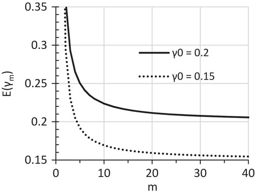
We all know that E(x̅) is independent of n and equals to μ, which provides the theoretical base for μ̂ = x̅ (Hogg et al., 2013). The use of γ̂₀ = γ_m implies the assumption that E(γ_m) = γ₀. Using Equation (14), the m–E(γ_m) relationship curve can be constructed for any given γ₀. Figure 1 presents the m–E(γ_m) relationship curves for γ₀ = 0.15 and 0.2. Based on Figure 1, for the first time in MI research, we can explicitly state this important fact: E(γ_m) decreases with the increase of m. The decrease of E(γ_m) with the increase of m can be interpreted as follows: For a given dataset with a given MI model, the ultimate mean of γ_m, which is the mean of an infinite number of individual γ_m values obtained from repeating the MI of the given m for an infinite number of times, would always be greater than the γ₀. Of course what is called “the ultimate mean” here is the E(γ_m) (Hogg et al., 2013). Therefore, by showing E(γ_m) decreases with the increase of m, we have proved that E(γ_m) > γ₀ for any finite m (Figure 1). The fact that E(γ_m) > γ₀ is further illustrated by more data in Table 1 for a wider range of m values and more γ₀ values.

Table 1. Changes of E(γ_m), D_γ, and R_Dγ with the increase of m at different γ₀ levels, where D_γ = 100(E(γ_m)−γ₀)/γ₀ and R_Dγ = 100(γ_m−γ_m+1)/γ_m+1

m	E(γm)		RDγ		Dγ
	γ0 = 0.2	γ0 = 0.01	γ0 = 0.2	γ0 = 0.01	γ0 = 0.2	γ0 = 0.01
2	0.361	0.01536	23.33	14.12	80.59	53.64
5	0.250	0.01205	3.872	2.957	25.23	20.47
10	0.224	0.01102	1.0240	0.8502	11.84	10.16
20	0.212	0.01051	0.2664	0.2306	5.750	5.062
40	0.206	0.01025	0.0682	0.0602	2.837	2.528
60	0.204	0.01017	0.0306	0.0272	1.883	1.684
100	0.202	0.01010	0.0111	0.0099	1.126	1.010
200	0.201	0.01005	0.0028	0.0025	0.561	0.505

Figure 1. The m–E(γ_m) relationship curve at γ₀ = 0.2 and 0.15 as determined by Equation (14).

3.2. The bias of the current FMI estimation method

The fact that E(γ_m) > γ₀ dictates that the current FMI estimation method γ̑₀ = γ_m must be biased. One achievement of this paper is that we successfully quantified the bias of the current FMI estimation method. We use D_γ, the percentage difference between E(γ_m) and γ₀ as the parameter to measure this bias, i.e.:

(15) $D_{\gamma }=100\frac{{\gamma }_m-{\gamma }_0}{{\gamma }_0}.$(15)

Table 1 presents the D_γ values at different γ₀ and m values as determined by Equation (14). At a given m, D_γ differs at different γ₀ values (Table 1). For m = 2, D_γ is 80.59% and 53.64% for γ₀ = 0.2 and 0.01, respectively (Table 1). When γ₀ increased from 0.001 to 0.6, D_γ first increases with the increase of γ₀, reaches a peak, and then decreases (Table 1 and Figure 2). The value of the γ₀ at which D_γ reaches the peak differs with m (data not shown). For m = 5, the maximum D_γ value of 25.31% occurs at γ₀ = 0.23, and the minimum D_γ value of 16.53% occurs at γ₀ = 0.6 (Figure 2(b)). In other words, one could overestimate FMI by 25% at m = 5 if the current method is used. A bias of this magnitude cannot and should not be ignored. Development of a better FMI estimation method is indeed necessary.

Figure 2. Effects of γ₀ levels on D_γ as defined by Equation (15) and R_Dγ as defined by Equation (16): a. D_γ at m = 5; b. D_γ at m = 2.

3.3. The γ_m decrease rate: smaller at larger m

We use R_γd, the percentage rate of the γ_m decrease per unit m, to measure the rate of the γ_m decrease:

(16) $R_{D\gamma }=100\frac{{\gamma }_m-{\gamma }_{m+1}}{{\gamma }_{m+1}}.$(16)

R_Dγ is affected by both m and γ₀ (Table 1 and Figure 2, b1 and b2). At m = 5, R_Dγ is 3.87% and 2.96% for γ₀ = 0.2 and 0.01, respectively (Table 1). Figure 2(b) show that R_Dγ increases initially, reaches a peak, and then decreases as γ₀ increases from 0.001 to 0.6. For m = 2, the maximum R_Dγ = 23.91% occurs at γ₀ = 0.15 (Figure 2(b)). For m = 5, the maximum R_Dγ = 3.88% occurs at γ₀ = 0.21 (data not shown). The gradual reduction of R_Dγ makes it possible for choosing a sufficient m when the m-driven γ_m reduction becomes negligibly small.

4. Improved methods for γ₀ estimation

Regarding γ̂₀ = γ_m as the control, any method that gives more accurate FMI estimation than this control will be considered as an improved method. Three improved methods are proposed below.

4.1. Improved method 1: γ̂₀ = γ_m≥100

The control method is to use γ̂₀ = γ_m regardless the size of m. The first improved method is to choose a sufficiently large m when use γ̂₀ = γ_m. Data in Figure 1 show that E(γ_m) approaches γ₀ as m gets larger. Therefore, γ_m would estimate γ₀ with an adequate accuracy when m is sufficiently large. Various criteria have been used to determine the sufficient m (Bodner, 2008, Graham, Olchowski, & Gilreath, 2007, Hershberger & Fisher, 2003, Pan, Wei, Shimizu, & Jamoom, 2014, Royston, 2004, Rubin, 1987). An adequately accurate estimation of γ₀ using γ̂₀ = γ_m offers another criterion for determining a sufficient m. As measured by R_Dγ, the gain in reducing the bias from increasing a unit m becomes smaller at a greater m. Using Equation (14), we can prove the bias of the default method as measured by D_γ would be about 1% or less for any reasonable γ₀ values when m is greater than 100. We arbitrarily choose a bias of ≤1% as an acceptable level and recommend m ≥100 as being sufficient for an adequately accurate estimation of γ₀ using γ̂₀ = γ_m. This method can be expressed as γ̂₀ = γ_m≥100.

4.2. Improved method 2: γ̂₀ = γ_m(m/(m + 1))

Calculating γ_m for different m and γ₀ combinations using Equation (14), one will find the following approximation stands well for m ≥10:

(17) ${\gamma }_m\approx \frac{m+1}{m}{\gamma }_0.$(17)

From Equation (17), we obtain the following method of estimating γ₀ from γ_m:

(18) ${\hat{\gamma }}_0=\frac{m}{m+1}{\gamma }_m.$(18)

For those who may be interested, this method may be proven by resolving γ₀ from Equation (14) using Taylor series expansion approximation. An advantage of this method is that one could use it to have a more accurate FMI estimation from the m and the γ_m information available in an earlier publication that uses a small m and γ_m to estimate FMI.

4.3. Improved method 3: γ̂₀ = c_m/(c_m + 1), where c_m = B_m/U_m

In Section 2.2, we proved that E(B_m/U_m) = B₀/U₀. In other words, B_m/U_m is an unbiased estimation of B₀/U₀. As a result, Equation (19) below is a better γ₀ estimation than γ̂₀ = γ_m:

(19) ${\hat{\gamma }}_0=\frac{c_m}{1+c_m}.$(19)

where c_m = B_m/U_m. Harel used this method to estimate γ₀ for his study on two-stage MI (Harel, 2007). However, the justification for this method discussed here was not available in Harel’s paper or any other published literature (Harel, 2007).

5. Results from MI trials of PWS12

5.1. Methods

PWS was a supplemental survey of NAMCS, which collects data about the provision and use of ambulatory medical care services in the United States (Lau, McCaig, & Hing, 2016). The 2012 PWS data (PWS12) were used for the MI trial, which had 2,567 responded physicians in the sample. PWS data can be accessed via NCHS Research Data Center (RDS) program (https://www.cdc.gov/rdc/index.htm).

MI was conducted on three variables representing the physician’s practice size at different scales, namely SIZE100, SIZE20, and SIZE5. The three variables had the same missing data percentage of 29% due to item non-responses. The hot-deck imputation method (Andridge & Little, 2010) was used. The RDS-released PWS12 data, which had 3.6% of missing values for SIZE after some of the missing values in PWS12 were replaced by the corresponding non-missing values for the same physician from the 2011 PWS data, were used as the hot-deck donor. Two MI models denoted as MI-1 and MI-2 were used. MI-1 did not use any covariate in the imputation and the non-missing replacement values for the missing value were randomly chosen from entire donor dataset. MI-2 used PRIMEMM as the covariate in the imputation and the non-missing replacement values for the missing value were randomly chosen from the cell of the same PRIMEMM value in donor dataset. PRIMEMM was the physician’s primary employment type that was coded into nine categories for this research. The MIs had m = 3, 5, 10, 20, 30, 40, 60, 80, and 100, with each MI being repeated for 30 times. Excluding m, there were 12 treatment combinations (3 imputed variables × 2 imputation models × 2 analytic models). The hot-deck imputation method used in this study was similar to that used by the survey for creating the RDC-released PWS12 data. According to Rubin (1987, equation 4.3.8), the hot-deck bias can be expressed as E(B) = B(n1/n), where n is the number of the units of the full sample and n1 is the number of the units with observed values. Since the n1/n ratio is independent of m, the percentage fraction of the hot-deck bias would be a fixed value as long as the n1/n ratio is fixed. Therefore the m–γ_m relationship obtained from the hot-deck-based MI trials should still be valid. One should be aware of the potential hot-deck bias when interpreting the results of this study.

The quantity of interest (Q) was the means of the SIZE100, SIZE20, and SIZE5. Two analytical models denoted as Anal-1 and Anal-2 were used. In Anal-1, U_i, the within-imputation variance of the ith complete dataset generated by the MI, was the total variance of SIZE100, SIZE20, or SIZE5 in the ith dataset. In Anal-2, U_i was the variance of the ith dataset after the variance due to the effect of PRIMEMM was removed. Analyses were based on un-weighted data. Results obtained in this study were for research purpose only.

Barnard and Rubin (1999) suggested that, for making the statistical inferences in MI-involved analyses, instead of using the degrees of freedom ($v$) as defined by Equation (6), the adjusted degrees of freedom (DFa) as proposed by their paper should be used where the complete-data degrees of freedom is not sufficiently large. However in the γ_m definition, i.e. Equation (7), $v$ does not function as the degrees of freedom per se but mealy as a mathematical value in the estimation of γ_m. We have found that replacing $v$ in Equation (7) with DFa will result in an erroneous estimation of γ_m. Therefore we used $v$, instead of DFa, when used Equation (7) for the γ_m estimation in this study.

5.2. The γ_m decrease with the increase of m in the MI trials

Would the γ_m decrease due to the increase of m (see Section 2.1 and 3.1) be big enough to stand out from sampling errors and other noises in real-world MI analyses? The answer is yes, as demonstrated by the data in Figure 3. Figure 3 shows the effects of m on γ_m in SIZE100, SIZE20, and SIZE5 for the two MI models for Anal-2. In spite of the γ_m variations due to sampling errors as shown by the error bars in the graphs, the dominant trend was clear: γ_m decreased significantly as m increased from 3 to 100. The γ_m values at m = 3–40 were significantly greater than γ₁₀₀ in most cases (Figure 3). These results suggest that the γ_m decrease with the increase of m is not ignorable in FMI estimation in real world data analyses.

Figure 3. Effects of m on γ_m at δ = 29% for analytic model = Anal-2: a. MI model = MI-1; b. MI model = MI-2.

5.3. Variation of γ_m, B_m, and U_m

In establishing the MI framework, Rubin (1987) assumed that U_m ≈ U₀, which would be more likely to be true if the variance of U_m is negligible. The authors did not find any information on the magnitude of U_m variance in published literature. A detailed study on B_m variance was reported by Pan et al. (Pan et al., 2014). The variance of B_m was substantial when m < 30 (Pan et al., 2014). The variations in B_m and U_m would inevitably lead to γ_m variation. As a result, when using γ̑₀ = γ_m at an insufficient m, the inaccuracy of γ̑₀ would not only come from E(γ_m) > γ₀ but also from the variation of γ_m. The possible bias from sampling-error-driven γ_m variation has not been given an adequate attention.

The coefficient of variations (CV) of B_m, U_m, and γ_m are presented in Table 2. Both the imputations models and the analytic models affected the variations of γ_m, B_m, and U_m (Table 2). CV of U_m was much smaller—usually 1–10% that of B_m. The CV of B_m and γ_m were very similar, with the CV of γ_m being always slightly smaller than that of B_m. The greater the m, the smaller the variations of γ_m, B_m, and U_m (Table 2). These results were in agreement with Harel’s conclusion (Hogg et al., 2013) that it is necessary to choose a sufficient m for MI to control the variations of γ_m. Due to the significant effects of the MI model and the analytic model on the variations of γ_m, B_m, and U_m (Table 2), it may not be possible to propose a single m that fits all situations for controlling the variance of γ_m, B_m, and U_m.

Table 2. Coefficient of variations (%) of B_m, U_m, and γ_m for SIZE100

m	MI-1, Anal-1			MI-2, Anal-2
	Bm	Um	γm	Bm	Um	γm
3	20.24	0.185	20.19	1.52	0.0553	1.50
5	11.12	0.179	11.10	1.00	0.0200	1.01
10	7.75	0.135	7.75	0.88	0.0353	0.91
20	5.91	0.098	5.89	0.49	0.0282	0.48
30	6.24	0.077	6.26	0.24	0.0150	0.24
40	3.60	0.048	3.59	0.61	0.0180	0.59
60	2.74	0.058	2.73	0.39	0.0091	0.39
80	2.48	0.041	2.47	0.17	0.0062	0.17
100	2.45	0.037	2.45	0.15	0.0081	0.16

An advantage of using γ̂₀ = γ_m≥100 is that not only can this method reduce the E(γ_m) > γ₀ bias but also reduce γ_m variation because of a large m. The other two improved methods can effectively reduce or even eliminate the E(γ_m) > γ₀ bias even if when m is small. However the γ̑₀ inaccuracy may be a concern for any FMI estimation methods unless a sufficient m is chosen. Data in Figure 3 suggest that a ≥20 m may be necessary to reduce the γ_m variation to an acceptable level for using γ̂₀ = γ_m(m/(m + 1)) and γ̂₀ = c_m/(c_m + 1).

5.4. Comparison of different FMI estimation methods

Table 3 presents data for visualizing the performance of these three improved γ₀ estimation methods described in Section 4 in comparison with the default method γ̂₀ = γ_m in an example of real-world data analyses. The treatment combination of the MI trials was {SIZE20, MI-2, Anal-2}. The control values was the γ_m values at m = 3, 5, etc., which would be the FMI estimation when the default method was used. The γ₁₀₀ value was used as the γ̑₀ for the improved method γ̂₀ = γ_m≥100. The best γ̂₀ was calculated by Equation (19) using (B̅₁₀₀)/(U̅₁₀₀) as the estimate of B₀/U₀, where B̅₁₀₀ and U̅₁₀₀ were the mean of the 30 replicates of B₁₀₀ and U₁₀₀.

Table 3. Comparison of different γ₀ estimation methods for SIZE20 with imputation model = MI-2 and analytic model = Anal-2 in the PWS12 MI trials. The best γ̂₀ was calculated by Equation (19) using (B̅₁₀₀)/(U̅₁₀₀) as the estimate of B₀/U₀, where B̅₁₀₀ and U̅₁₀₀ were the mean of the 30 replicates of B₁₀₀ and U₁₀₀, respectively

m	SIZE20, MI-2, Anal-2
	Control γ̂0 = γm	Improved
		γ̂0 = γm≥100	γ̂0 = cm/(1 + cm)	γ̂0 = γm(m/(1 + m)
3	0.00379		0.00283	0.00284
5	0.00318		0.00265	0.00265
10	0.00286		0.00260	0.00260
20	0.00293		0.00279	0.00279
30	0.00278		0.00269	0.00269
40	0.00273		0.00267	0.00267
60	0.00277		0.00273	0.00273
80	0.00272		0.00269	0.00269
100	0.00270	0.00270	0.00267	0.00267
(∞)	Best γ̂0: 0.00267

For m ≤ 80, all three improved methods performed better than the control method (Table 3). These results suggest that the three improved methods proposed in this paper can be used to replace the control method in real world data analyses. In general we recommend to use γ̂₀ = c_m/(1 + c_m), for it essentially eliminates the E(γ_m) > γ₀ bias at all levels of m. But the two other methods may come in handy under certain circumstances. For example, if an earlier publication which had used m = 5 without providing B_m and U_m values, one can simply use γ̂₀ = γ_mm/(1 + m) to convert the biased γ₀ estimate of the paper into a more correct γ₀ estimate.

6. Conclusions

In most published researches, γ_∞ and γ₀ are treated as synonyms. However, the two are different. The γ₀ is independent of MI, whereas γ_∞ is a parameter of MI. γ_∞ equals to γ₀ only if B_m/U_m = B₀/U₀. To use MI for FMI estimation, one has to assume γ_∞ = γ₀, which will also be the assumption here.

The γ_m decreases with the increase of m. We quantified the m–γ_m relationship. The magnitude and the rate of the γ_m decrease varies with m and γ₀. At m = 2, γ₂ is greater than γ₀ by 50–81% depending on the γ₀ level. At m = 5, the recommended m value as being sufficient by some (e.g. Rubin, 1987), γ_m is greater than γ₀ by 20–25% when γ₀ value ranges from 0.001 to 0.6. The decrease of γ_m with the increase of m determines that E(γ_m) > γ₀ for any finite m. The results from the MI trials suggest that the volume of the γ_m decrease with increased m is not ignorable in real world data analyses in spite of the noises from sampling errors and other sources.

E(B_m) and E(U_m) are independent of m. Therefore, the decrease of γ_m with the increase of m is not due to an indirect effect of m on E(B_m) and E(U_m). As a result, it is not necessary to use the B_m and U_m from the same MI for best γ_m estimation. Instead, one should use the best estimates of B₀ and U₀ available, which leads to the development of Equation (14) that links γ_m to γ₀ directly.

The variation in γ_m can be substantial. The CV of γ_m was essentially identical with that of B_m, and CV of U_m was 1–10% that of γ_m or B_m. The variation of γ_m is smaller as m gets bigger. The inaccuracy of FMI estimation due to γ_m variation should be concerned in FMI estimation when m is small regardless what method is used.

The current method γ̂₀ = γ_m may result in a substantial FMI overestimation when m is not sufficiently large. Three improved methods are proposed for estimating γ₀ from MI of a finite m. These three methods are (1) γ̂₀ = γ_m≥100, (2) γ̂₀ = γ_m(m/(m + 1)), and (3) γ̂₀ = c_m/(c_m + 1), where c_m = B_m/U_m. In our MI trials, all three improved methods gave more accurate γ₀ estimates than γ̂₀ = γ_m where m is less than 80.

When m is sufficiently large, say, m ≥ 100, all three methods should give a statistically sound estimation of γ₀. When m is not sufficiently large, say, m < 100, the third method γ̂₀ = c_m/(c_m + 1) should be one’s best option for γ₀ estimation. The second method γ̂₀ = γ_m(m/(m + 1)) has its value where B_m and U_m are not available and the only values available to use for γ₀ estimation are m and γ_m.

Competing interests

The authors declared no potential conflicts of interest with respect to the research, authorship, and/or publication of this article.

Acknowledgements

Dr. Yulei He of NCHS is sincerely thanked for his invaluable insights and suggestions.

Additional information

Funding

This work was performed while the authors were under employment by the US federal government. The authors used government resources, e.g. computers and office spaces, for this research. The authors did not receive any specified funding for this research from inside or outside US government resources.

Notes on contributors

Qiyuan Pan

Qiyuan Pan is a mathematical statistician in Division of Health Care Statistics, National Center for Health Statistics (NCHS), Centers for Disease Control and Prevention (CDC), U.S. Department of Health and Human Services (HHS), USA. He obtained his PhD from University of Maryland, USA.

Rong Wei

Rong Wei is a mathematical statistician in Mathematical Statistics Branch, Division of Research and Methodology, NCHS, CDC, HHS. She obtained her PhD from University of Wisconsin, USA.

Notes

1. The findings and conclusions in this report are those of the authors and do not necessarily represent the official position of the National Center for Health Statistics (NCHS) or Centers for Disease Control (CDC), USA.

References

- Andridge, R. R., & Little, R. J. (2010). A review of hot deck imputation for survey non-response. International Statistical Review, 78(1), 40–64. doi:10.1111/j.1751-5823.2010.00103.x
- Barnard, J., & Rubin, D. B. (1999). Small-sample degrees of freedom with multiple imputation. Biometrika, 86(4), 948–955. doi:10.1093/biomet/86.4.948
- Bodner, T. E. (2008). What improves with increased missing data imputations? Structural Equation Modeling: A Multidisciplinary Journal, 15, 651–675. doi:10.1080/10705510802339072
- Carpenter, J., & Kenward, M. (2013). Multiple imputation and its application. John Wiley & Sons.
- Dohoo, I. R. (2015). Dealing with deficient and missing data. Preventive Veterinary Medicine, 122(1–2), 221–228. doi:10.1016/j.prevetmed.2015.04.006
- Graham, J. W., Olchowski, A. E., & Gilreath, T. D. (2007). How many imputations are really needed? Some practical clarifications of multiple imputation theory. Prevention Science, 8(3), 206–213. doi:10.1007/s11121-007-0070-9
- Harel, O. (2007). Inferences on missing information under multiple imputation and two-stage multiple imputation. Statistical Methodology, 4, 75–89. doi:10.1016/j.stamet.2006.03.002
- He, Y., Shimizu, I., Schappert, S., Xu, J., Beresovsky, V., Khan, D., … Schenker, N. (2016). A note on the effect of data clustering on the multiple-imputation variance estimator: A theoretical addendum to the Lewis et al. article in JOS 2014. Journal of Official Statistics, 32(1), 147–164. doi:10.1515/jos-2016-0007
- Hershberger, S. L., & Fisher, D. G. (2003). A note on determining the number of imputations for missing data. Structural Equation Modeling, 10(4), 648–650. doi:10.1207/S15328007SEM1004_9
- Hogg, R. V., McKean, J. W., & Craig, T. A. (2013). Introduction to mathematical statistics (7th ed.). Boston: Pearson Education, Inc.
- Khare, M., Little, R. J. A., Rubin, D. B., & Schafer, J. L. 1993. Multiple imputation of NHANES III. Proceedings of the Survey Research Methods Section, American Statistical Association, pp. 297–302.
- Lau, D. T., McCaig, L. F., & Hing, E. (2016). Toward a more complete picture of outpatient, office-based health care in the U.S: Expansion of NAMCS. American Journal of Preventive Medicine, 51(3), 403–409. doi:10.1016/j.amepre.2016.02.028
- Lewis, T., Goldberg, E., Schenker, N., Beresovsky, V., Schappert, S., Decker, S., … Shimizu, I. (2014). The relative impacts of design effects and multiple imputation on variance estimates: A case study with the 2008 National Ambulatory Medical Care Survey. Journal of Official Statistics, 30(1), 147–161. doi:10.2478/jos-2014-0008
- Little, R. J., Wang, J., Sun, X., Tian, H., Suh, E.-Y., Lee, M., … Mohanty, S. (2016). The treatment of missing data in a large cardiovascular clinical outcomes study. Clinical Trials, 13(3), 344–351. doi:10.1177/1740774515626411
- Pan, Q., Wei, R., Shimizu, I., & Jamoom, E. (2014). Determining sufficient number of imputations using variance of imputation variances: Data from 2012 NAMCS Physician Workflow Mail Survey. Applied Mathematics, 5, 3421–3430. doi:10.4236/am.2014.521319
- Rezvan, P. H., Lee, K. J., & Simpson, J. A. (2015). The rise of multiple imputation: A review of the reporting and implementation of the method in medical research. BMC Medical Research Methodology, 15, 30. doi:10.1186/s12874-015-0022-1
- Royston, P. (2004). Multiple imputation of missing values. The Stata Journal, 4(3), 227–241.
- Rubin, D. B. (1987). Multiple imputation for nonresponse in surveys. New York, NY: John Wiley & Sons.
- Savalei, V., & Rhemtulla, M. (2012). Missing information from full information maximum likelihood. Structural Equation Modeling: A Multidisciplinary Journal, 19(3), 477–494. doi:10.1080/10705511.2012.687669
- Schafer, J. L. (2001). Analyzing the NHANES III multiply imputed data set: Methods and examples. Retrieved from ftp://ftp.cdc.gov/pub/Health_Statistics/NCHS/Datasets/NHANES/NHANESIII/7a/doc/analyzing.pdf.
- Schenker, N., Raghunathan, T. E., Chiu, P.-L., Makuc, D. M., Zhang, G., & Cohen, A. J. (2006). Multiple imputation of missing income data in the national health interview survey. Journal of the American Statistical Association, 101, 924–933. doi:10.1198/016214505000001375
- Serfling, R. (1980). Approximation theorems of mathematical statistics. John Wiley & Sons, Inc.
- Siddique, J., Harel, O., Crespic, C. M., & Hedekerd, D. (2014). Binary variable multiple-model multiple imputation to address missing data mechanism uncertainty: Application to a smoking cessation trial. Statistics in Medicine, 33, 3013–3028. doi:10.1002/sim.6137
- Van Buuren, S. (2012). Flexible imputation of missing data. Boca Raton, FL: Chapman and Hall/CRC Press.
- Wagner, J. (2010). The fraction of missing information as a tool for monitoring the quality of survey data. Public Opinion Quarterly, 74(2), 223–243. doi:10.1093/poq/nfq007
- Zheng, T., & Lo, S.-H. (2008). Comment: Quantifying the fraction of missing information for hypothesis testing in statistical and genetic studies. Statistical Science, 23, 321–324. doi:10.1214/08-STS244A