Multinomial approximation to the Kolmogorov Forward Equation for jump (population) processes

Abstract

We develop a simulation method for Markov Jump processes with finite time steps based in a quasilinear approximation of the process and in multinomial random deviates. The second-order approximation to the generating function, Error = O(dt²), is developed in detail and an algorithm is presented. The algorithm is implemented for a Susceptible-Infected-Recovered-Susceptible (SIRS) epidemic model and compared to both the deterministic approximation and the exact simulation. Special attention is given to the problem of extinction of the infected population which is the most critical condition for the approximation.

Keywords:

• jump processes
• continuous-time Markov chains
• approximating methods
• multinomial processes
• Feller–Kendall algorithm
• SIRS epidemic model

PUBLIC INTEREST STATEMENT

The overall goal of population dynamics is to understand the collective time-evolution of populations in terms of their reciprocal and environmental influences. The description is made in terms of the number of individuals that share the same relevant characteristics and results in a intrinsic (unavoidable) stochasticity. This manuscript describes a new implementation of the core stochastic methods. The new method takes advantage of particularities that more often than not appear in biological populations such as in the description of biological cycles and/or the progress in time of epidemic outbreaks. The present method is more efficient than a general approach, while keeping accuracy within desirable levels. Understanding, modelling and predicting population processes is an important ingredient in the development of public policies such as health or farming, to mention just a few.

1. Introduction

In a broad sense, stochastic population processes correspond to the time-evolution of countable sets (and subsets) of individuals in interaction. The description is performed by tracking the number of members of each relevant subpopulation over time. The classification scheme used for the populations is dictated by the problem. For example, in an epidemic problem, it is often sensible to group the population in at least two sets: susceptible, S and infectious, I. In the description of the lifecycle of an insect, we will often refer to subsets (compartments) corresponding to different developmental stages such as eggs, larvae, pupae and adults. Such models can be used in a large range of problems in chemistry and biology. The quality of such models largely depends on the quality of the transcription between natural science and mathematics. For example, stochastic compartmental models applied to vector-borne diseases such as yellow fever perform very satisfactorily when compared to real (historic) data (Fernández, Otero, Schweigmann, & Solari, 2013). The vector component of the model can be used to forecast the expected range of the vector (in this case, the mosquito Aedes aegypti) (Otero, Solari, & Schweigmann, 2006), yielding results that agree well with field studies (Zanotti et al., 2015). However, if the modelling strategy is going to be useful, it is a practical requirement that it shall use a reasonable amount of computational resources. The general family of population processes described in this work is associated with the probabilities ruled by the Kolmogorov Forward Equation (KFE) for jump processes (Kolmogoroff, 1931), since populations update by jumps (events) such as the hatching of an egg that decreases the egg-population by one and increases the larvae population by one.

The description of population problems by means of stochastic methods has a modern history of over 100 years (McKendrick, 1914) (though its origins can be traced further back to Malthus, 1798). This approach has several advantages over other existent approaches. In the first place, it recognises the individual level and the intrinsic impossibility of describing this level in a deterministic way. Further, it deals with integer variables, which is the only consistent way of dealing with individuals at all levels of presence (from extinction to groups of billions). Further, for systems where the actual evolution time is relevant, the use of Markov Jump processes (Ethier & Kurtz, 1986) (continuous-time Markov chains) provides a rationale for organising the dynamics. The relation between the stochastic description of population problems and the – possibly more popular – differential equations approach has been studied and established by Kurtz (see Ethier & Kurtz, 1986), where the validity and limitation of the so-called deterministic limit is discussed (see also Aparicio, Natiello, & Solari, 2012).

The “jumps” in the Markov Jump process are the symbolic description of the dynamical evolution, identifying situations where the population suffers drastic changes at a point in time (e.g., an individual is born). This change is called an event. The list of events will control the outcome possibilities of a model. Events come in different flavours, characteristic times, and so on and the more accurate the description in biological terms, the larger the number of events that need to be considered.

The origin of this approach goes back to Kolmogorov (Kolmogoroff, 1931) and, more specifically, to Feller’s work on stochastic processes (Feller, 1949) developing from the equations that he named Kolmogorov equations. Subsequently, Kendall (1949, 1950) devised an algorithm to implement Feller’s approach.

Event-based models, though powerful and successful (see above), are computationally time-consuming. The approach requires to track all individual events in their given time order. On the contrary, experimental data are usually collected and grouped within reasonable time intervals (in an epidemic outbreak, we speak of number of cases per week, while e.g., municipal housing policies consider only the balance between birth, death, emigration and immigration over a year). Eventually, we arrive to a situation where approximations to Kendall’s algorithm are required. Rather than computing a large number of individual events, it would be desirable to estimate the overall event-count within a fixed time step, drastically shortening computation resources without loosing accuracy.

Approximating a stochastic process with another stochastic process is an interesting issue by itself. Consider families of processes such as e.g., $K(N)$, a Kendall problem for a population of size $N$ and $A(N)$ its approximation. If the approximation should have a chance to be satisfactory, we should have, in some abstract sense, that $K(N)=A(N)+E(N)$, where $E(N)$ is the error of the approximation. A minimum, necessary, requirement is of course that $\underset{N\to \mathrm{\infty }}{lim}E(N)=0$, but this is not enough. In all situations, simulations and modelling involve a finite value (or range) of $N$. A way to estimate and control $E(N)$ for any $N$ is needed. Things do not get easier when one realises that since $E(N_0)\ne 0$ for any finite $N_0$, the statistics of $K(N_0)$ and $A(N_0)$ will differ, eventually, when the number of repetitions is very large. Approximations involve hence different tolerances: (a) small $E(N)$ so that it makes sense to attempt to approximate $K$ with $A$, and (b) medium large statistics so that while $A$ satisfactorily uncovers the dynamical effects of the system in study, its stochastic difference with $K$ can still be considered negligible.

In previous works, we have developed a Poisson approximation (Solari & Natiello, 2003) to Kendall’s algorithm as well as a general view of approximation methods (Solari & Natiello, 2014). These approximation methods are organised building upon the concept of linear events (those where the probability rate depends linearly on the involved populations) along with a consistent multinomial approximation for the linear situation with constant (in time) coefficients.

The goal of this work is to develop a new consistent multinomial approximation to Kendall processes based on a linear approximation to event rates (called quasilinear approximation), allowing for general time-dependencies in the event rates. The manuscript is organised closely following Solari and Natiello (2014), of which it is an extension and in some form a natural development. After a section refreshing the idea of KFE, we state the quasilinear approximation in Section 3. This section starts by presenting and defining the approximation, subsequently formulating the computation of averages within it. Then, the error estimates of the approximation, which are necessary to control the accuracy of the implementation are computed in Section 3.2 and finally the generating function is computed. The section ends with the statement of the stochastic dynamical equations, in Lemmas 3 and 4, for the second-order approximation. These lemmas are the central tools in the following sections dealing with examples. Section 4 deals with a well-known example, rendered technically difficult by the time-dependency. Section 5 dwells in a more elaborated example, which is the source for numerical tests. Some concluding remarks are found in Section 6.

2. Kolmogorov Forward Equation

Let $(n_1,n_2,\cdots ,n_E)=\mathbf{n}$ denote a state of the system with the count of how many events of each type has occurred up to a given time. Denote the product $z_1^{n_1}{z}_2^{n_2}\cdots z_E^{n_E}$ by ${\mathbf{z}}^{\mathbf{n}}$ and the generating function by $\mathrm{\Phi }={\sum }_{\mathbf{n}}{\mathbf{z}}^{\mathbf{n}}P(\mathbf{n},t,{\mathbf{X}}^0)$, where $P(\mathbf{n},t,{\mathbf{X}}^0)$ is the probability of having $\mathbf{n}$ events at time $t$ given the initial population state ${\mathbf{X}}^0$. Finally, $\mathbf{X}$ is the population array $(X_1,X_2,\cdots ,X_N)$, where the subpopulations satisfy $X_j=X_j^0+{\sum }_{\alpha }{n}_{\alpha }{\delta }_j^{\alpha }$. The transition matrix ${\delta }_j^{\alpha }$ denotes the modification acted by event $\alpha$ on population $j$ (Solari & Natiello, 2003) and it has integer entries.

For a general Markov Jump process, the KFE for the generating function reads (Solari & Natiello, 2003),

(1) $\begin{array}{c}\frac{\mathrm{\partial }}{\mathrm{\partial }t}\mathrm{\Phi }=\sum _{\mathbf{n}}{\mathbf{z}}^{\mathbf{n}}\sum _{\alpha }\left[W_{\alpha }(\mathbf{X}(\mathbf{n}-1_{\alpha }))P(\mathbf{n}-1_{\alpha },t,{\mathbf{X}}^0)-W_{\alpha }(\mathbf{X}(\mathbf{n}))P(\mathbf{n},t,{\mathbf{X}}^0)\right]\\ =\sum _{\mathbf{n}}{\mathbf{z}}^{\mathbf{n}}\sum _{\alpha }(z_{\alpha }-1)W_{\alpha }(\mathbf{X}(\mathbf{n}))P(\mathbf{n},t,{\mathbf{X}}^0),\end{array}$(1)

where $W_{\alpha }(\mathbf{X}(\mathbf{n}))$ is the transition rate associated with event $\alpha$, in other words, the probability per unit time for the occurrence of event $\alpha$ given the state $\mathbf{X}(\mathbf{n})$.

The population array $\mathbf{X}=(X_1,X_2,\cdots ,X_N)$ denotes the count of individuals $X_i$ in each subpopulation $i$ (at a given time $t$ or after the occurrence of $\mathbf{n}$ events) which is necessarily non-negative. The following definition is therefore proper:

Definition 1. A set of states $U$, with the property that if $\mathbf{X}\in U$ at $t_0$ then $\mathbf{X}\in U$ for all $t\ge t_0$ is called positively invariant.

Positively invariant sets are often called trapping sets. For example, the extinction state where all subpopulations are zero is a trapping set. The set of states with non-negative populations is a positively invariant set as well.

3. Quasilinear approximation

A common feature in all population problems involving higher organisms is that the events modifying the system can be regarded as belonging to only three classes:

1. Individual death events where the relevant consequence is to reduce some subpopulation in one unit, while no other subpopulation is modified.

2. Development events where one subpopulation increases by one and another decreases by the same amount (e.g., a transition from pupa to adult in insect development).

3. Creation events where some populations decrease by a total of $k$ members and some other populations increase by a larger number $k^{\prime }>k$. Quite often $k=1$. Consider for example oviposition in insects, where the number of fecundated females decreases by one unit and the number of eggs increases by $k^{\prime }\ge 1$.

An interesting fact in biological processes is that rarely, if ever, an event can exist that does not decrease any population. Biological “creation” processes always involve the modification of some previous entity (usually one individual of another subpopulation which in the act of creation ceases to exist). In this poetical sense, becoming adult decreases the young population in one, being born decreases the pregnant female population in one, becoming ill decreases the healthy (often called susceptible) population in one, etc., and no other subpopulation is decreased in each case. Hence, we will hereafter consider processes where the events $\alpha =1,\cdots ,E$ may be sorted according to the subpopulation $J(\alpha )$ that they decrease. Clearly, not all population problems are linear as in (Solari & Natiello, 2014). However, similar arguments to those used to prove Lemma 7 in (Solari & Natiello, 2014) apply here, this is,

Lemma 1. Let the polynomial transition rate $W_{\alpha }$ be such that it only decreases the subpopulation $J(\alpha )$ in one unit, i.e., ${\delta }_{J(\alpha )}^{\alpha }=-1$ and ${\delta }_i^{\alpha }\ge 0$. Population space is positively invariant only if

(2) $W_{\alpha }=X_{J(\alpha )}{f}_{\alpha }(\mathbf{X}).$(2)

Proof. Positive invariance demands that for any sufficiently short time $h$ the probability $P_{\alpha }(h)$ of occurrence of an event $\alpha$ such that $X_{J(\alpha )}(t+h)=X_{J(\alpha )}(t)-1<0$ is zero (we are just saying that no event can push a subpopulation into negative counts). Under the Markov Jump Process assumptions (Durrett, 2001; Feller, 1940), this probability may be written as $P_{\alpha }(h)=W_{\alpha }(\mathbf{X}(t))h+o(h)$. Hence, $W_{\alpha }(X_1\dots 0_{J_{\alpha }}\dots )=0$ and we can extract a factor of $X_{J(\alpha )}$ thus proving the relation. Polynomial smoothness gives the desired result.◽

Therefore, we introduce the quasilinear approximation, namely we let the transition rates be approximated by

(3) $W_{\alpha }\approx X_{J(\alpha )}<f_{\alpha }{>}_{\psi },$(3)

where $J(\alpha )$ is the subpopulation decreased by $\alpha$. We shall denote by $\psi (z,t)={\sum }_{\mathbf{n}}{\mathbf{z}}^{\mathbf{n}}\bar{P}(n,t)$ the quasilinear approximant of $\mathrm{\Phi }$ and $\bar{P}$ the quasilinear approximant of the probabilities. The quasilinear approximation consists in replacing $f_{\alpha }(\mathbf{X})$ by a self-consistent average $<f_{\alpha }(\mathbf{X}){>}_{\psi }$ (to be specified later in detail), i.e., an average based on the generating function $\psi$. In other words, we extract a linear part associated with the decreasing subpopulation on each $W_{\alpha }$ (in the situation where $W$ is actually linear, $f$ is just a constant). The quasilinear approximation allows for further computation. Indeed,

(4) $\begin{array}{rl}& \frac{\mathrm{\partial }}{\mathrm{\partial }t}\psi (z,t)=\sum _{\mathbf{n}}{\mathbf{z}}^{\mathbf{n}}\sum _{\alpha }(z_{\alpha }-1)<f_{\alpha }(\mathbf{X}){>}_{\psi }{X}_{J(\alpha )}\bar{P}(\mathbf{n},t,{\mathbf{X}}^0)\\ & \sim \sum _{\mathbf{n}}{\mathbf{z}}^{\mathbf{n}}\sum _{\alpha }(z_{\alpha }-1)(X_{J(\alpha )}^0+\sum _{\beta }{n}_{\beta }{\delta }_{J(\alpha )}^{\beta })\bar{P}(\mathbf{n},t,{\mathbf{X}}^0)<f_{\alpha }(\mathbf{X}){>}_{\psi }\\ & =\sum _{\alpha }(z_{\alpha }-1)<f_{\alpha }(\mathbf{X}){>}_{\psi }\left\{X_{J(\alpha )}^0\psi +\sum _{\beta }{z}_{\beta }{\delta }_{J(\alpha )}^{\beta }\frac{\mathrm{\partial }\psi }{\mathrm{\partial }{z}_{\beta }}\right\},\end{array}$(4)

cf. (Solari & Natiello, 2014; Equation 10).

An important feature of this work is that the quasilinear approach is an approximation. Hence, error bounds relative to the full-problem must be considered. We discuss this issue in subsection 3.2.

Since the approximated problem is linear, most of the results in Solari and Natiello (2014) can be transported or generalised to the present work, once the appropriate changes for possible time-dependencies in the quasilinear coefficients $r_{\beta }^k$ are introduced. For the present problem, the main specification reads

(5) $r_{\alpha }^k={\delta }_{kJ(\alpha )}<f_{\alpha }(\mathbf{X}){>}_{\psi }$(5)

(the $\delta$-symbol with two population indices is the Kronecker delta) and it will introduce a time-dependency through the expectation values.

We have that $<f_{\alpha }(\mathbf{X}){>}_{\psi }=C_{\alpha }$ (a constant) for linearly decaying events.

3.1. Dynamical equation for the average populations

Starting from the population values $X_k=X_k^0+{\sum }_{\gamma }{\delta }_{\gamma }^k{n}_{\gamma }$, we obtain $<X_k>=X_k^0+{\sum }_{\beta }{\delta }_k^{\beta }<n_{\beta }>=X_k^0+{\sum }_{\beta }{\delta }_k^{\beta }{\sum }_{\mathbf{n}}{n}_{\beta }P(\mathbf{n},t)$ and further

$\begin{array}{c}\frac{d}{dt}<X_k>=\frac{d}{dt}\left(X_k^0+\sum _{\beta }{\delta }_k^{\beta }\sum _{\mathbf{n}}{n}_{\beta }P(\mathbf{n},t)\right)\\ =\frac{d}{dt}\left(X_k^0+\sum _{\beta }{\delta }_k^{\beta }{\left[z_{\beta }\frac{\mathrm{\partial }}{\mathrm{\partial }{z}_{\beta }}\psi (\mathbf{z},t)\right]}_{\mathbf{z}=1}\right)\\ =\sum _{\beta }{\delta }_k^{\beta }{\left[z_{\beta }\frac{\mathrm{\partial }}{\mathrm{\partial }{z}_{\beta }}\left(\frac{\mathrm{\partial }}{\mathrm{\partial }t}\psi (\mathbf{z},t)\right)\right]}_{\mathbf{z}=1},\end{array}$

where it is sufficient to sum over all events $\beta$ such that ${\delta }_k^{\beta }\ne 0$. Recalling Equations (3) and (4) ($J(\alpha )$ is the population decreased by event $\alpha$),

$\frac{\mathrm{\partial }}{\mathrm{\partial }t}\psi (\mathbf{z},t)=\sum _{\alpha }(z_{\alpha }-1)<f_{\alpha }(\mathbf{X}){>}_{\psi }\left\{X_{J(\alpha )}^0\psi +\sum _{\gamma }{z}_{\gamma }{\delta }_{J(\alpha )}^{\gamma }\frac{\mathrm{\partial }\psi }{\mathrm{\partial }{z}_{\gamma }}\right\},$

we obtain expressions within the quasilinear approximation:

(6) $\frac{d}{dt}<X_k>=\sum _{\beta }{\delta }_k^{\beta }<f_{\beta }(\mathbf{X}){>}_{\psi }<X_k>=\sum _{\beta }{\delta }_k^{\beta }<W_{\beta }(\mathbf{X}){>}_{\psi }.$(6)

This result has an equivalent in (Solari & Natiello, 2003; Equation 48), the large $N$ limit:

Lemma 2. If $\underset{\mathrm{\Omega }\to \mathrm{\infty }}{lim}<\frac{X_k}{\mathrm{\Omega }}>=x_k$ exists and $W_{\beta }(X)$ is polynomial in $X$, then under the generalised mass action law (Ethier & Kurtz, 1986; Solari & Natiello, 2003) (i.e., $W_{\beta }(X)=\mathrm{\Omega }{W}_{\beta }(\frac{X}{\mathrm{\Omega }})$, being $\mathrm{\Omega }$ a typical size for the system) the deterministic limit of the population dynamics reads $\frac{d}{dt}{x}_k=\sum _{\beta }{\delta }_k^{\beta }<f_{\beta }(x_k){>}_{\psi }{x}_k.$

Proof. From Equation (6), we obtain

$\underset{\mathrm{\Omega }\to \mathrm{\infty }}{lim}\frac{d}{dt}\frac{1}{\mathrm{\Omega }}<X_k>=\underset{\mathrm{\Omega }\to \mathrm{\infty }}{lim}\sum _{\beta }{\delta }_k^{\beta }<f_{\beta }(\mathbf{X}){>}_{\psi }\frac{1}{\mathrm{\Omega }}<X_k>=\underset{\mathrm{\Omega }\to \mathrm{\infty }}{lim}\sum _{\beta }{\delta }_{\mathrm{k}}^{\beta }\frac{1}{\mathrm{\Omega }}<{\mathrm{W}}_{\beta }(\mathbf{X}){>}_{\psi }.$

By the generalised mass action law, $W_{\beta }(\mathbf{X})=\mathrm{\Omega }{W}_{\beta }(\frac{<\mathbf{X}>+(\mathbf{X}-<\mathbf{X}>)}{\mathrm{\Omega }})$ is a polynomial in the random variable $Y=\mathbf{X}-<\mathbf{X}>$, where $<Y>=0$. For the moments of a multinomial, it holds that $\underset{\mathrm{\Omega }\to \mathrm{\infty }}{lim}\mathrm{\Omega }<{\left(\frac{Y}{\mathrm{\Omega }}\right)}^k>=0$. Hence, if $\underset{\mathrm{\Omega }\to \mathrm{\infty }}{lim}<\frac{X_k}{\mathrm{\Omega }}>=x_k$ exists,

$\underset{\mathrm{\Omega }\to \mathrm{\infty }}{lim}\sum _{\beta }{\delta }_k^{\beta }\frac{1}{\mathrm{\Omega }}<W_{\beta }(\mathbf{X}){>}_{\psi }=\underset{\mathrm{\Omega }\to \mathrm{\infty }}{lim}\sum _{\beta }{\delta }_k^{\beta }<W_{\beta }(<\frac{\mathbf{X}}{\mathrm{\Omega }}>){>}_{\psi }=\sum _{\beta }{\delta }_k^{\beta }<W_{\beta }(\mathbf{x}){>}_{\psi }.$

Furthermore, ${\sum }_{\beta }{\delta }_k^{\beta }<W_{\beta }(\mathbf{x}){>}_{\psi }={\sum }_{\beta }{\delta }_k^{\beta }<f_{\beta }(x_k){>}_{\psi }{x}_k$. Since the right-hand side is finite, we can also interchange the limits in the left-hand side.

3.2. Error estimates

We want to reconsider the error estimates of (Solari & Natiello, 2003) in order to assess the accuracy of the approximation. The procedure in (Solari & Natiello, 2003; Sections 3 and 4) is general enough and it can be reproduced here, taking care of the proper expression for the $W$’s and the generating function.

Bounds to the error of the approximation $\mathrm{\Delta }=\mathrm{\Phi }-\psi$ can be computed by integrating the difference between the exact and approximate time-evolutions from the same initial condition. We start by defining the auxiliary operator $\mathcal{L}$ formally solving the exact time-evolution as

(7) $\begin{array}{c}\mathcal{L}({\mathbf{X}}^0)\mathrm{\Phi }\equiv \sum _{\mathbf{n}}{\mathbf{z}}^{\mathbf{n}}\sum _{\alpha }(z_{\alpha }-1)W_{\alpha }(\mathbf{X}(\mathbf{n}))P(\mathbf{n},t,{\mathbf{X}}^0)=\sum _{\mathbf{n}}{\mathbf{z}}^{\mathbf{n}}\sum _{\alpha }(z_{\alpha }-1)f_{\alpha }(\mathbf{X})X_{J(\alpha )}P(\mathbf{n},t,{\mathbf{X}}^0)\\ =\sum _{k=1}^N\sum _{\alpha \in B_k}(z_{\alpha }-1)f_{\alpha }(\mathbf{X})X_{J(\alpha )}\mathrm{\Phi }.\end{array}$(7)

This is achieved by expanding the right-hand side of Equation (1) using Equation (2) and reordering the sum over events. $B_k$ denotes the set of events that decrease the subpopulation $k$. Note that for $\beta \in B_k$, ${\delta }_{J(\beta )}^{\beta }=-1$ and $r{}_{\beta }^j=0$ for $j\ne J(\beta )$ (from Equation 5), being then $J(\beta )=k$.

The approximate time-evolution in the quasilinear approximation is recovered putting together Equations (1) and (3), finally leading to

(8) $\left(\mathcal{L}({\mathbf{X}}^0)-\frac{d}{dt}\right)\psi =\sum _{k=1}^N\sum _{\alpha \in B_k}\left[(z_{\alpha }-1)(f_{\alpha }(\mathbf{X})-r_{\alpha }^k)X_k\psi \right].$(8)

We can now compute the error estimate as:

$\begin{array}{rl}& \mathrm{\Delta }(z,t,{\mathbf{X}}^0)=(\mathrm{\Phi }-\psi )(z,t,{\mathbf{X}}^0)={\int }_0^{t}ds{e}^{\mathcal{L}({\mathbf{X}}^0)(t-s)}\left(\mathcal{L}({\mathbf{X}}^0)-\frac{d}{ds}\right)\psi (z,s,{\mathbf{X}}^0)\\ & ={\int }_0^{t}ds{e}^{\mathcal{L}({\mathbf{X}}^0)(t-s)}\sum _{k=1}^N\sum _{\alpha \in B_k}\left[(z_{\alpha }-1)(f_{\alpha }(\mathbf{X})-r_{\alpha }^k)X_k\psi (z,s,{\mathbf{X}}^0)\right]\\ & ={\int }_0^{t}ds\sum _{k=1}^N\sum _{\alpha \in B_k}(f_{\alpha }(\mathbf{X})-r_{\alpha }^k)X_k\\ & \times \left[(z_{\alpha }\psi (z,t-s,{\mathbf{X}}^0+{\delta }_k^{\alpha })-\psi (z,t-s,{\mathbf{X}}^0)\right],\end{array}$

given that $\psi (z,0,{\mathbf{X}}^0)=\mathrm{\Phi }(z,0,{\mathbf{X}}^0)$ ($\mathrm{\Phi }$ being the exact generating function). Note that all operators in the square bracket depend on $s.$. Hence, for suitable bounded positive constants $A$ and $B$, using Grönwall’s inequality it also holds that

$\left|\left[(z_{\alpha }\psi (z,t-s,{\mathbf{X}}^0+{\delta }_k^{\alpha })-\psi (z,t-s,{\mathbf{X}}^0)\right]\right|\le A(t-s)e^{B(t-s)}.$

Finally, for a suitable bounded positive constant, $C$ it follows that

$\left|\mathrm{\Delta }(z,t,{\mathbf{X}}^0)\right|\le \frac{C}{B^2}\left(1+e^{Bt}(Bt-1)\right)=\frac{C}{2}{t}^2+o(t^2).$

The present approach has smaller upper bounds than the method developed in (Solari & Natiello, 2003), since the constant $C$ is proportional to $B$:

$C\propto B=\underset{X,k=J(\alpha )}{sup}\left(X_k\left|(f_{\alpha }(\mathbf{X})-r_{\alpha }^k)\right|\right).$

Thus, only the nonlinear processes contribute to the error.

The conditions that optimise the estimation of average values and dispersions require that (Solari & Natiello, 2003; Equations 26 and 51)

$\sum _{k=1}^N\sum _{\alpha \in B_k}\left[(f_{\alpha }(\mathbf{X})-r_{\alpha }^k)X_k\psi (1,t,{\mathbf{X}}^0)\right]=0,$

where $\psi (z,t,{\mathbf{X}}^0)$ is the approximated generating function, to be considered in the next section. The later expression can be read

$\sum _{k=1}^N\sum _{\alpha \in B_k}{X}_k<(f_{\alpha }(\mathbf{X})-r{}_{\alpha }^k){>}_{{\mathbf{X}}^0}=0,$

where the averages are taken with the approximated generating function with initial condition $P({\mathbf{X}}^0)=1$. Hence, we arrive to the condition

$r_{\alpha }^{J(\alpha )}=<f_{\alpha }(X){>}_{{\mathbf{X}}^0}$

(we recall that $J(\alpha )$ is the population decreased in one by the event $\alpha$). This expression justifies our early (intuitive) choice for $r{}_{\alpha }^{J(\alpha )}$ in Equation (3).

3.3. Generating function

The quasilinear generating function $\psi (z,t_0,t)$ can be computed taking advantage of the linearity properties of the approximation (Solari & Natiello, 2014; Equation 35). For the present work, rendering time-dependency explicit, we have

$\begin{array}{c}\psi (z,t_0,t)=\prod _{\beta }{\left({\phi }^{\beta }(z,t,t-t_0)\right)}^{m_{\beta }}\\ =\prod _{\beta }{\left\{exp\left[\underset{0}{\overset{t-t_0}{\int }}\left(\sum _{\alpha }\left(\sum _k{\delta }_k^{\beta }{r}_{\alpha }^k(t-\tau )\right)\left(z_{\alpha }{\phi }^{\alpha }(z,t,\tau )-1\right)d\tau \right)\right]\right\}}^{m_{\beta }},\end{array}$

where ${\phi }^{\alpha }(z,t,\tau )$ satisfies the equation

$\frac{d}{d\tau }ln\left({\phi }^{\beta }(z,t,\tau )\right)=\sum _{\alpha }\left(\sum _k{\delta }_k^{\beta }{r}_{\alpha }^k(t-\tau )\right)\left(z_{\alpha }{\phi }^{\alpha }(z,t,\tau )-1\right),{\phi }^{\beta }(z,t,0)=1,$

to be integrated over $0\le \tau \le t-t_0$, and the coefficients $m_{\beta }$ express the initial condition in terms of the event matrix $\delta$: $X_k(t_0)={\sum }_{\beta }{\delta }_k^{\beta }{m}_{\beta }$. Recasting the result in population space (Solari & Natiello, 2014; Equation 36), we may write $\frac{d}{d\tau }ln\left({\phi }^{\alpha }(z,t,\tau )\right)={\sum }_k{\delta }_k^{\alpha }\frac{d}{d\tau }ln\left(w_k(z,t,\tau )\right)$, (where $w_k$ is the generating function for one individual of the population $k$, see Lemma 5 in Appendix A) thus arriving to a differential equation for the generating function for each subpopulation to be integrated over $0\le \tau \le t-t_0$ (cf. Solari & Natiello, 2014; Equation 43):

(9) $\frac{d}{d\tau }ln\left(w_k(z,t,\tau )\right)=\sum _{\beta }{r}_{\beta }^k(t-\tau )\left(z_{\beta }\prod _j{w}_j^{{\delta }_j^{\beta }}(z,t,\tau )-1\right),w^k(z,t,0)=1.$(9)

We recall that for $\beta \in B_k$, ${\delta }_{J(\beta )}^{\beta }=-1$ and $r{}_{\beta }^j=0$ for $j\ne J(\beta )$. Hence, for $\beta \in B_k$ we have $J(\beta )=k$, $({\delta }_k^{\beta }+1)=0$ and

(10) $\begin{array}{c}\frac{d}{d\tau }{w}_k(z,t,\tau )+\sum _{\beta \in B_k}{r}_{\beta }^k(t-\tau )w_k(z,t,\tau )\\ =\sum _{\beta \in B_k}{r}_{\beta }^k(t-\tau )z_{\beta }\prod _{j\ne k}{w}_j^{{\delta }_j^{\beta }}(z,t,\tau ),w^k(z,t,0)=1.\end{array}$(10)

We rewrite Equation (10) as an integral equation. We set first

(11) $H_k(t,t_0,a)=exp(-{\int }_a^{t-t_0}\sum _{\beta \in B_k}{r}_{\beta }^k(t-u)du).$(11)

Hence,

(12) $\begin{array}{c}{w}_k(z,t,t-t_0)=H_k(t,t_0,0)\\ +{\int }_0^{t-t_0}\left[H_k(t,t_0,x)\left(\sum _{\beta \in B_k}\left(r_{\beta }^k(t-x)z_{\beta }\prod _{j\ne k}{w}_j^{{\delta }_j^{\beta }}(z,t,x)\right)\right)\right]dx.\end{array}$(12)

The first term is the probability of no events, while the second term is built with two objects,

$\begin{array}{c}d{Q}_{\beta }^k(x\le u\le t-t_0)=exp\left(-{\int }_x^{t-t_0}\sum _{\beta \in B_k}{r}_{\beta }^k(t-u)du\right)\left(\sum _{\beta \in B_k}{r}_{\beta }^k(t-x)z_{\beta }\right)dx,\\ \psi (z/\beta )=\prod _{j\ne k}{w}_j^{{\delta }_j^{\beta }}.\end{array}$

The first contribution gives the probability of the first event taking place precisely in the interval $\left[x,x+dx\right]$ while the second factor is the generating function for an individual after the occurrence of an event $\beta$ at time $u$. The factor $z_{\beta }$ counts the event $\beta$.

3.4. Ordinary differential equation form of the approximation

The approximation lemma in Appendix A establishes the relevant properties of the generating functions $w_k$ within the approximation. Picard’s iteration scheme starts with $w_k^{(0)}(z,t,t-t_0)=1$. The next-order approximation obeys (always with the initial condition $w_k(z,t,0)=1$ at any order)

$\frac{d}{d\tau }{w}_k^{(1)}(z,t,\tau )+\sum _{\beta }{r}_{\beta }^k(t-\tau )w_k^{(1)}(z,t,\tau )=\sum _{\beta }{r}_{\beta }^k(t-\tau )z_{\beta }{\left[\prod _{j\ne k}{\left(w_j\right)}^{{\delta }_j^{\beta }}\right]}^{(0)}(z,t,\tau ),$

with the solution

$w_k^{(1)}(z,t,t-t_0)=1+(z_{\beta }-1)\left(1-{\int }_0^{t-t_0}\sum _{\beta \in B_k}{r}_{\beta }^k(t-s)ds\right).$

In general, we have

(13) $\begin{array}{c}\frac{d}{d\tau }{w}_k^{(n+1)}(z,t,\tau )+\sum _{\beta }{r}_{\beta }^k(t-\tau )w_k^{(n+1)}(z,t,\tau )\\ =\sum _{\beta }{r}_{\beta }^k(t-\tau )z_{\beta }{\left[\prod _{j\ne k}{\left(w_j\right)}^{{\delta }_j^{\beta }}\right]}^{(n)}(z,t,\tau ).\end{array}$(13)

When computing specific problems, the coefficients $r_{\beta }^k$ may actually depend on the solutions $w_k$ and a further approximation scheme will be required to approximate the time integrals. A more manageable expression is obtained by changing variables in Equation (12) via $t-u=t_0+v$ . First we let

${\tilde{H}}_k(t,t_0)=exp\left(-{\int }_0^{t-t_0}\sum _{\beta \in B_k}{r}_{\beta }^k(t_0+v)dv\right).$

Then, Equation (12) reads,

$\begin{array}{rl}& w_k(z,t,t-t_0)={\tilde{H}}_k(t,t_0)\\ & +{\int }_0^{t-t_0}{\tilde{H}}_k(t-x,t_0)\left(\sum _{\beta \in B_k}\left(r_{\beta }^k(t-x)z_{\beta }\prod _{j\ne k}{w}_j^{{\delta }_j^{\beta }}(z,t,x)\right)\right)dx\end{array}$

and further $t-x=t_0+\xi$:

$\begin{array}{rl}& w_k(z,t,t-t_0)={\tilde{H}}_k(t,t_0)\\ & +{\int }_0^{t-t_0}{\tilde{H}}_k(t_0+\xi ,t_0)\left(\sum _{\beta \in B_k}\left(r_{\beta }^k(t_0+\xi )z_{\beta }\prod _{j\ne k}{w}_j^{{\delta }_j^{\beta }}(z,t,t-t_0-\xi )\right)\right)d\xi .\end{array}$

3.4.1. Second-order approximation

From the approximation lemma in Appendix A, we know that $w_k^{(n)}$ is a $n$-th degree polynomial in the variables $z_{\beta }$, with time-dependent coefficients. We propose the following approximated expression for $w_k$:

(14) $\begin{array}{rl}& w_k(z,t,\tau )=1+\sum _{\beta \in B_k}(z_{\beta }-1)P_{\beta }^k(t,\tau )\\ & +\sum _{\beta \in B_k}\sum _{\left\{j|{\delta }_j^{\beta }>0\right\}}\sum _{\alpha \in B_j}{P}_{\beta \alpha }^{kj}(t,\tau )z_{\beta }(z_{\alpha }-1)\\ & +O(z^2(z-1)|\mathrm{\Delta }t{|}^3),\end{array}$(14)

since we will only need event strings of length at most two to implement the second-order approximation.

Lemma 3. The following relations hold, for $\beta \in B_k$ and $\alpha \in B_j$:

$\frac{d}{d\tau }{P}_{\beta }^k(t,\tau )+P_{\beta }^k(t,\tau )\left(\sum _{\nu \in B_k}{r}_{\nu }^k(t-\tau )\right)=r{}_{\beta }^k(t-\tau );P{}_{\beta }^k(t,0)=0$

and

$\frac{d}{d\tau }{P}_{\beta \alpha }^{kj}(t,\tau )+P_{\beta \alpha }^{kj}(t,\tau )\left(\sum _{\nu \in B_k}{r}_{\nu }^k(t-\tau )\right)={\delta }_j^{\beta }{r}_{\beta }^k(t-\tau )P{}_{\alpha }^j(t,\tau );P(t,0)=0.$

Proof. Straightforward substitution of Equation (14) into Equation (13) gives the result by separating terms after powers of $z$.◽

Note also that $P_{\beta \alpha }^{kj}$ can be decomposed as the sum of ${\delta }_j^{\beta }$ identical probabilities per generated individual, $\frac{P_{\beta \alpha }^{kj}}{{\delta }_j^{\beta }}$.

Each member of subpopulation $k$ undergoes an event $\beta$ with probability $P_{\beta }^k$. In terms of the population, $n_{\beta }$ events are produced, with $n_{\beta }$ a random variable distributed with $Multinomial\left(\left\{P_{\beta }^k\right\},X^k(0)\right)$.

The occurrence of this event produces an increment ${\delta }_j^{\beta }{n}_{\beta }={\mathrm{\Delta }}_{\beta }^j$ in the subpopulations $j:{\delta }_j^{\beta }>0$. The newly arrived members of the population $j$ may in turn undergo a new transition triggered by event $\alpha$ (or no transition at all). The probability of this sequence $\beta \alpha$ is $Q_{\beta \alpha }=\frac{P_{\beta \alpha }^{kj}}{{\delta }_j^{\beta }{P}_{\beta }^k}$, i.e., the probability of event $\alpha$ following event $\beta$ for each of the new individuals ${\delta }_j^{\beta }$, conditioned to the actual occurrence of $\beta$. Thus, there will be $n_{\alpha }$ additional events subtracting individuals from the $j$ subpopulation as a consequence of event $\alpha \in B_j$. This will modify in turn the subpopulations in the set $\left\{l\left|{\delta }_{\alpha }^l>0\right.\right\}$ by an amount ${\mathrm{\Delta }}_{\beta \alpha }^l={\delta }_{\alpha }^l{n}_{\alpha }$. The value of $n_{\alpha }$ is drawn from $Multinomial\left(\left\{Q_{\beta \alpha }\right\},{\mathrm{\Delta }}_{\beta }^j\right)$.

Lemma 4. The approximated generating function

$\begin{array}{rl}& w_k(z,t,\tau )=1+\sum _{\beta \in B_k}(z_{\beta }-1)P{}_{\beta }^k(t,\tau )+\\ & +\sum _{\beta \in B_k}\sum _{\left\{j|{\delta }_j^{\beta }>0\right\}}\sum _{\alpha \in B_j}P{}_{\mathrm{b}\mathrm{a}}^{kj}(t,\tau )z_{\beta }(z_{\alpha }-1)++O(z^2(z-1)|\mathrm{\Delta }t{|}^3)\end{array}$

Equation (14) corresponds to a concatenation of multinomial processes.

Proof. Consider a process described by strings of length two $\mathrm{\Xi }=\beta \alpha$ such that $\beta \in B_k,\alpha \in B_j,\delta {}_j^{\beta }>1$. Then,

$\begin{array}{c}\psi (z_{\beta },z_{\alpha })=\sum _{\left\{n_{\beta }|\beta \in B_k\right\}}\sum _{\left\{n_{\alpha }|\alpha \in B_j\right\}}P(n_{\beta },n_{\alpha })z_{\beta }^{n_{\beta }}{z}_{\alpha }^{n_{\alpha }}\\ =\sum _{\left\{n_{\beta }|\beta \in B_k\right\}}\left(P(n_{\beta })z_{\beta }^{n_{\beta }}\sum _{\left\{n_{\alpha }|\alpha \in B_j\right\}}P(n_{\alpha }/n_{\beta })z_{\alpha }^{n_{\alpha }}\right)\\ =\sum _{\left\{n_{\beta }|\beta \in B_k\right\}}\left(P\left(n_{\beta }\right)z_{\beta }^{n_{\beta }}{\psi }_{/\beta }\left(z_{\alpha }\right)\right),\end{array}$

where ${\psi }_{/\beta }(z_{\alpha })$ is given by the conditional probability and corresponds to a multinomial

${\psi }_{/\beta }(z_{\alpha })={\left(1+\sum _{\alpha \in B_j}(z_{\alpha }-1)Q_{\beta \alpha }\right)}^{\delta {}_j^{\beta }{n}_{\beta }},$

where $Q_{\beta \alpha }=\frac{P{}_{\beta \alpha }^{kj}}{\delta {}_j^{\beta }P{}_{\beta }^k}$. The generating function is

$\begin{array}{rl}& \psi (z_{\beta },z_{\alpha })=\sum _{\left\{n_{\beta }|\beta \in B_k\right\}}\left(P(n_{\beta }){\left(z_{\beta }(1+\sum _{\alpha \in B_j}(z_{\alpha }-1)Q_{\beta \alpha }{)}^{{\delta }_j^{\beta }}\right)}^{n_{\beta }}\right)\\ & =\psi \left(z_{\beta }\left(1+\sum _{\alpha \in B_j}{\left((z_{\alpha }-1)Q_{\beta \alpha }\right)}^{{\delta }_j^{\beta }},1\right)\right..\end{array}$

The generating function of the marginal probability

$\psi \left(z_{\beta },1\right)=\left(1+\sum _{\beta \in B_k}(z_{\beta }-1)P_{\beta }\right)$

is itself a multinomial distribution resulting from the competing exponential events. Finally, 14 corresponds to the first order in $\mathrm{\Delta }t$ of the development of $(1+\sum _{\alpha \in B_j}((z_{\alpha }-1)Q_{\beta \alpha }{)}^{\delta {}_j^{\beta }}=(1+\sum _{\alpha \in B_j}{\delta }_j^{\beta }((z_{\alpha }-1)Q_{\beta \alpha })+O(|\mathrm{\Delta }t{|}^2)$.◽

The proof actually applies to any order of the truncation of 12 which results always in the concatenation of multinomial distributions arising from the generating function for the marginal probabilities (which are themselves multinomial since they are the consequence of competing exponential events).

4. Example: SIR

Equipped with the lemmas of the previous section, we are in a position to compute an approximate generating function and approximate dynamics keeping the steps of the time-evolution sufficiently low to guarantee error control.

Let us consider a SIR epidemic system. There are three subpopulations: Susceptible, Infected and Recovered. At a given time $t_0$ we have the initial values $S_0$, $I_0$ and $R_0$. We are interested in the dynamical outcome at a later time $t$ and hence $\tau =t-t_0$. The transitions are as follows:

1. Contagion ${\delta }_S^1=-1,{\delta }_I^1=1,{\delta }_R^1=0$, $W_1=gSI$.

2. Recovery ${\delta }_S^2=0,{\delta }_I^2=-1,{\delta }_R^2=1$, $W_2=cI$.

There are no events decreasing the recovered population, hence $w_R=1$. Further, at time $t$ we have:

$\begin{array}{c}<SI>=<S><I>+<(S-<S>)(I-<I>)>\\ =<S_0-n_1><I_0+n_1-n_2>\\ -<(n_1-<n_1>)(n_1-n_2-<n_1-n_2>)>.\end{array}$

The expected average values at time $t$ for a process initiated at time $t_0$read,

$\begin{array}{rl}& <n_1>=S_0{P}_1^S(t,t-t_0)\\ & <n_2>=I_0{P}_2^I(t,t-t_0)+S_0{P}_{12}^{SI}(t,t-t_0)\\ & <(n_1-<n_1>{)}^2>=S_0{P}_1^S(t,t-t_0)\left(1-P_1^S(t,t-t_0)\right)\\ & <(n_1-<n_1>)(n_2-<n_2>)>=\left(1-P_1^S(t,t-t_0)\right)S_0{P}_{12}^{SI}(t,t-t_0).\end{array}$

The last line can be computed in two equivalent ways. Either as stated, using that the individual expectation values correspond to adequate $z$-derivatives of the quasilinear generating function evaluated at $z=1$, or noting that for this problem $n_2$ can be splitted as a contribution independent of event $1$, plus a contribution following the occurrence of event $1$, i.e., $n_2=n_{2\text{O}}+n_{12}$. While $n_{2\text{O}}$ is independent of $n_1$, $n_{12}$ is distributed with $Binomial\left(\left(\frac{P_{12}^{SI}}{P_1^S}\right),n_1\right)$. Hence,

$\begin{array}{c}<n_1{n}_2>-<n_1><n_2>=<n_1{n}_{12}>-<n_1><n_{12}>\\ =\left(<n_1^2>-<n_1{>}^2\right)\frac{P_{12}^{SI}(t,t-t_0)}{P_1^S(t,t-t_0)}\end{array}$

since from the joint distribution $P(n_1,n_{12})=P(n_1)P\left(\frac{n_{12}}{n_1}\right)$ we have that the expectation value of $n_{12}$ conditioned to $n_1$ is $<n_{12}{>}_{n_1}=n_1\frac{P_{12}^{SI}}{P_1^S}$ and $<n_1{n}_{12}>=<n_1<n_{12}{>}_{n_1}>=<n_1^2>\frac{P_{12}^{SI}}{P_1^S}$.

The results are completed by

$\begin{array}{rl}& <S>=S_0\left(1-P_1^S(t,t-t_0)\right),\\ & <I>=I_0\left(1-P_2^I(t,t-t_0)\right)+S_0\left(P_1^S(t,t-t_0)-P_{12}^{SI}(t,t-t_0)\right),\\ & <R>=R_0+I_0{P}_2^I(t,t-t_0)+S_0{P}_{12}^{SI}(t,t-t_0),\\ & <W_1>=g{S}_0\left(1-P_1^S(t,t-t_0)\right)\\ & \times \left(I_0\left(1-P_2^I(t,t-t_0)\right)+(S_0-1)\left(P_1^S(t,t-t_0)-P_{12}^{SI}(t,t-t_0)\right)\right).\end{array}$

Hence,

$\begin{array}{c}{r}_1^S(t-\tau )=\frac{<W_1>}{<S>}=g\frac{<SI>}{<S>}\\ =g{I}_0(1-P_2^I(t,t-t_0-\tau ))\\ +g(S_0-1)\left(P_1^S(t,t-t_0)-P_{12}^{SI}(t,t-t_0-\tau )\right)\\ =g\left(<I>-\left(P_1^S(t,t-t_0-\tau )-P_{12}^{SI}(t,t-t_0-\tau )\right)\right),\end{array}$

while $r_2^I=c$. In the above equations, $0<\tau <{\tau }_{max}=t-t_0$. We write them in this form since in order to solve the differential equations we will evaluate $r_1^S$ at time $t-\tau$, where $\tau$ is the integration variable. As for the probabilities, we are also interested in the $P$’s evaluated at $\tau =t-t_0$ and they obey the following differential equations:

(15) $\begin{array}{rl}& \frac{d}{d\tau }{P}_1^S(t,\tau )+P_1^S(t,\tau )r_1^S(t-\tau )=r_1^S(t-\tau );\\ & \frac{d}{d\tau }{P}_{12}^{SI}(t,\tau )+P_{12}^{SI}(t,\tau )r_1^S(t-\tau )=r_1^S(t-\tau )P_2^I(t,\tau );\\ & \frac{d}{d\tau }{P}_2^I(t,\tau )+P_2^I(t,\tau )c=c;\end{array}$(15)

with initial conditions $P_1^S(t,0)=0$, respectively $P_{12}^{SI}(t,0)=0$ and $P_2^I(t,0)=0$. Being $c$ a constant, the last equation can be solved straightforwardly, while the others require to adopt some form of approximation. For example, approximating ${\left[r_1^S\right]}^{(0)}=g{I}_0$, i.e., by a constant value, we obtain a first approximation

$\begin{array}{c}{\left[P_1^S\right]}^{(1)}=1-exp(-g{I}_0(t-t_0))\\ \left[P_2^I\right]=1-exp(-c(t-t_0))\end{array}$

Subsequently, a first-order approximation for the rate is produced using the calculated values and ${\left[P_{12}^{SI}\right]}^{(1)}=0$:

$\begin{array}{c}{\left[r_1^S\right]}^{(1)}(t)=g\left(\left(I_{0}exp(-c(t-t_0))\right)+(S_0-1)\left(1-exp(-g{I}_0(t-t_0))\right)\right)\\ =g{I}_0\left(1-\left(c-(S_0-1)g\right)(t-t_0)\right)+O\left({\left[max(c,g{I}_0)(t-t_0)\right]}^2\right)\end{array}$

Finally, this first-order approximation is used to solve the second-order equations. Recall that what enters in the differential equations is ${\left[r_1^S\right]}^{(1)}(t-\tau )$, while the equations have to be integrated over $0<\tau <t-t_0$.

The stochastic number of events occurring in a short time-interval $h$ starting at $t_0$ can be obtained as follows:

1. Solve 15 and obtain the coefficients $P^k(h)$.

2. Compute the stochastic number of events $n_1$ and $n_2$ using a binomial deviate generator for ${\left(1+(z-1)P_1^S\right)}^{S_0}$ and ${\left(1+(z-1)P_2^I\right)}^{I_0}$.

3. For the case of contagion events, we note that $p=\frac{P_{12}^{SI}}{{\delta }_I^1{P}_1^S}=\frac{P_{12}^{SI}}{P_1^S}$ and compute the stochastic number of events following a contagion as ${\left(1-p(1-z)\right)}^{n_1{\delta }_1^I}=(1-p(1-z){)}^{n_1}$.

5. Example: SIRS

In this example, we extend the previous results including loss of immunity of recovered individuals and provide numerical computations within the quasilinear approximation. While in the SIR model of the previous section an individual will suffer no other events after following the sequence $S\to I\to R$, the loss of immunity in the present example allows for the occurrence of arbitrarily long sequences of $S\to I\to R$ events, being the computational situation more involved.

5.1. Formulae

We consider now a Susceptible-Infected-Recovered-Susceptible (SIRS) epidemic system. We have three subpopulations: Susceptible, Infected and Recovered. The transitions are as follows

1. Contagion ${\delta }_S^1=-1,{\delta }_I^1=1,{\delta }_R^1=0$, $W_1=bSI$.

2. Recovery ${\delta }_S^2=0,{\delta }_I^2=-1,{\delta }_R^2=1$, $W_2=cI$ .

3. Immunity loss ${\delta }_I^3=0,{\delta }_R^3=-1,{\delta }_S^3=1$, $W_3=dR$.

We have that

$\begin{array}{c}<SI>=<S><I>+<(S-<S>)(I-<I>)>\\ =<S_0-n_1+n_3><I_0+n_1-n_2>\\ -<(n_1+n_3-<n_1>-<n_3>)(n_1-n_2-<n_1-n_2>)>,\end{array}$

which must be calculated with the first-order approximation (which is a multinomial distribution). The generating function reads,

$\begin{array}{c}\psi ={\left(1+(z_1-1)P_1^S+z_1(z_2-1)P_{12}^{SI}\right)}^{S_0}\times {\left(1+(z_2-1)P_2^I+z_2(z_3-1)P_{23}^{IR}\right)}^{I_0}\\ \times {\left(1+(z_3-1)P_3^R+z_3(z_1-1)P_{31}^{RS}\right)}^{R_0}.\end{array}$

Hence,

$\begin{array}{rl}& <n_1>=S_0{P}_1^S+R_0{P}_{31}^{RS}\\ & <n_2>=I_0{P}_2^I+S_0{P}_{12}^{SI}\\ & <n_3>=R_0{P}_3^R+I_0{P}_{23}^{IR}\\ & <(n_1-<n_1>{)}^2>=S_0{P}_1^S\left(1-P_1^S\right)+R_0{P}_{31}^{RS}\left(1-P_{31}^{RS}\right)\\ & <n_1{n}_2>-<n_1><n_2>=\left(1-P_1^S\right)S_0{P}_{12}^{SI}\\ & <n_1{n}_3>-<n_1><n_3>=R_0{P}_{31}^{RS}\left(1-P_3^R\right)\\ & <n_2{n}_3>-<n_2><n_3>=I_0{P}_{23}^{IR}(1-P_2^I).\end{array}$

With these elements we can compute

$<S>=S_0\left(1-P_1^S\right)+I_0{P}_{23}^{IR}+R_0\left(P_3^R-P_{31}^{RS}\right)$

and

$\begin{array}{c}\frac{<W_1>}{b}=\left(S_0(1-P_1^S)+I_0{P}_{23}^{IR}+R_0(P_3^R-P_{31}^{RS})\right)\\ \times \left(S_0(P_1^S-P_{12}^{SI})+I_0(1-P_2^I)+R_0{P}_{31}^{RS}\right)\\ -\left[I_0(1-P_2^I)P_{23}^{IR}+S_0(1-P_1^S)(P_1^S-P_{12}^{SI})+R_0{P}_{31}^{RS}(P_3^R-P_{31}^{RS})\right].\end{array}$

Hence,

$\begin{array}{c}{r}_1^S=\frac{<W_1>}{<S>}=b\left[S_0(P_1^S-P_{12}^{SI})+I_0(1-P_2^I)+R_0{P}_{31}^{RS}\right]\\ -b\left[\frac{I_0(1-P_2^I)P_{23}^{IR}+S_0(1-P_1^S)(P_1^S-P_{12}^{SI})+R_0{P}_{31}^{RS}(P_3^R-P_{31}^{RS})}{S_0(1-P_1^S)+I_0{P}_{23}^{IR}+R_0(P_3^R-P_{31}^{RS})}\right].\end{array}$

The remaining rates are linear, hence $r_2^I=c$ and $r_3^R=d.$ As for the differential equations,

(16) $\begin{array}{rl}& \frac{d}{dt}{P}_1^S+P_1^S{r}_1^S=r_1^S;P_1^S(0)=0\\ & \frac{d}{dt}{P}_2^I+P_2^{I}c=c;P_2^I(0)=0\\ & \frac{d}{dt}{P}_3^R+P_3^{\mathrm{R}}d=d;P_3^R(0)=0\\ & \frac{d}{dt}{P}_{12}^{SI}+P_{12}^{SI}{r}_1^S=r_1^S{P}_2^I;P_{12}^{SI}(0)=0\\ & \frac{d}{dt}{P}_{23}^{IR}+P_{23}^{IR}c=c{P}_3^R;P_{23}^{IR}(0)=0\\ & \frac{d}{dt}{P}_{31}^{RS}+P_{31}^{RS}d=d{P}_1^S;P_{31}^{RS}(0)=0.\end{array}$(16)

The stochastic number of events occurring in a short time-interval $h$ can be obtained as follows:

1. Solve 16 and obtain the coefficients $P^k(h)$.

2. Compute the stochastic number of events $n_1$, $n_2$ and $n_3$ using a binomial deviation generator for ${\left(1+(z_1-1)P_1^S\right)}^{S_0}$, ${\left(1+(z_2-1)P_2^I\right)}^{I_0}$ and ${\left(1+(z_3-1)P_3^R\right)}^{R_0}$ .

3. Compute the stochastic number of following events. For example, from $p=\frac{P_{12}^{SI}}{{\delta }_I^I{P}_1^S}=\frac{P_{12}^{SI}}{P_1^S}$ the following events distribute as $(1-p(1-z_2){)}^{n_1{\delta }_1^I}=(1-p(1-z_2){)}^{n_1}$. Similar equations hold for the other two cases, modifying the indices cyclically.

5.2. Comments

Let us assume that we have the SIRS system

$S\stackrel{ri}{\to }I\stackrel{rr}{\to }R\stackrel{rs}{\to }S$

and our population values are $\left(S,I,R\right)=\left(S_0,1,R_0\right)$. In case, the race between recovery of infected and new infection (i.e., the next event influencing $I$) is won by the recovery, the epidemic stops at that point, and the infected population becomes extinct. We know then that, with this initial condition, extinction is bounded by $P_{\left\{I=0\right\}}>\frac{rr}{rr+S_{0}ri}$. We know as well that the probability of extinction increases with time. We further know that the probability of extinction in a time-interval $Dt$ is bounded as $P_{\left\{I=0\right\}}(Dt)>\frac{rr}{rr+S_{0}ri}\left(1-exp(-(rr+S_{0}ri)Dt)\right)$ to a very good approximation (the parenthesis expresses the probability of the occurrence of an event in $[0,Dt]$).

We now consider the case in our approximation up to first order. Since, $I(Dt)=1-n_2+n_1$ and $n_2\le 1$ we need $n_1=0$ and $n_2=1$.

The probability $P(n_1=0)=(1-P_1{)}^{S_0}=exp(-ri{S}_{0}Dt)$ must be multiplied by the probability $P(n_2=1)=P_2=1-exp(-rrDt)$ since both events are assumed to be independent in the approximation. Thus, $P_{\left\{I=0\right\}}=exp(-ri{S}_{0}Dt)\left(1-exp(-rrDt)\right)$. This function is convex and it is zero at $t=0$ while also $\underset{t\to \mathrm{\infty }}{lim}{P}_{\left\{I=0\right\}}(t)=0$. Hence, unlike the exact case, the probability is not non-decreasing.

The observation imposes a qualitative limit for the possible time steps, namely $Dt\ll log(\frac{rr}{ri{S}_0}+1)/rr$. For example, $S_0=6000$, $rr=0.8$, $ri=0.0002$ we have $Dt\ll 0.64$

Another interesting feature that generalises to all systems is that the expression $<S>$ that appears in the denominator of $r=\frac{ri<SI>}{<S>}$ can be written as $<S>=<S_0-n_1+n_3>=S_0+{\left\{-\frac{\mathrm{\partial }\psi }{\mathrm{\partial }{z}_1}+\frac{\mathrm{\partial }\psi }{\mathrm{\partial }{z}_3}\right\}}_{z=1}$ and has the form $<S>=S_0{a}_1+R_0{a}_2+I_0{a}_3$. The factors $a_i$are $O(h^{i-1})$ and according to the approximation lemma (in Appendix A), they admit a power-series expansion. If only the lowest orders are to be kept, it is needed that $\left\{rrDt,riDt,rsDt\right\}\ll 1$. In the case of our example, considering $\left\{S_0,I_0,R_0\right\}\approx {10}^4$ this requires $Dt<0.01$, but the requirement to neglect $R_0{a}_2$ in front of $S_0{a}_1$ in all cases require to consider the worst scenario $S_0=1,R_0={10}^4$ . This translates into $Dt\ll {10}^{-4}$. Thus, further approximations should be considered with caution and it is advisable not to perform them. In the same form, $<SI>$ will have 12 terms when parsed by the first and second powers of $\left\{S_0,I_0,R_0\right\}$.

5.3. Simulations

We use the SIRS model to illustrate the differences between different simulations. The model corresponds exactly to a Feller–Kendall process; hence, we visually compare the exact process, the deterministic model and the present approach.

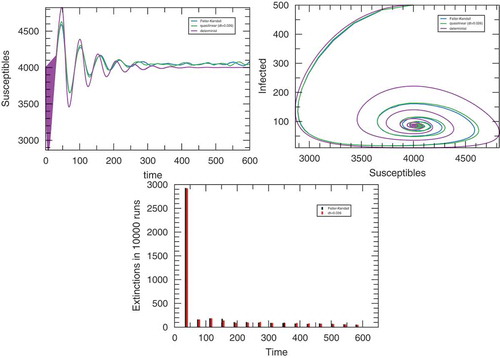
In Figure 1, it is shown that the approximated method closely follows the exact simulation in contrast with the deterministic method that presents large departures after reaching the minimum number of infected individuals (upper right panel in the figure). Both the total number of runs (out of ${10}^4$) where the infected population goes into extinction and the distribution in time of these events is well represented by the approximation method (no extinction is possible in the deterministic simulation).

Figure 1. Simulation outputs of the SIRS model for $S_0=6000,rr=0.8,ri=0.0002,rs=0.02$ and $dt=0.02$ for the approximated stochastic simulation. The upper left panel displays the average time-trace of the number of infected individuals. Upper right: average trace of the trajectory in the $(S,I)$ plane. The bottom panel displays the number of process in which the infected population became extinct. In all cases, ${10}^4$simulations where performed.

6. Concluding remarks

The goal of this manuscript has been to discuss, develop and implement a quasilinear approximation to the Feller–Kendall algorithm for Markov Jump processes. The work follows closely the ideas in Solari and Natiello (2014), where linear and constant transition rates are discussed. In the present work, we extend those ideas to the more useful situation where rates are not necessarily linear and – quite important – they are also time-dependent. The relevance of the use of approximations ultimately lies in the judgement of the user. However, for population problems with realistic aspirations, the Feller–Kendall algorithm soon becomes too slow and reliable approximations are a reasonable way out. The alternatives available for choosing a proper approximation level are therefore also discussed.

Acknowledgements

M.A.N. acknowledges support from the Kungliga Fysiografiska Sällskapet (Lund, Sweden). R.B., M.O. and H.G.S. acknowledge support from Buenos Aires University under grant 20020130100361BA.

Additional information

Funding

This work was supported by the Kungliga Fysiografiska Sällskapet i Lund [--]; Universidad de Buenos Aires [20020130100361BA].

Notes on contributors

Mario A. Natiello

The authors participate in several long-term collaborations concerning the propagation of epidemic diseases in different populations (ranging from human groups to crops) with emphasis in those propagated by vectors, thus involving ecological aspects. The aim of this cross-disciplinary group is to develop the understanding of general population dynamics problems combining mathematical and biological expertise in a way that goes beyond the individual disciplines.

Appendix A.

Properties of exact solutions

We may think of $\mathrm{\Phi }$ as the conditional probability of the standard formulation of the Kolmogorov Forward Equation. ${\mathbf{X}}^0$ resumes all the information of the path at time $s$ that is relevant for the future (the condition), while $\mathbf{n}$ represents the number of events that have occurred after the initial time $s$. Thus, $\mathrm{\Phi }=\mathrm{\Phi }(\mathbf{z},t;{\mathbf{X}}^0,s)$. The transition probabilities may then show a dependence with time as well. To lighten the notation, we have suppressed the initial time in the arguments since we will seldom use it.

The description by events offers more information than the description by states of the population. The projection of the increments in the number of events, $\mathbf{n}$, onto population states is made by the matrix $\delta$ with elements ${\delta }_j^{\alpha }$ which in general is an integer-valued rectangular matrix of dimensions $(E\times N)$ with $E\ge N$. Since the matrix is rectangular, we are certain to have zero eigenvalues whenever $E>N$. We call the associated eigenvectors, ${\mathbf{v}}_j$, structural zeros. We take the following results from (Solari & Natiello, 2014):

Definition. A nonzero vector ${\mathbf{v}}_j$ such that ${\sum }_{\alpha }{\delta }_j^{\alpha }{v}_k^{\alpha }=0$, for $j=1,\cdots ,N$ is called a structural zero of $\delta$.

There are $E-N$ structural zeros. The basis of the space of events can be taken as the union of the $N$ vectors ${\mathbf{x}}_j$ with components $x_j^{\alpha }={\delta }_j^{\alpha }$ and the $E-N$ vectors ${\mathbf{v}}_j$. We have that ${\mathbf{x}}_j\cdot {\mathbf{v}}_{\mathbf{k}}=0$.

Equation (1) can be formally written as:

$\frac{\mathrm{\partial }\mathrm{\Phi }}{\mathrm{\partial }t}\equiv \mathcal{L}({\mathbf{X}}^0,t)\mathrm{\Phi }(\mathbf{z},t;{\mathbf{X}}^0,s)=\sum _{\mathbf{n}}{\mathbf{z}}^{\mathbf{n}}\sum _{\alpha }(z_{\alpha }-1)W_{\alpha }(\mathbf{X}(\mathbf{n}))P(\mathbf{n},t,{\mathbf{X}}^0).$

Thus the operator $\mathcal{L}$ is defined as acting over the monomials ${\mathbf{z}}^{\mathbf{n}}$as $\mathcal{L}({\mathbf{X}}^0,s){\mathbf{z}}^{\mathbf{n}}={\mathbf{z}}^{\mathbf{n}}\sum _{\alpha }(z_{\alpha }-1)W_{\alpha }({\mathbf{X}}^0+\delta \mathbf{n})$. If we write $\mathbf{X}(\mathbf{n})={\mathbf{X}}^0+\delta \mathbf{n}$ it is clear that

$\mathcal{L}({\mathbf{X}}^0,s){\mathbf{z}}^{\mathbf{n}+\mathbf{k}}={\mathbf{z}}^{\mathbf{k}}\mathcal{L}({\mathbf{X}}^0+\delta \mathbf{k},s){\mathbf{z}}^{\mathbf{n}}$

and then

(A1) $\frac{\mathrm{\partial }({\mathbf{z}}^{\mathbf{k}}\mathrm{\Phi })}{\mathrm{\partial }t}\equiv \mathcal{L}({\mathbf{X}}^0,t){\mathbf{z}}^{\mathbf{k}}\mathrm{\Phi }(\mathbf{z},t;{\mathbf{X}}^0,t)={\mathbf{z}}^{\mathbf{k}}\mathcal{L}({\mathbf{X}}^0+\delta \mathbf{k},t)\mathrm{\Phi }(\mathbf{z},t;{\mathbf{X}}^0,s)).$(A1)

We call $K(\mathbf{z},t;{\mathbf{X}}^0,s)$ the operator that solves the Kolmogorov Backward Equation

(A2) $\frac{\mathrm{\partial }K(\mathbf{z},t;{\mathbf{X}}^0,s)}{\mathrm{\partial }s}=-K(\mathbf{z},t;{\mathbf{X}}^0,s)\mathcal{L}({\mathbf{X}}^0,s),$(A2)

with $K(\mathbf{z},t;{\mathbf{X}}^0,t)\mathbf{1}=\mathrm{\Phi }(\mathbf{z},t;{\mathbf{X}}^0,t)$, where $\mathbf{1}$ is the generating function corresponding to no events. Following (Solari & Natiello, 2003), we have

$\mathrm{\Phi }=\psi +\mathrm{\Delta },$

where $\mathrm{\Delta }(\mathbf{z},s;{\mathbf{X}}^0,s)=0$ and then we can write

$\mathrm{\Delta }(\mathbf{z},t;{\mathbf{X}}^0,s)=-{\int }_s^t\frac{d}{d{s}^{\mathrm{\prime }}}\left(K(\mathbf{z},t;{\mathbf{X}}^0,s^{\mathrm{\prime }})\psi (\mathbf{z},s^{\mathrm{\prime }};{\mathbf{X}}^0,s)\right)d{s}^{\mathrm{\prime }}.$

Thus, we obtain

$\begin{array}{c}\mathrm{\Delta }(\mathbf{z},t;{\mathbf{X}}^0,s)=-\left(K(\mathbf{z},t;{\mathbf{X}}^0,s^{\mathrm{\prime }})\psi (\mathbf{z},s^{\mathrm{\prime }};{\mathbf{X}}^0,s)\right){|}_s^t\\ =-\mathbf{I}\mathbf{d}\psi (\mathbf{z},t;{\mathbf{X}}^0,s)+K(\mathbf{z},t;{\mathbf{X}}^0,s)\mathbf{1}\\ =\mathrm{\Phi }-\psi .\end{array}$

where $Id$ is the identity operator. Then,

(A3) $\mathrm{\Delta }(\mathbf{z},t;{\mathbf{X}}^0,s)={\int }_s^t\left(K(\mathbf{z},t;{\mathbf{X}}^0,s^{\mathrm{\prime }})\left(\mathcal{L}({\mathbf{X}}^0,s^{\mathrm{\prime }})-\frac{d}{d{s}^{\prime }}\right)\psi (\mathbf{z},s^{\mathrm{\prime }};{\mathbf{X}}^0,s)\right)d{s}^{\mathrm{\prime }}.$(A3)

Recalling Equation (8)

$(\mathcal{L}({\mathbf{X}}^0,s^{\mathrm{\prime }})-\frac{d}{d{s}^{\mathrm{\prime }}})\psi (\mathbf{z},s^{\mathrm{\prime }};{\mathbf{X}}^0,s)=\sum _{\mathbf{n}}{\mathbf{z}}^{\mathbf{n}}\sum _k\sum _{\alpha \in B_k}(z_{\alpha }-1)\left((f_{\alpha }(\mathbf{X})-r_{\alpha }^k)\right)X_k\bar{P}(\mathbf{n},s^{\mathrm{\prime }},{\mathbf{X}}^0,s)$

where $\bar{P}$ are the approximated probabilities,

$\psi (\mathbf{z},t;{\mathbf{X}}^0,s)=\sum _{\left\{\mathbf{n}\right\}}{\mathbf{z}}^{\mathbf{n}}\bar{P}(\mathbf{n},t,{\mathbf{X}}^0,s).$

Using the later and Equation (A1), we obtain the result

$\begin{array}{c}\mathrm{\Delta }(z,t;{\mathbf{X}}^0,s)\\ ={\int }_0^t\left(\sum _{k,\alpha \in B_k,\left\{n\right\}}{z}^{\mathbf{n}}\bar{P}(n,s^{\mathrm{\prime }};{\mathbf{X}}^0,s)\left(\left(f_{\alpha }(\mathbf{X})-r_{\alpha }^k\right)X_k\right)\left(z_{\alpha }\mathrm{\Phi }(z,t;\mathbf{X}+{\delta }_{\alpha },s^{\mathrm{\prime }})-\mathrm{\Phi }(z,t;\mathbf{X},s^{\mathrm{\prime }})\right)\right)d{s}^{\mathrm{\prime }}.\end{array}$

A.1. The approximation lemma

The form of the approximations to the generating function can also be obtained by the following iterative scheme starting from Equation (12), recalling also the auxiliary definition in Equation (11):

(A4) $\begin{array}{c}{w}_k^{(n+1)}(\mathbf{z},t,t-t_0)=H_k(t,t_0,0)\\ +{\int }_0^{t-t_0}{H}_k(t,t_0,\tau )\sum _{\beta \in B_k}{r}_{\beta }^k(t-\tau )z_{\beta }{\left[\prod _{j\ne k}{\left(w_j(z,t,\tau )\right)}^{{\delta }_j^{\beta }}\right]}^{(n)}d\tau \end{array}$(A4)

with $w_k^{(0)}(\mathbf{z},t,t-t_0)=1$. The following Lemma was originally proved in (Solari & Natiello, 2014; Lemma 22). We add to the present version one more item (item e) and a slightly improved iteration scheme.

Lemma 5. For $t\in [0,h]$, $h=t-t_0>0$ sufficiently small and for each order of approximation $n\ge 0$, $w_k^{(n)}(\mathbf{z},t,t-t_0)$ in 12 is a polynomial generating function for one individual of the population, i.e., it has the following properties:

1. $w_k^{(n)}(z_1,\cdots ,z_E,t,t-t_0)$ is a polynomial of degree $n$ in $z_1,\cdots ,z_E$, where the coefficient of $z_1^{n_1},\cdots ,z_E^{n_E}$ is $O(h^p)$, with $p=n_1+\cdots +n_E$.

2. $w_k^{(n)}(1,\cdots ,1,t,t-t_0)=1$.

3. ${\mathrm{\Delta }}_k^{(n)}(\mathbf{z},t,h)=w_k^{(n)}(\mathbf{z},t,h)-w_k^{(n-1)}(\mathbf{z},t,h)=O(h^n)$, for $n\ge 1$.

4. The coefficients of $w_k^{(n)}(z_1,\cdots ,z_E,t,t-t_0)$ regarded as a polynomial in $\left\{z_{\alpha }\right\}$ are non-negative functions of time.

5. ${\mathrm{\Delta }}_k^n(\mathbf{z},t,h)\propto z^{(n-1)}(z-1)$, for $n\ge 1$.

Proof. We proceed inductively. For $n=0$, we set $w_k^{(0)}=1$ and replacing in the iterated form we obtain

$\begin{array}{rl}& w_k^1(\mathbf{z},t,t-t_0)=exp\left(-{\int }_0^{t-t_0}\sum _{\beta \in B_k}{r}_{\beta }^k(t-u)du\right)\\ & +{\int }_0^{t-t_0}exp\left(-{\int }_{\tau }^{t-t_0}\sum _{\beta \in B_k}{r}_{\beta }^k(t-u)du\right)\left(\sum _{\beta \in B_k}{r}_{\beta }^k(t-\tau )z_{\beta }\right)d\tau .\end{array}$

Noting that

$\begin{array}{rl}& \underset{0}{\overset{t-t_0}{\int }}\left(\sum _{\beta \in B_k}{r}_{\beta }^k(t-\tau )\right)exp\left(-\underset{\tau }{\overset{t-t_0}{\int }}\sum _{\beta \in B_k}{r}_{\beta }^k(t-u)du\right)d\tau \\ & =\underset{0}{\overset{t-t_0}{\int }}\frac{d}{d\tau }\left(exp\left(-\underset{\tau }{\overset{t-t_0}{\int }}\sum _{\beta \in B_k}{r}_{\beta }^k(t-u)du\right.\right)d\tau \\ & =1-exp\left(-\underset{0}{\overset{t-t_0}{\int }}\sum _{\beta \in B_k}{r}_{\beta }^k(t-\tau )d\tau \right),\end{array}$

we realise that properties (a)–(e) hold for $n=1$. In particular,

${\mathrm{\Delta }}_k^1(\mathbf{z},t,h)={\int }_0^{h}exp\left(-{\int }_{\tau }^h\sum _{\beta \in B_k}{r}_{\beta }^k(t-u)du\right)\left(\sum _{\beta \in B_k}{r}_{\beta }^k(t-\tau )(z_{\beta }-1)\right)d\tau .$

Under the iterative scheme A4, assuming that the properties hold for arbitrary $n-1$ (with $n\ge 2$), it is immediate that property (a) holds also for $n$, since the iterative scheme adds one power of $z$ to the previous polynomial. Moreover, the correction ${\mathrm{\Delta }}_k^{(n)}(\mathbf{z},t,h)=w_k^{(n)}(\mathbf{z},t,h)-w_k^{(n-1)}(\mathbf{z},t,h)$ reads (with the auxiliary $H_k$ defined in Equation 11):

$\begin{array}{c}{\mathrm{\Delta }}_k^{(n)}(\mathbf{z},t,h)={\int }_0^h{H}_k(t,t-h,\tau )\left(\sum _{\beta \in B_k}\left(r_{\beta }^k(t-\tau )z_{\beta }{\left[\prod _{j\ne k}{\left(w_j(z,t,\tau )\right)}^{{\delta }_j^{\beta }}\right]}^{(n-1)}\right)\right)d\tau \\ -{\int }_0^h{H}_k(t,t-h,\tau )\left(\sum _{\beta \in B_k}\left(r_{\beta }^k(t-\tau )z_{\beta }{\left[\prod _{j\ne k}{\left(w_j(z,t,\tau )\right)}^{{\delta }_j^{\beta }}\right]}^{(n-2)}\right)\right)d\tau .\end{array}$

Note that throughout, we will consider the individual $w$’s inside each square bracket to be truncated to the same order of the bracket, since this implies no loss of generality. Thus, property (b) follows since by the inductive hypothesis $w_j^{(n-1)}(1,t,t-t_0)=1$ and hence ${\mathrm{\Delta }}_k^{(n)}(1,t,h)=0$. Using that

${\left[w_j^{\delta {}_j^{\beta }}\right]}^{(n-1)}={\left[w_j^{\delta {}_j^{\beta }}\right]}^{(n-2)}+\delta {}_j^{\beta }{\left[w_j^{\delta {}_j^{\beta }-1}\right]}^{(n-2)}{\mathrm{\Delta }}_k^{(n-1)}+O(t^{2n-2})$

and that ${\mathrm{\Delta }}_k^{(n)}=O(t^n)$ for $n\ge 2$, we can drop the higher order terms. Thus, we have (for arbitrary $n>1$),

$\begin{array}{c}{\mathrm{\Delta }}_k^{(n)}(\mathbf{z},t,h)={\int }_0^h{H}_k(t,t-h,\tau )\sum _{\beta \in B_k}\left(r_{\beta }^k(t-\tau )z_{\beta }\sum _{j\ne k}\left({\delta }_j^{\beta }{\left[w_j^{{\delta }_j^{\beta }-1}\right]}^{(n-2)}{\mathrm{\Delta }}_j^{(n-1)}\right)\right)d\tau \\ +O(t^{2n-1}),\end{array}$

but since ${\mathrm{\Delta }}_k^{(n-1)}=O(t^{n-1})$ we can also drop higher order terms in $w_j^{(n-2)}=1+O(t)$ since they do not contribute to the leading order. Finally,

$\begin{array}{c}{\mathrm{\Delta }}_k^{(n)}(\mathbf{z},t,h)={\int }_0^h{H}_k(t,t-h,\tau )\sum _{\beta \in B_k}\left(r_{\beta }^k(t-\tau )z_{\beta }\sum _{j\ne k}\left({\delta }_j^{\beta }{\mathrm{\Delta }}_k^{(n-1)}\right)\right)d\tau \\ +O(t^{n+1}),\end{array}$

thus giving both (c) and (e). For (d) we observe that,

$\begin{array}{c}{w}_k^{(n)}(\mathbf{z},t,t-t_0)=w_k^{(1)}(\mathbf{z},t,t-t_0)+\sum _{m=2}^n{\mathrm{\Delta }}_k^{(m)}(\mathbf{z},t,t-t_0)\\ =1+\sum _{m=1}^n{\mathrm{\Delta }}_k^{(m)}(\mathbf{z},t,t-t_0).\end{array}$

Inserting the expression for ${\mathrm{\Delta }}_k^{(n)}(\mathbf{z},t)$ above, we may write:

$\begin{array}{c}{w}_k^{(n)}(\mathbf{z},t,t-t_0)=w_k^{(1)}(\mathbf{z},t,t-t_0)\\ +{\int }_0^{t-t_0}{H}_k(t,t_0,\tau )\sum _{\beta \in B_k}{r}_{\beta }^k(t-\tau )z_{\beta }\left({\left[\prod _{j\ne k}{\left(w_j(z,t,\tau )\right)}^{{\delta }_j^{\beta }}\right]}^{(n-1)}-1\right)d\tau .\end{array}$

Recalling the expression for $w^{(1)},$ we finally obtain:

$\begin{array}{c}{w}_k^{(n)}(z,t,t-t_0)=H_k(t,t_0,0)\\ +{\int }_0^{t-t_0}{H}_k(t,t_0,\tau )\sum _{\beta \in B_k}{r}_{\beta }^k(t-\tau )z_{\beta }{\left[\prod _{j\ne k}{\left(w_j(z,t,\tau )\right)}^{{\delta }_j^{\beta }}\right]}^{(n-1)}d\tau .\end{array}$

Hence, if $w_k^{(n-1)}$ is a polynomial with positive coefficients, the same property holds for $w_k^{(n)}$since it results from multiplication by positive numbers and integration term by term.

It remains to be shown that A4 converges towards a solution of 12, or what is the same, that $\underset{n\to \mathrm{\infty }}{lim}\left|w_k(z)-w_k^{(n)}(z)\right|=0$. However, for $m>0$,

$\left|w_k^{(n+m)}-w_k^{(n)}\left|\le \sum _{j=0}^{m-1}\right|w_k^{(n+j+1)}-w_k^{(n+j)}\left|\le C\right|z^{n+1}(z-1)\right||t{|}^{n+1}$

with

$C=\underset{0\le \tau \le t-t_0}{sup}\left(exp(-{\int }_{\tau }^{t-t_0}\sum _{\beta \in B_k}{r}_{\beta }^k(t-u)du)\sum _{\beta \in B_k}{r}_{\beta }^k(t-\tau )\right).$

Then, for bounded transition rates and sufficiently small $t$, the iterative scheme is a contraction map and by Banach’s theorem has a fixed point which is the solution we are looking for.

References

- Aparicio, J. P., Natiello, M., & Solari, H. G. (2012). The quasi-deterministic limit of population dynamics. International Journal of Applied Mathematics and Statistics, 26(2), 30–45.
- Durrett, R. (2001). Essentials of stochastic processes. New York: Springer Verlag.
- Ethier, S. N., & Kurtz, T. G. (1986). Markov processes. New York: John Wiley and Sons.
- Feller, W. (1949). On the theory of stochastic processes, with particular reference to applications (pp. 403–432). University of California Press.
- Feller, W. (1940). On the integro-differential equations of purely discontinuous Markoff processes. Transactions of the American Mathematical Society, 480(3), 488–515. ISSN 00029947. Retrieved from http://www.jstor.org/stable/1990095
- Fernández, M. L., Otero, M., Schweigmann, N., & Solari, H. G. (2013). A mathematically assisted reconstruction of the initial focus of the yellow fever outbreak in buenos aires (1871). Papers in Physics, 5, 50002. doi:10.4279/PIP.050002
- Kendall, D. G. (1949). Stochastic processes and population growth. Journal of the Royal Statistical Society. Series B (Methodological), 11, 230–282. doi:10.1111/j.2517-6161.1949.tb00032.x
- Kendall, D. G. (1950). An artificial realization of a simple “birth-and-death” process. Journal of the Royal Statistical Society. Series B (Methodological), 12, 116–119. doi:10.1111/j.2517-6161.1950.tb00048.x
- Kolmogoroff, A. (1931). Über die analytischen methoden in der wahrscheinlichkeitsrechnung. Mathematische Annalen, 104, 415–458. ISSN 0025–5831. doi:10.1007/BF01457949
- Malthus, T. 1798. An essay on the principle of population. www.esp.org. London: Electronic Scholarly Publishing Project. Retrieved from http://www.esp.org/books/malthus/population/malthus.pdf
- McKendrick, A. G. (1914). Studies on the theory of continuous probabilities, with special reference to its bearing on natural phenomena of a progressive nature. Proceedings of the London Mathematical Society, s2–13, 401–416. doi:10.1112/plms/s2-13.1.401
- Otero, M., Solari, H. G., & Schweigmann, N. (2006). A stochastic population dynamic model for Aedes aegypti: Formulation and application to a city with temperate climate. Bulletin of Mathematical Biology, 68, 1945–1974. doi:10.1007/s11538-006-9067-y
- Solari, H. G., & Natiello, M. A. (2003). Stochastic population dynamics: The Poisson approximation. Physical Review E, 67, 31918. doi:10.1103/PhysRevE.67.031918
- Solari, H. G., & Natiello, M. A. (2014). Linear processes in stochastic population dynamics: Theory and application to insect development. The Scientific World Journal - Journal of Probability and Statistics, 2014, ID 873624, 1–15. Retrieved from http://downloads.hindawi.com/journals/tswj/aip/873624.pdf
- Zanotti, G., De Majo, M., Sol, I. A., Nicolás, S., Campos, R. E., & Fischer, S. (2015). New records of Aedes aegypti at the southern limit of its distribution in Buenos Aires Province, Argentina. Journal of Vector Ecology, 400(2), 408–411. doi:10.1111/jvec.12181