The Gompertz Fréchet distribution: Properties and applications

Abstract

In this paper, a new compound continuous distribution named the Gompertz Fréchet distribution which extends the Frèchet distribution was developed. Its various statistical properties were also derived and estimation of model parameters was considered using the maximum likelihood estimation method. The application of the Gompertz Fréchet distribution was provided using real-life data sets and its performance was compared with Gompertz Weibull distribution, Gompertz Lomax distribution and Gompertz Burr XII distribution.

Keywords:

• estimation
• Fréchet distribution
• generalization
• generalized models
• Gompertz family of distribution
• mathematical statistics
• statistical properties

PUBLIC INTEREST STATEMENT

Standard probability models have been found to be of immense importance in modeling real-life events; extending these distributions usually give rise to more suitable models that can withstand strong asymmetry. The four-parameter probability model that was proposed in this research is basically an extension of the Frechet distribution. Two additional parameters from the Gompertz family of distributions were introduced to the existing two parameters of the Frectchet distribution to produce a more flexible model. As a result of this, the Gompertz Fretchet distribution appears better than the Gompertz Weibull, Gompertz Burr XII and Gompertz Lomax distributions when applied to two real-life datasets.

1. Introduction

Fréchet distribution was developed by Maurice Fréchet in 1927. It is a continuous probability distribution and can also be called the Inverse Weibull distribution. The Inverse Rayleigh and Inverse Exponential distributions can be considered as special cases of the Fréchet distribution. Fréchet distribution has several applications; some of which can be found in hydrology and finance for modeling extreme events. Some further details about the Fréchet distribution including its applications are available in Harlow (2002), Morales (2005), Nadarajah and Kotz (2008), Zaharim, Najid, Razali, and Sopian (2009), Mubarak (2011), and Pehlivan and Vuong (2011). The cumulative distribution function (cdf) and probability density function of the Fréchet distribution (Fr) are:

(1) $G(x,\alpha ,\beta )=exp\left[-{\left(\frac{\alpha }{x}\right)}^{\beta }\right]$(1)

and

(2) $g(x,\alpha ,\beta )=\beta {\alpha }^{\beta }{x}^{-\beta -1}exp\left[-{\left(\frac{\alpha }{x}\right)}^{\beta }\right]$(2)

respectively, where $\alpha >0$ and $\beta >0$ are scale and shape parameters, respectively.

Some extensions of the Fréchet distribution have previously been proposed in the literature, the Beta Fréchet Distribution (Barreto-Souza, Cordeiro, & Simas, 2011), Weibull Fréchet distribution (Afify, Yousof, Cordeiro, Ortega, & Nofal, 2016) and the Logistic Fréchet distribution (Tahir, Cordeiro, Alzaatreh, Mansoor, & Zubair, 2016) are remarkable examples. This paper is however interested in extending the Fréchet distribution using the Gompertz family of distribution proposed by Alizadeh, Cordeiro, Pinho, and Ghosh (2017). One of the motivations of this study is the ability of the Gompertz family of distribution to perform creditably well than other well-known families of distributions as noted by Oguntunde, Khaleel, Ahmed, Adejumo, and Odetunmibi (2017) where the superiority of the Gompertz Lomax distribution over the Weibull Lomax, Beta Lomax and Kumaraswamy Lomax distributions was demonstrated.

It is worthy of note that other generalized families of distributions exist in the literature, examples of which include the Beta generalized family of distribution and many others which are listed in Merovci, Khaleel, Ibrahim, and Shitan (2016), Oguntunde, Adejumo, Okagbue, and Rastogi (2016), Oguntunde et al. (2018) and several other authors but the Gompertz family of distribution is well preferred in this research because it has not been widely explored despite its potentials. This research is aimed at extending the Fréchet distribution in order to increase its potentials in modeling extreme events both in reliability studies, hydrology, finance and so on.

The densities of the Gompertz Fréchet distribution are derived in Section 2 of this paper, its various statistical properties are established in Section 3 while applications to real-life data sets are provided in Section 4. The potentials of the proposed Gompertz Fréchet distribution would be demonstrated with respect to the Gompertz Lomax, Gompertz Weibull and Gompertz Burr XII distributions.

2. The Gompertz Fréchet (GoFr) distribution

The densities of the Gompertz generalized family of distribution are:

(3) $F(x)=1-e^{\left(\frac{\theta }{\gamma }\right)\left\{1-{\left[1-G(x)\right]}^{-\gamma }\right\}}$(3)

and

(4) $f(x)=\theta g(x){\left[1-G(x)\right]}^{-\gamma -1}{e}^{\left(\frac{\theta }{\gamma }\right)\left\{1-{\left[1-G(x)\right]}^{-\gamma }\right\}}$(4)

where $\theta$ and $\gamma$ are extra shape parameters, $F(x)$ and $f(x)$ are the cdf and pdf, respectively. These shape parameters are to introduce/induce skewness into the parent distribution and this, however, increased the ability of the proposed model in modeling real events.

Therefore, the cdf of the GoFr distribution is obtained by substituting the expression in Equation (1) into Equation (3) as follows:

(5) $F(x,\alpha ,\beta ,\gamma ,\theta )=1-exp\left[\frac{\theta }{\gamma }\left(1-{\left\{1-exp\left[-{\left(\frac{\alpha }{x}\right)}^{\beta }\right]\right\}}^{-\gamma }\right)\right]$(5)

The corresponding pdf of the GoFr is given by:

(6) $\begin{array}{rl}& f(x,\alpha ,\beta ,\gamma ,\theta )=\theta \beta {\alpha }^{\beta }{x}^{-\beta -1}exp\left[-{\left(\frac{\alpha }{x}\right)}^{\beta }\right]{\left\{exp\left[-{\left(\frac{\alpha }{x}\right)}^{\beta }\right]\right\}}^{-\gamma -1}\\ & \ast exp\left[\frac{\theta }{\gamma }\left(1-{\left\{1-exp\left[-{\left(\frac{\alpha }{x}\right)}^{\beta }\right]\right\}}^{-\gamma }\right)\right]\end{array}$(6)

where $\alpha >0$ is the scale parameter, $\beta >0$, $\gamma >0$ and $\theta >0$ are shape parameters, respectively.

Plots for the GoFr distribution at various parameter values are as shown in Figure 1:

Figure 1. PDF of the Gomp_ertz Frechet distribution.

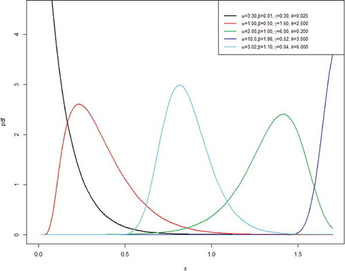
Obviously, the plots in Figure 1 reveal the shape of the GoFr distribution as being unimodal, increasing or decreasing.

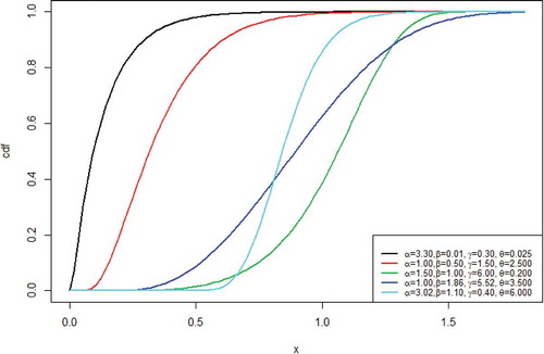
Possible plots for the cdf of the GoFr distribution are as shown in Figure 2:

Figure 2. CDF of the Gompertz Frechet distribution.

2.1. Expansions for the distribution and density functions

Expansions for the cdf and pdf of the GoFr distribution are provided as:

(7) $\begin{array}{rl}& F(x,\alpha ,\beta ,\gamma ,\theta )=1-\sum _{i=0}^{\mathrm{\infty }}\sum _{j=0}^i\sum _{k=0}^{\mathrm{\infty }}\frac{{(-1)}^{i+k}}{i!k!}{\left(\frac{\theta }{\gamma }\right)}^i\left(\begin{array}{c}i\\ j\end{array}\right)\left(\begin{array}{c}-j\gamma \\ k\end{array}\right)\\ & \ast {\left\{exp\left[-{\left(\frac{\alpha }{x}\right)}^{\beta }\right]\right\}}^k\end{array}$(7)

and

(8) $\begin{array}{rl}& f(x,\alpha ,\beta ,\gamma ,\theta )=\beta {\alpha }^{\beta }{x}^{-\beta -1}\sum _{i=0}^{\mathrm{\infty }}\sum _{j=0}^i\sum _{k=0}^{\mathrm{\infty }}\frac{{(-1)}^{i+k}\theta {}^{i+1}}{{\gamma }^{i}i!k!}\left(\begin{array}{c}i\\ j\end{array}\right)\left(\begin{array}{c}-\gamma (j+1)-1\\ k\end{array}\right)\\ & \ast {\left\{exp\left[-{\left(\frac{\alpha }{x}\right)}^{\beta }\right]\right\}}^{k+1}\end{array}$(8)

respectively.

The expressions in Equations (7) and (8) can further be used to obtain the moments, moment generating function (mgf) and entropy of the GoFr distribution.

3. Statistical properties

Statistical properties like the quantile function, median, survival function, hazard function, reversed hazard function, odds function, distribution of order statistics and estimation of parameters are provided in this section.

3.1. Quantile function and median

The quantile function is the inverse of the cdf and it can be represented mathematically as:

$Q(u)=F^{-1}(u)$

Therefore, the quantile function of the GoFr distribution is derived as:

(9) $Q(u)=\alpha {\left[-log\left(1-{\left\{1-\left[\frac{\gamma }{\theta }log(1-u)\right]\right\}}^{\frac{-1}{\gamma }}\right)\right]}^{\frac{-1}{\beta }}$(9)

where $U\sim Uniform(0,1)$

The median for the GoFr distribution is obtained by substituting $u=0.5$ in Equation (9) as:

(10) $Median=\alpha {\left[-log\left(1-{\left\{1-\left[\frac{\gamma }{\theta }log(0.5)\right]\right\}}^{\frac{-1}{\gamma }}\right)\right]}^{\frac{-1}{\beta }}$(10)

Other quantiles can be obtained from Equation (9) when the appropriate value of $u$ is substituted.

3.2. Reliability analysis

Survival Function: The Survival (or reliability) function is derived as follows:

$S(x)=1-F(x)$

Therefore, the survival function of the GoFr distribution is given as:

(11) $S(x)=exp\left[\frac{\theta }{\gamma }\left(1-{\left\{1-exp\left[-{\left(\frac{\alpha }{x}\right)}^{\beta }\right]\right\}}^{-\gamma }\right)\right]$(11)

where $\alpha >0$, $\beta >0$, $\gamma >0$ and $\theta >0$.

Hazard Function: The hazard function which can also be called the failure rate is derived from:

$h(x)=\frac{f(x)}{S(x)}$

So, the hazard function of the GoFr distribution is:

(12) $h(x,\alpha ,\beta ,\gamma ,\theta )=\theta \beta {\alpha }^{\beta }{x}^{-\beta -1}exp\left[-{\left(\frac{\alpha }{x}\right)}^{\beta }\right]{\left\{exp\left[-{\left(\frac{\alpha }{x}\right)}^{\beta }\right]\right\}}^{-\gamma -1}$(12)

where $\alpha >0$, $\beta >0$, $\gamma >0$ and $\theta >0$.

Plots for the failure rate of the GoFr distribution are as shown in Figure 3:

Figure 3. Plots for the hazard function of Gompertz Frechet distribution.

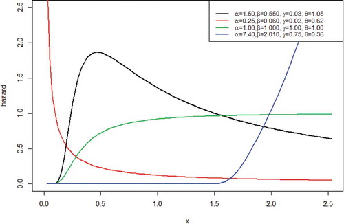
The plots in Figure 3 indicate that the shape of the failure rate of the GoFr distribution could be decreasing, increasing and unimodal. This implies that the GoFr distribution can be used to describe and model real-life phenomena whose failure rates are decreasing, increasing or inverted bathtub.

Reversed Hazard Function: The reversed hazard function is derived from:

$r(x)=\frac{f(x)}{F(x)}$

So, the expression for the reversed hazard function of the GoFr distribution is given as:

(13) $\begin{array}{rl}& r(x,\alpha ,\beta ,\gamma ,\theta )=\theta \beta {\alpha }^{\beta }{x}^{-\beta -1}exp\left[-{\left(\frac{\alpha }{x}\right)}^{\beta }\right]{\left\{exp\left[-{\left(\frac{\alpha }{x}\right)}^{\beta }\right]\right\}}^{-\gamma -1}\\ & \ast exp\left[\frac{\theta }{\gamma }\left(1-{\left\{1-exp\left[-{\left(\frac{\alpha }{x}\right)}^{\beta }\right]\right\}}^{-\gamma }\right)\right]\\ & \ast {\left[1-exp\left[\frac{\theta }{\gamma }\left(1-{\left\{1-exp\left[-{\left(\frac{\alpha }{x}\right)}^{\beta }\right]\right\}}^{-\gamma }\right)\right]\right]}^{-1}\end{array}$(13)

where $\alpha >0$, $\beta >0$, $\gamma >0$ and $\theta >0$.

Odds Function: The odds function is derived from:

$O(x)=\frac{F(x)}{S(x)}$

Therefore, the expression for the odds function of the GoFr distribution is given as:

(14) $r(x,\alpha ,\beta ,\gamma ,\theta )=\frac{1-exp\left[\frac{\theta }{\gamma }\left(1-{\left\{1-exp\left[-{\left(\frac{\alpha }{x}\right)}^{\beta }\right]\right\}}^{-\gamma }\right)\right]}{exp\left[\frac{\theta }{\gamma }\left(1-{\left\{1-exp\left[-{\left(\frac{\alpha }{x}\right)}^{\beta }\right]\right\}}^{-\gamma }\right)\right]}$(14)

where $\alpha >0$, $\beta >0$, $\gamma >0$ and $\theta >0$.

3.3. Order statistics

If $x_1,x_2,...,x_n$ denote random samples from the densities of a GoFr distribution as defined in (5) and Equation (6) respectively; the pdf of the $kth$ order statistics of the GoFr distribution is obtained as follows:

$f_{k:n}(x)=\frac{n!}{(k-1)!(n-1)!}f(x)[F(x){]}^{k-1}[1-F(x){]}^{n-k}$

Consequently, the pdf of $kth$ order statistics for the GoFr distribution is obtained as:

$f_{k:n}(x)=\frac{n!}{(k-1)!(n-1)!}\theta \beta {\alpha }^{\beta }{x}^{-\beta -1}exp\left[-{\left(\frac{\alpha }{x}\right)}^{\beta }\right]{\left\{exp\left[-{\left(\frac{\alpha }{x}\right)}^{\beta }\right]\right\}}^{-\gamma -1}$

$\ast exp\left[\frac{\theta }{\gamma }\left(1-{\left\{1-exp\left[-{\left(\frac{\alpha }{x}\right)}^{\beta }\right]\right\}}^{-\gamma }\right)\right]$

$\ast {\left[1-exp\left[\frac{\theta }{\gamma }\left(1-{\left\{1-exp\left[-{\left(\frac{\alpha }{x}\right)}^{\beta }\right]\right\}}^{-\gamma }\right)\right]\right]}^{k-1}$

(15) $\ast {\left[exp\left[\frac{\theta }{\gamma }\left(1-{\left\{1-exp\left[-{\left(\frac{\alpha }{x}\right)}^{\beta }\right]\right\}}^{-\gamma }\right)\right]\right]}^{n-k}$(15)

When $k=1$ the distribution of minimum order statistics for the GoFr distribution is therefore given as:

$f_{1:n}(x)=n\theta \beta {\alpha }^{\beta }{x}^{-\beta -1}exp\left[-{\left(\frac{\alpha }{x}\right)}^{\beta }\right]{\left\{exp\left[-{\left(\frac{\alpha }{x}\right)}^{\beta }\right]\right\}}^{-\gamma -1}$

(16) $\ast {\left[exp\left[\frac{\theta }{\gamma }\left(1-{\left\{1-exp\left[-{\left(\frac{\alpha }{x}\right)}^{\beta }\right]\right\}}^{-\gamma }\right)\right]\right]}^n$(16)

and when $k=n$ the distribution of maximum order statistics for the GoFr distribution is:

$f_{n:n}(x)=n\theta \beta {\alpha }^{\beta }{x}^{-\beta -1}exp\left[-{\left(\frac{\alpha }{x}\right)}^{\beta }\right]{\left\{exp\left[-{\left(\frac{\alpha }{x}\right)}^{\beta }\right]\right\}}^{-\gamma -1}$

$\ast exp\left[\frac{\theta }{\gamma }\left(1-{\left\{1-exp\left[-{\left(\frac{\alpha }{x}\right)}^{\beta }\right]\right\}}^{-\gamma }\right)\right]$

(17) $\ast {\left[1-exp\left[\frac{\theta }{\gamma }\left(1-{\left\{1-exp\left[-{\left(\frac{\alpha }{x}\right)}^{\beta }\right]\right\}}^{-\gamma }\right)\right]\right]}^{n-1}$(17)

3.4. Estimation of unknown parameter

The unknown parameters of the GoFr distribution are estimated using the maximum likelihood estimation (MLE) method as follows: let $x_1,x_2,...,x_n$ represent random samples which are distributed according to the pdf of the GoFr distribution, the likelihood function denoted by $l=f\left(x_i;\alpha ,\beta ,\gamma ,\theta \right)$ is derived from:

$l=\prod _{i=1}^n\left[f\left(x_1,x_2,...,x_n;\alpha ,\beta ,\gamma ,\theta \right)\right]$

Therefore, the log-likelihood function is:

$logl=nlog(\theta )+nlog(\beta )+\beta log(\alpha )-(\beta +1)\sum _{i=1}^{n}log(x_i)-\beta \sum _{i=1}^n\left(\frac{\alpha }{x_i}\right)$

(18) $+(\gamma +1)\beta \sum _{i=1}^n\left(\frac{\alpha }{x_i}\right)+\left(\frac{\theta }{\gamma }\right)\sum _{i=1}^n\left(1-{\left\{1-exp\left[-{\left(\frac{\alpha }{x_i}\right)}^{\beta }\right]\right\}}^{-\gamma }\right)$(18)

The solution of the non-linear equations of $\frac{dlogl}{d\alpha }=0$, $\frac{dlogl}{d\beta }=0$, $\frac{dlogl}{d\gamma }=0$ and $\frac{dlogl}{d\theta }=0$ results to the $ML$ estimates of parameters $\alpha ,\beta ,\gamma$ and $\theta$ respectively. The solution could not be obtained analytically except by numerical methods using software like R, MAPLE, SAS and so on.

4. Real life applications

For illustration purposes, the Gompertz Fréchet distribution was applied to two different real-life data sets and its performance was compared with the Gompertz Weibull, Gompertz Burr XII and Gompertz Lomax distributions. The criteria for selecting the distribution with the best fit are log-likelihood, Bayesian Information Criteria (BIC), Akaike Information Criteria (AIC), Hannan and Quinn Information Criteria (HQIC) and Consistent Akaike Information Criteria (CAIC). The value for the Shaphiro Wilks (W) test, Anderson Darling (A) statistic and Kolmogorov Smirnov (KS) statistic with its corresponding p-value are also provided. All the analyses in this study were performed using R software.

Data I: This data set relates to the strength of carbon fibers tested under tension at gauge lengths of 10 mm. The data has been recently reported and analyzed by Bi and Gui (2017) among others. The observations are as follows:

1.901, 2.132, 2.203, 2.228, 2.257, 2.350, 2.361, 2.396, 2.397, 2.445, 2.454, 2.474, 2.518, 2.522, 2.525, 2.532, 2.575, 2.614, 2.616, 2.618, 2.624, 2.659, 2.675, 2.738, 2.740, 2.856, 2.917, 2.928, 2.937, 2.937, 2.977, 2.996, 3.030, 3.125, 3.139, 3.145, 3.220, 3.223, 3.235, 3.243, 3.264, 3.272, 3.294, 3.332, 3.346, 3.377, 3.408, 3.435, 3.493, 3.501, 3.537, 3.554, 3.562, 3.628, 3.852, 3.871, 3.886, 3.971, 4.024, 4.027, 4.225, 4.395, 5.020

Table 1 shows the result of the analysis comparing the GoFr distribution to its counterpart distributions using DATA I:

Table 1. The ML estimates, $\mathit{l}$, $\mathit{A}IC$, $\mathit{C}AIC$, $\mathit{B}IC$ and $\mathit{H}QIC$ for the first data set

Model	ML Estim	l	AIC	CAIC	BIC	HQIC
GoW	$\hat{\alpha }$=0.7523	−59.5751	127.1502	127.8399	135.7227	130.5218
	$\hat{\beta }$=−0.1317
	$\hat{\gamma }$=0.3264
	$\hat{\theta }$=6.0883
GoBXII	$\hat{\alpha }$=0.0056	−62.3509	132.7019	133.3915	141.2744	136.0735
	$\hat{\beta }$=2.0355
	$\hat{\gamma }$=0.6809
	$\hat{\theta }$=3.5460
GoLom	$\hat{\alpha }$=0.0044	−64.9569	137.9139	138.6035	146.4864	141.2855
	$\hat{\beta }$=5.3157
	$\hat{\gamma }$=0.4533
	$\hat{\theta }$=1.4547
GoFr	$\hat{\alpha }$=0.6178	−55.8831	119.7662	120.4558	128.3387	123.1378
	$\hat{\beta }$=0.5458
	$\hat{\gamma }$=5.0302
	$\hat{\theta }$=2.6392

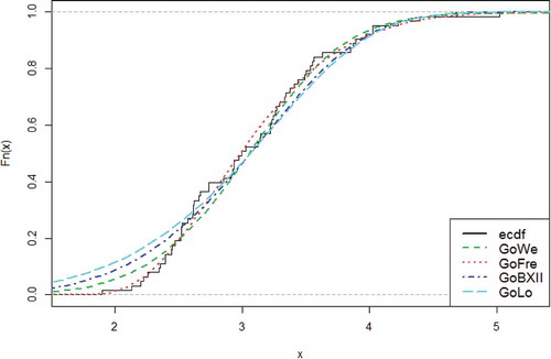
From Table 1, GoFr distribution has the highest log-likelihood value and lowest AIC, CAIC, BIC and HQIC values. Therefore, the GoFr is chosen as the model with the best fit among the distributions considered.

Table 2 shows the value for the W statistic, Anderson Darling statistic and the Kolmogorov Smirnov statistic for all the competing distributions using the first data set.

Table 2. The $\mathit{W}$, $\mathit{A}$, $\mathit{K}S$ and $\mathit{p}-value$ using the first data set

Model	$\mathit{W}$	$\mathit{A}$	$\mathit{K}S$	$\mathit{p}-value$
GoW	0.0945	0.6353	0.0913	0.6705
GoBXII	0.1275	0.8865	0.1012	0.5385
GoLom	0.1624	1.1128	0.1282	0.2515
GoFr	0.0433	0.2472	0.0687	0.9275

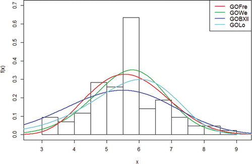
Figure 4 shows the histogram of the GoW, GoBXII, GoLom and GoFr distributions with respect to the first data set.

Figure 4. Histogram of the fitted distributions.

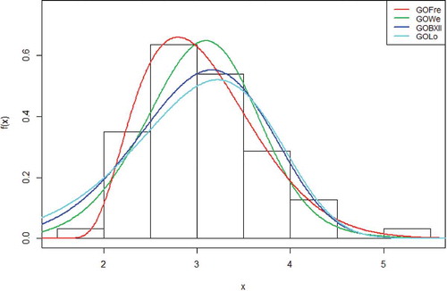
GoFr distribution represents the curve with the red line and it has been illustrated in Figure 4 to have the highest peak and however fits better to the histogram of the real data. The graph of the empirical cdfs of the GoW, GoBXII, GoLom and GoFr distributions with respect to the first data set is as shown in Figure 5:

Figure 5. Empirical cdf of the fitted distributions.

DATA II: This data set relates to civil engineering data with 85 hailing times. It has been previously used by Kotz and Dorp (2004). The observations are as follows:

4.79, 4.75, 5.40, 4.70, 6.50, 5.30, 6.00, 5.90, 4.80, 6.70, 6.00, 4.95, 7.90, 5.40, 3.50, 4.54, 6.90, 5.80, 5.40, 5.70, 8.00, 5.40, 5.60, 7.50, 7.00, 4.60, 3.20, 3.90, 5.90, 3.40, 5.20, 5.90, 4.40, 5.20, 7.40, 5.70, 6.00, 3.60, 6.20, 5.70, 5.80, 5.90, 6.00, 5.15, 6.00, 4.82, 5.90, 6.00, 7.30, 7.10, 4.73, 5.90, 3.60, 6.30, 7.00, 5.10, 6.00, 6.60, 4.40, 6.80, 5.60, 5.90, 5.90, 8.60, 6.00, 5.80, 5.40, 6.50, 4.80, 6.40, 4.15, 4.90, 6.50, 8.20, 7.00, 8.50, 5.90, 4.40, 5.80, 4.30, 5.10, 5.90, 4.70, 3.50, 6.80

Table 3 shows the result of the analysis with comparisons using DATA II:

Table 3. The ML estimates, $\mathit{l}$, $\mathit{A}IC$, $\mathit{C}AIC$, $\mathit{B}IC$ and $\mathit{H}QIC$ for the second data set

Model	ML Estim	$\mathit{l}$	$\mathit{A}IC$	$\mathit{C}AIC$	$\mathit{B}IC$	$\mathit{H}QIC$
GoW	$\hat{\alpha }$=0.4984	−133.559	275.1180	275.6180	284.8886	279.0480
	$\hat{\beta }$=−0.0826
	$\hat{\gamma }$=0.1869
	$\hat{\theta }$=6.1176
GoBXII	$\hat{\alpha }$=0.0020	−142.7397	293.4794	293.9794	303.2500	297.4094
	$\hat{\beta }$=1.8871
	$\hat{\gamma }$=0.9231
	$\hat{\theta }$=2.1938
GoLom	$\hat{\alpha }$=0.0050	−137.9373	283.8747	284.3747	293.6453	287.8047
	$\hat{\beta }$=6.7485
	$\hat{\gamma }$=0.1938
	$\hat{\theta }$=1.3562
GoFr	$\hat{\alpha }$=9.8016	−132.9584	273.9168	274.4168	283.6874	277.8468
	$\hat{\beta }$=3.8554
	$\hat{\gamma }$=1.6332
	$\hat{\theta }$=10.6159

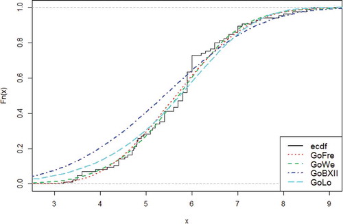
From Table 3, GoFr distribution has the highest log-likelihood value and lowest AIC, CAIC, BIC and HQIC values. Therefore, the GoFr is chosen as the model with the best fit among the distributions considered.

Table 4 shows the value for the W statistic, Anderson Darling statistic and the Kolmogorov Smirnov statistic for all the competing distributions using the second data set.

Table 4. The $\mathit{W}$, $\mathit{A}$, $\mathit{K}S$ and $\mathit{p}-value$ using the second data set

Model	$\mathit{W}$	$\mathit{A}$	$\mathit{K}S$	$\mathit{p}-value$
GoW	0.1045	0.5568	0.1261	0.1340
GoBXII	0.1223	0.6611	0.1754	0.0107
GoLom	0.2044	1.1845	0.1515	0.0404
GoFr	0.1284	0.1169	0.1961

Figure 6 shows the histogram of the GoW, GoBXII, GoLom and GoFr distributions using the second data set.

Figure 6. Histogram of the fitted distributions.

The graph of the empirical cdfs of the GoW, GoBXII, GoLom and GoFr distributions using the second data set is as shown in Figure 7.

Figure 7. Empirical cdf of the fitted distributions.

5. Conclusion

The Fréchet distribution has been successfully extended in this research. The densities of the Gompertz Fréchet distribution have been carefully derived and explicit expressions for its basic statistical properties have been established. The shape of the GoFr distribution could be increasing, decreasing or unimodal. It has also been established that the GoFr distribution exhibits increasing, decreasing and inverted bathtub (unimodal) failure rate. The Gompertz Fréchet distribution was applied to two real-life data sets and it was found to be better than the Gompertz Weibull, Gompertz Burr XII and Gompertz Lomax distributions based on the log-likelihood, AIC, CAIC, BIC and HQIC values posed by the distributions. It is concluded that the GoFr distribution is a good and competitive model for describing real-life phenomena. Further research would involve simulation studies using the quantile function obtained in this research.

Acknowledgements

The authors would like to appreciate Covenant University for providing an enabling environment for this study.

Additional information

Funding

The authors received no direct funding for this research.

Notes on contributors

Pelumi E. Oguntunde

Dr. Pelumi E. Oguntunde is a Statistician and a faculty in the Department of Mathematics, Covenant University, Nigeria. He has Bachelor of Science (B.Sc.) and Master of Science (M.Sc.) degrees in Statistics from University of Ilorin and University of Ibadan respectively. He earned his Ph.D. degree in Industrial Mathematics (Statistics Option) from Covenant University, Nigeria. His area of specialization is Mathematical Statistics. He teaches Statistics courses and he has made noticeable contributions to several scholarly journals especially in the area of probability distributions.

References

- Afify, A. Z., Yousof, H. M., Cordeiro, G. M., Ortega, E. M. M., & Nofal, Z. M. (2016). The Weibull Fréchet distribution and its applications. Journal of Applied Statistics, 43(14), 2608–12.
- Alizadeh, M., Cordeiro, G. M., Pinho, L. G. B., & Ghosh, I. (2017). The Gompertz-G family of distributions. Journal of Statistical Theory and Practice, 11(1), 179–207. doi:10.1080/15598608.2016.1267668
- Barreto-Souza, W., Cordeiro, G. M., & Simas, A. B. (2011). Some results for Beta Fréchet distribution. Communications in Statistics - Theory and Methods, 40(5), 798–811. doi:10.1080/03610920903366149
- Bi, Q., & Gui, W. (2017). Bayesian and classical estimation of stress-strength reliability for inverse Weibull lifetime models. Algorithms, 10, 71. doi:10.3390/a10020071
- Harlow, D. G. (2002). Applications of the Frechèt distribution function. International Journal of Material and Product Technology, 5(17), 482–495. doi:10.1504/IJMPT.2002.005472
- Kotz, S., & Dorp, J. R. (2004). Beyond beta: Other continuous families of distributions with bounded Support and applications (pp. 289). Singapore: World Scientific.
- Merovci, F., Khaleel, M. A., Ibrahim, N. A., & Shitan, M. (2016). The beta type X distribution: Properties with application. SpringerPlus, 5, 697. doi:10.1186/s40064-016-2271-9
- Morales, F. (2005). Estimation of Max-Stable Processes Using Monte Carlo Methods with Applications to Financial Risk Assessment. ( PhD dissertation). University of North Carolina, USA.
- Mubarak, M. (2011). Parameter estimation based on the Frechèt progressive type II censored data with binomial removals. International Journal of Quality, Statistics and Reliability, 2012. Article ID 245910.
- Nadarajah, S., & Kotz, S. (2008). Sociological models based on Frechèt random variables. Quality and Quantity, 42, 89–95. doi:10.1007/s11135-006-9039-1
- Oguntunde, P. E., Adejumo, A. O., Okagbue, H. I., & Rastogi, M. K. (2016). Statistical properties and applications of a new Lindley exponential distribution. Gazi University Journal of Science, 29(4), 831–838.
- Oguntunde, P. E., Khaleel, M. A., Adejumo, A. O., Okagbue, H. I., Opanuga, A. A., & Owolabi, F. O. (2018). The Gompertz Inverse Exponential (GoIE) distribution with Applications. Cogent Mathematics and Statistics, 5(1), 1507122. doi:10.1080/25742558.2018.1507122
- Oguntunde, P. E., Khaleel, M. A., Ahmed, M. T., Adejumo, A. O., & Odetunmibi, O. A. 2017. A new generalization of the lomax distribution with increasing, decreasing and constant failure rate. Modelling and Simulation in Engineering, 2017, Article ID 60431696. doi:10.1155/2017/6043169.
- Pehlivan, A., & Vuong, Q. (2011). International trade and supply function competition. Working paper. Turkey: Department of Economics, Bilkent University.
- Tahir, M. H., Cordeiro, G. M., Alzaatreh, A., Mansoor, M., & Zubair, M. (2016). The logistic-X family of distributions and its applications. Communications in Statistics-Theory and Methods, 45(24), 7326–7349. doi:10.1080/03610926.2014.980516
- Zaharim, A., Najid, S. K., Razali, A. M., & Sopian, K. (2009, February 24–26). Analyzing Malaysian wind speed data using statistical distribution. Proceedings of the 4th IASME/WSEAS International conference on Energy and Environment, University of Cambridge, United Kingdom.