On bounding the Thompson metric by Schatten norms

Abstract

The Thompson metric provides key geometric insights in the study of non-linear matrix equations and in many optimization problems. However, knowing that an approximate solution is within $d_T$ units, in the Thompson metric, of the actual solution provides little insight into how good the approximation is as a matrix or vector approximation. That is, bounding the Thompson metric between an approximate and accurate solution to a problem does not provide obvious bounds either for the spectral or the Frobenius norm, both Schatten norms, of the difference between the approximation and accurate solution. This paper reports such an upper bound, namely that $\parallel X-Y{\parallel }_p\le 2^{\frac{1}{p}}\frac{\left(e^d-1\right)}{e^d}max\left[\parallel X{\parallel }_p,\parallel Y{\parallel }_p\right]$ where ${∥\cdot ∥}_p$denotes the Schatten p-norm and $d$ denotes the Thompson metric between $X$ and $Y$. Furthermore, a more geometric proof leads to a slightly better bound in the case of the Frobenius norm, $\parallel X-Y{\parallel }_2\le \frac{\left(e^d-1\right)}{\sqrt{e^{2d}+1}}\sqrt{\parallel X{{\parallel }_2}^2+\parallel Y{{\parallel }_2}^2}\le 2^{\frac{1}{2}}\frac{\left(e^d-1\right)}{\sqrt{e^{2d}+1}}max\left[\parallel X{\parallel }_p,\parallel Y{\parallel }_p\right]$.

Keywords:

• Schatten Norm
• Frobenius Norm
• Thompson metric
• Matrix equations

AMS Classification Codes:

• 15A60
• 15B48
• 15B57
• 46B40

PUBLIC INTEREST STATEMENT

Metrics are functions, mapping pairs of points to non-negative real numbers, which generalize the concept of distance to apply to abstract spaces. The Thompson metric provides critical geometric insights into dynamical systems, optimization problems and solving systems of equations. However, the Thompson metric is not an intuitive generalization of the concept of distance. The Thompson metric does provide an upper bound for more intuitive measurements of distance, such as those based on Schatten norms, but the currently known relation between Thompson metrics and more intuitive generalizations of distance is not always a tight bound. This paper presents a tighter bound relating metrics based on Schatten norms to Thompson metrics. The results in this paper can refine our geometrical understanding of problems arising in fluid mechanics, in geophysics as well as in robotics, and may improve assessments of the quality of data and image processing techniques.

1. Introduction

The Thompson metric is a variant of the Hilbert metric (Nussbaum & Walsh, 2004). The Hilbert metric generalizes the metric structure of hyperbolic geometry to the generalized concept of cones used in the study of Banach (complete normed vector) spaces, such as the space of Hermitian matrices. When applied to the unit disk, the Hilbert metric yields the Klein model of hyperbolic geometry, but when applied to a cone, such as the cone of positive definite or positive semidefinite matrices, the Hilbert metric is actually a pseudometric. A slight tweak of the Hilbert metric yields the Thompson (part) metric: the Thompson metric $d_T\left(X,Y\right)$ is the minimal $d_T=\mathrm{l}\mathrm{o}\mathrm{g}\left(\alpha \right)$ such that both $\alpha X-Y$ and $\alpha Y-X$ are both positive semidefinite. The Thompson metric is well defined over the cone of positive definite matrices but may be infinite when applied to other matrices, such as positive semidefinite matrices.

The Thompson metric (Lemmens & Roelands, 2015; Nussbaum & Walsh, 2004) provides key geometric insights into the study of non-linear matrix equations. In particular, many flows, which in other metrics may not even be contractions, have well-characterized contraction rates in the Thompson metric (Lee & Lim, 2008). That flows arising in many non-linear optimization, filtering and control problems are contractions in the Thompson metric (Carli & Sepulchre, 2015; Del Moral, Kurtzmann, & Tugaut, 2017; Gaubert & Qu, 2014; Lawson & Lim, 2007; Qu, 2014) endows this metric with great utility. Applications of the Thompson metric range from proofs of the existence and uniqueness of positive definite solutions for many types of non-linear equations (Liao, et al., 2010) to non-linear optimization theory (Gaubert & Qu, 2014; Montrucchio, 1998) and nonlinear Perron-Frobenius theory (Lemmens & Nussbaum, 2012; Nussbaum, 1988). Relatedly, matrix bounds in the Löwner order characterize the error in approximate solutions to continuous algebraic Riccati equation (Zhang & Liu, 2010).

While the Thompson metric is convenient for solving many optimization problems involving matrices, it is often more intuitive to view matrices solving such problems within more typical geometric contexts. Knowing that the solution of a problem $X$ and its n^th approximation $X_n$ are $d_T$ units apart in the Thompson metric provides little indication of how close $X_n$ is to $X$, i.e. knowing that $X_n\le \alpha X$ and $X\le \alpha X_n$ in the Löwner ordering (Baksalary & Pukelsheim, 1991), where $\alpha =e^{d_T}$, does not intuitively bound $\parallel X-X_n\parallel$ for any of the usual matrix norms $\parallel \cdot \parallel$. But it is $\parallel X-X_n\parallel$ in a suitable matrix norm, not $d_T$, or similar expressions relating $X$ and $X_n$ in the Löwner ordering, that provides insight as to the quality of an approximation $X_n$.

In particular, considering the matrices $X_n$ and $X$ as linear operators on Euclidean vector spaces, the spectral norm, i.e. a Schatten p-norm with $p=\mathrm{\infty }$, of $X-X_n$ is the relevant measure of how well $X_n$ approximates $X$. Considering these matrices as themselves vectors in a Euclidean space, then the relevant assessment of how well $X_n$ approximates $X$ is the Frobenius norm, i.e. a Schatten norm with $p=2$, of $X-X_n$. Therefore, it is useful to know an upper bound for the Schatten p-norm $\parallel X-X_n{\parallel }_p$ given some minimal information about $X$ (e.g. its norm) as well as the Thompson metric $d=d_T\left(X,X_n\right)$. For a cone with normality constant $\delta$, in a Banach Space, the following inequality holds (Lemmens & Nussbaum, 2012; Nussbaum, 1988): $\parallel X-Y\parallel \le \left(1+2\delta \right)\left(e^{d_T\left(X,Y\right)}-1\right)max\left[\parallel X\parallel ,\parallel Y\parallel \right]$. However, this inequality does not preclude the existence of tighter bounds relating specific norms and Thompson metrics such as Schatten p-norms and the Thompson metric induced by the Löwner order on the cone of positive semidefinite matrices.

This paper thus seeks to fill this important gap in our understanding of the relationship between Thompson metrics and Schatten norms by providing an upper bound for the Schatten p-norm $\parallel X-Y{\parallel }_p$ given the Thompson metric $d=d_T\left(X,Y\right)$ as well as the Schatten p-norms of X and Y. In particular, the application of Weyl’s inequalities establishes that $\parallel X-Y{\parallel }_p\le 2^{\frac{1}{p}}\frac{\left(e^d-1\right)}{e^d}\mathrm{m}\mathrm{a}\mathrm{x}\left[\parallel X{\parallel }_p,\parallel Y{\parallel }_p\right]$. Hopefully, this paper will serve as the beginning of a conversation leading to ever tighter bounds on $\parallel X-Y{\parallel }_p$ given $d=d_T\left(X,Y\right)$ as well as minimal information about $X$ and $Y$, such as their norms and perhaps some knowledge of their spectra of eigenvalues.

2. Preliminaries

This paper will generally use a consistent set of letters and symbols to denote certain matrices and their norms and eigenvalues. Let $X$ and $Y$ each denote positive definite Hermitian matrices with eigenvalues ${\chi }_1\ge ...\ge {\chi }_n$ and ${\upsilon }_1\ge ...\ge {\upsilon }_n$, respectively. While the proofs presented in this paper do not explicitly require the matrices be positive definite, in such cases the Thompson metric may be infinite, when the matrix is not positive definite the results presented here are trivial as any finite metric is $\le \mathrm{\infty }$. Thus, this paper will focus on positive definite matrices $X$ and $Y$. Denote the eigenvalues of the matrix $\mathrm{\Delta }=X-Y$ by ${\delta }_1\ge ...\ge {\delta }_n$ and those of $\mathrm{E}=-\mathrm{\Delta }=Y-X$ by ${\epsilon }_1\ge ...\ge {\epsilon }_n$. Note that ${\delta }_i=-{\epsilon }_{n-i+1}$ . $\parallel M\parallel$ denotes a Schatten norm of the matrix $M$ and $\parallel M{\parallel }_p$ specifically denotes the Schatten p—norm (which is a norm for p such that $1\le p\le \mathrm{\infty }$). Note that $\parallel M{\parallel }_p$ is a function of the eigenvalues ${\mu }_1\ge ...\ge {\mu }_n$ of $M$: $\parallel M{\parallel }_p=f_p\left({\mu }_1,...,{\mu }_n\right)={\left(\sum _n^{i=1}{\left|{\mu }_i\right|}^p\right)}^{1/p}$. Similarly, this paper will use the notation of $f\left({\mu }_1,...,{\mu }_n\right)$ as the functional form of $\parallel M\parallel$. Depending on the context, $\le$ and $\ge$ denote either the usual ordering on real numbers or the Löwner ordering on matrices: i.e. $X\le Y$ indicates that $Y-X$ is positive semidefinite. In terms of the Löwner ordering, the Thompson metric $d_T\left(X,Y\right)$ is the minimal $d_T=\mathrm{l}\mathrm{o}\mathrm{g}\left(\alpha \right)$ such that $Y\le \alpha X$ and $X\le \alpha Y$ (Nussbaum & Walsh, 2004). As is standard, $tr\left(M\right)$ denotes the trace of the matrix $M$.

Key to the proofs in this paper are the well-established Weyl’s inequalities (Bhatia, 2007; Weyl, 1949) for the eigenvalues of Hermitian matrices: let M, Y and P be Hermitian matrices such that $M=Y+P$. Denote the eigenvalues of M, Y and P by ${\mu }_1\ge \cdots \ge {\mu }_n$, ${\nu }_1\ge \cdots \ge {\nu }_n$, and ${\rho }_1\ge \cdots \ge {\rho }_n$, respectively. Then, (Weyl’s inequalities) ${\nu }_i+{\rho }_n\le {\mu }_i\le {\nu }_i+{\rho }_1$.

Use of Mathematica (Wolfram Research I, 2016) proved invaluable in simplifying the equations and inequalities presented in this paper. Numerical results were calculated using MATLAB (MathWorks I, 2017).

3. Proof of general case

The proof begins with a lemma applying Weyl’s inequalities to bound the eigenvalues of $\mathrm{\Delta }=X-Y$ by the eigenvalues of Y given upper and lower bounds for X in the Löwner ordering. The second lemma, a consequence of the first lemma, bounds the eigenvalues of $\mathrm{\Delta }=X-Y$ by the eigenvalues of X .

Lemma 3.1: Consider (positive definite) Hermitian matrices X and Y such that X ≤ αY and X ≥ βY. Then (A) $\left(\alpha -1\right)\cdot {\upsilon }_i\ge {\delta }_i\ge \left(\beta -1\right)\cdot {\upsilon }_i$ and (B) $\left|{\delta }_i\right|\le \mathrm{m}\mathrm{a}\mathrm{x}\left[\left|\beta -1\right|,\left|\alpha -1\right|\right]\cdot {\upsilon }_i$.

Proof:

Note that $\mathrm{\Delta }=X-\alpha Y+\left(\alpha -1\right)\cdot Y=X-\beta Y+\left(\beta -1\right)\cdot Y$. Let α₁ be the maximum eigenvalue of $X-\alpha Y$ (which is negative semi-definite as $\alpha Y-X$ is positive semidefinite by the definition of X ≤ αY) and β_n be the minimum eigenvalue of $X-\beta Y$ (which is positive semidefinite by the definition of X ≥ βY). By hypothesis, α₁ ≤ 0 and β_n ≥ 0. Note that the eigenvalues for $\left(\alpha -1\right)\cdot Y$ and $\left(\beta -1\right)\cdot Y$ are $\left|\alpha -1\right|\cdot {\upsilon }_1$,…,$\left|\alpha -1\right|\cdot {\upsilon }_n$ and $\left|\beta -1\right|\cdot {\upsilon }_1$,…,$\left|\beta -1\right|\cdot {\upsilon }_n$, respectively. By Weyl’s inequalities, we have ${\alpha }_1+\left(\alpha -1\right)\cdot {\upsilon }_i\ge {\delta }_i\ge {\beta }_n+\left(\beta -1\right)\cdot {\upsilon }_i$. Since α₁ ≤0 and β_n ≥ 0, we have $\left(\alpha -1\right)\cdot {\upsilon }_i\ge {\delta }_i\ge \left(\beta -1\right)\cdot {\upsilon }_i$ and hence $\left|{\delta }_i\right|\le \mathrm{m}\mathrm{a}\mathrm{x}\left[\left|\beta -1\right|,\left|\alpha -1\right|\right]\cdot {\upsilon }_i$.

Lemma 3.2: Again, consider (positive definite) Hermitian matrices X and Y such that X ≤ αY and X ≥ βY. Then (A) $\left(\frac{1}{\beta }-1\right)\cdot {\chi }_i\ge {\delta }_i\ge \left(\frac{1}{\alpha }-1\right)\cdot {\chi }_i$ and (B) $\left|{\delta }_i\right|\le \mathrm{m}\mathrm{a}\mathrm{x}\left[\left(\frac{1}{\alpha }-1\right),\left(\frac{1}{\beta }-1\right)\right]\cdot {\chi }_i$.

Proof:

X ≤ αY and X ≥ βY respectively imply $\frac{1}{\alpha }X\le Y$ and $\frac{1}{\beta }X\ge Y$. Apply Lemma 3.1 to Y (in place of X), X (in place of Y), $\frac{1}{\alpha }$ (in place of β) and $\frac{1}{\beta }$ (in place of α).

Theorem 3.3: Consider (positive definite) Hermitian matrices X and Y such that X ≤ αY and X ≥ βY. $\parallel X-Y\parallel \le \mathrm{m}\mathrm{i}\mathrm{n}\left\{\mathrm{m}\mathrm{a}\mathrm{x}\left[\left|\alpha -1\right|,\left|\beta -1\right|\right]\cdot \parallel Y\parallel ,\mathrm{m}\mathrm{a}\mathrm{x}\left[\left|\frac{1}{\alpha }-1\right|,\left|\frac{1}{\beta }-1\right|\right]\cdot \parallel X\parallel \right\}$

Proof:

Consider two sets of eigenvalues, ${\lambda }_1\ge \dots \ge {\lambda }_n$ and ${\mu }_1\ge \dots \ge {\mu }_n$ such that ${\lambda }_i\le {\mu }_i$. Since f, a functional form of a Schatten norm, is monotonic in each variable, λ_i ≤ μ_i implies $f\left({\lambda }_1,\dots ,{\lambda }_i,\dots ,{\lambda }_n\right)\le f\left({\mu }_1,\dots ,{\mu }_i,\dots ,{\mu }_n\right)$. Given that implication and given that $f\left(\gamma {\mu }_1,\dots ,\gamma {\mu }_i,\dots ,\gamma {\mu }_n\right)=\gamma f\left({\mu }_1,\dots ,{\mu }_i,\dots ,{\mu }_n\right)$, $\left|{\delta }_i\right|\le \mathrm{m}\mathrm{a}\mathrm{x}\left[\left|\beta -1\right|,\left|\alpha -1\right|\right]\cdot {\upsilon }_i$, which is given by part (B) of Lemma 3.1, implies that $f\left({\delta }_1,\dots ,{\delta }_n\right)\le \mathrm{m}\mathrm{a}\mathrm{x}\left[\left|\alpha -1\right|,\left|\beta -1\right|\right]\cdot \left({\upsilon }_1,\dots ,{\upsilon }_n\right)$. Similarly part (B) of Lemma 3.2 yields $\left|{\delta }_i\right|\le \mathrm{m}\mathrm{a}\mathrm{x}\left[\left|\frac{1}{\beta }-1\right|,\left|\frac{1}{\alpha }-1\right|\right]\cdot {\chi }_i$, which implies that $f\left({\delta }_1,\dots ,{\delta }_n\right)\le \mathrm{m}\mathrm{a}\mathrm{x}\left[\left|\frac{1}{\beta }-1\right|,\left|\frac{1}{\alpha }-1\right|\right]\cdot f\left({\chi }_1,\dots ,{\chi }_n\right)$. Combining these two inequalities for $f\left({\delta }_1,\dots ,{\delta }_n\right)$ with the definition of $f\left({\mu }_1,\dots ,{\mu }_n\right)=\parallel M\parallel$ yields$\parallel X-Y\parallel \le \mathrm{m}\mathrm{i}\mathrm{n}\left\{\mathrm{m}\mathrm{a}\mathrm{x}\left[\left|\alpha -1\right|,\left|\beta -1\right|\right]\cdot \parallel Y\parallel ,\mathrm{m}\mathrm{a}\mathrm{x}\left[\left|\frac{1}{\alpha }-1\right|,\left|\frac{1}{\beta }-1\right|\right]\cdot \parallel X\parallel \right\}$

Theorem 3.4: Consider (positive definite) Hermitian matrices X and Y such that Thompson metric $d=d_T\left(X,Y\right)$ is finite. Let ${\lambda }_1,\dots ,{\lambda }_n$ denote a collection of numbers such that $\left|{\lambda }_i\right|=\mathrm{m}\mathrm{a}\mathrm{x}\left\{min\left[\left|{\chi }_i\right|,\left|{\upsilon }_i\right|\right],min\left[\left|{\chi }_{n-i+1}\right|,\left|{\upsilon }_{n-i+1}\right|\right]\right\}\cdot \frac{e^d-1}{e^d}$. Then $\parallel X-Y\parallel \le f\left({\lambda }_1,\dots ,{\lambda }_n\right)$

Proof:

Let $\alpha =e^d$. By definition of the Thompson metric, we have (i) X ≤ αY and (ii) Y ≤ αX. Let $\beta ={\alpha }^{-1}=e^{-d}$. Then we have (iii) βX ≤ Y and (iv) βY ≤ X. Applying Lemma 3.1, part A to (i) and (iii) yields $\left(\alpha -1\right)\cdot {\upsilon }_i\ge {\delta }_i\ge \left(\beta -1\right)\cdot {\upsilon }_i$. Noting that $\beta =\frac{1}{\alpha }$ and $\alpha =\frac{1}{\beta }$, applying Lemma 3.2, part A to (i) and (iii) yields $\left(\alpha -1\right)\cdot {\chi }_i\ge {\delta }_i\ge \left(\beta -1\right)\cdot {\chi }_i$. Similarly, recall that $\mathrm{E}=Y-X$, so reversing the roles of X and Y when applying Lemma 3.1, part A, and respectively Lemma 3.2, part A., to (ii) and (iv) yields $\left(\alpha -1\right)\cdot {\chi }_i\ge {\epsilon }_i\ge \left(\beta -1\right)\cdot {\chi }_i$ and yields $\left(\alpha -1\right)\cdot {\upsilon }_i\ge {\epsilon }_i\ge \left(\beta -1\right)\cdot {\upsilon }_i$, respectively. Since ${\delta }_i=-{\epsilon }_{n-i+1}$, application of Lemmas 3.1 and 3.2 (part A) to (ii) and (iv) yield $-\left(\alpha -1\right)\cdot {\chi }_{n-i+1}\le {\delta }_i\le -\left(\beta -1\right)\cdot {\chi }_{n-i+1}$ and $-\left(\alpha -1\right)\cdot {\upsilon }_{n-i+1}\le {\delta }_i\le -\left(\beta -1\right)\cdot {\upsilon }_{n-i+1}$. Since (by the definition of the Thompson metric) α ≥ 1 and hence $\left(\alpha -1\right)\ge \left(1-\beta \right)=\frac{\alpha -1}{\alpha }$, $\left(\beta -1\right)\cdot {\chi }_i\le {\delta }_i\le \left(1-\beta \right)\cdot {\chi }_{n-i+1}$ and $\left(\beta -1\right)\cdot {\upsilon }_i\le {\delta }_i\le \left(1-\beta \right)\cdot {\upsilon }_{n-i+1}$.

Substituting $\left(1-\beta \right)=\frac{\alpha -1}{\alpha }=\frac{e^d-1}{e^d}$. Thus, $\left|{\delta }_i\right|\le \mathrm{m}\mathrm{a}\mathrm{x}\{min\left[\left|{\chi }_i\right|,\left|{\upsilon }_i\right|\right],min\left[\left|{\chi }_{n-i+1}\right|,\left|{\upsilon }_{n-i+1}\right|\right]\cdot \frac{e^d-1}{e^d}=\left|{\lambda }_i\right|$. As in the proof of Theorem 3.3, the monotonicity of $f$ and definition of $\left|{\delta }_i\right|$ yield $\parallel X-Y\parallel \le f\left({\lambda }_1,\dots ,{\lambda }_n\right)$.

Theorem 3.5: Consider (positive definite) Hermitian matrices X and Y, i.e. such that Thompson metric $d=d_T\left(X,Y\right)$ is finite. Then $\parallel X-Y{\parallel }_p\le 2^{\frac{1}{p}}\frac{\left(e^d-1\right)}{e^d}max\left[\parallel X{\parallel }_p,\parallel Y{\parallel }_p\right]$.

Proof:

Note that $\mathrm{m}\mathrm{a}\mathrm{x}\left\{min\left[\left|{\chi }_i\right|,\left|{\upsilon }_i\right|\right],min\left[\left|{\chi }_{n-i+1}\right|,\left|{\upsilon }_{n-i+1}\right|\right]\right\}\le \mathrm{m}\mathrm{a}\mathrm{x}\{max\left[\left|{\chi }_i\right|,\left|{\upsilon }_i\right|\right],max\left[\left|{\chi }_{n-i+1}\right|,\left|{\upsilon }_{n-i+1}\right|\right]=max\left[\left|{\chi }_i\right|,\left|{\upsilon }_i\right|,\left|{\chi }_{n-i+1}\right|,\left|{\upsilon }_{n-i+1}\right|\right]=\mathrm{m}\mathrm{a}\mathrm{x}\left\{max\left[\left|{\chi }_i\right|,\left|{\chi }_{n-i+1}\right|\right],max\left[\left|{\upsilon }_i\right|,\left|{\upsilon }_{n-i+1}\right|\right]\right\}.$

Since raising positive numbers to powers $\ge 1$ is monotonically increasing, a consequence of Theorem 3.4 is that ${\left|{\delta }_i\right|}^p\le \frac{\left(e^d-1\right)}{e^d}\cdot \mathrm{m}\mathrm{a}\mathrm{x}\left\{max\left[{\left|{\chi }_i\right|}^p,{\left|{\chi }_{n-i+1}\right|}^p\right],max\left[{\left|{\upsilon }_i\right|}^p,{\left|{\upsilon }_{n-i+1}\right|}^p\right]\right\}$, which in turn is $\le \frac{\left(e^d-1\right)}{e^d}\cdot \mathrm{m}\mathrm{a}\mathrm{x}\left\{{\left|{\chi }_i\right|}^p+{\left|{\chi }_{n-i+1}\right|}^p,{\left|{\upsilon }_i\right|}^p+{\left|{\upsilon }_{n-i+1}\right|}^p\right\}$. Hence, by the definition of and monotonicity of $f_p$, we have $\parallel \mathrm{\Delta }{{\parallel }_p}^p\le {\left[\frac{\left(e^d-1\right)}{e^d}\right]}^p\cdot \mathrm{m}\mathrm{a}\mathrm{x}\left\{\sum _n^{i=1}{\left|{\chi }_i\right|}^p+\sum _n^{i=1}{\left|{\chi }_{n-i+1}\right|}^p,\sum _n^{i=1}{\left|{\upsilon }_i\right|}^p+\sum _n^{i=1}{\left|{\upsilon }_{n-i+1}\right|}^p\right\}$. Since $\sum _{i=1}^n{\left|{\chi }_i\right|}^p=\sum _{i=1}^n{\left|{\chi }_{n-i+1}\right|}^p$ and $\sum _{i=1}^n{\left|{\upsilon }_i\right|}^p=\sum _{i=1}^n{\left|{\upsilon }_{n-i+1}\right|}^p$, $\parallel \mathrm{\Delta }{{\parallel }_p}^p\le {\left[\frac{\left(e^d-1\right)}{e^d}\right]}^p\cdot \mathrm{m}\mathrm{a}\mathrm{x}\left\{2\sum _n^{i=1}{\left|{\chi }_i\right|}^p,2\sum _n^{i=1}{\left|{\upsilon }_i\right|}^p\right\}$, which by definition of the Schatten p-norm yields $\parallel X-Y{{\parallel }_p}^p\le 2\cdot {\left[\frac{\left(e^d-1\right)}{e^d}\right]}^{p}max\left[\parallel X{{\parallel }_p}^p,\parallel Y{{\parallel }_p}^p\right]$. Taking the p’th root of both sides of the inequality yields the result.

4. The Frobenius (p = 2) case

We begin by noting that $tr\left(A^{T}B\right)$ defines an inner product yielding the Frobenius norm, i.e. $\parallel A{\parallel }_2=\sqrt{tr\left(A^{T}A\right)}$. This, together with the commutative property of the trace, leads to the following version of the law of cosines for matrices: $\parallel A-B{{\parallel }_2}^2=\parallel A{{\parallel }_2}^2+\parallel B{{\parallel }_2}^2-2\cdot tr\left(A^{T}B\right)$. Since for two (symmetric) positive semidefinite matrices $X$ and $Y$, $tr\left(X^{T}Y\right)=tr\left(XY\right)\ge 0$ (Yang, 2000; Yang, Yang, & Teo, 2001), $\theta =co{s}^{-1}\left[\frac{tr\left(XY\right)}{\parallel X{\parallel }_2\parallel Y{\parallel }_2}\right]\le \frac{\pi }{2}\left(rad\right)$ and hence $\parallel X-Y{{\parallel }_2}^2\le \parallel X{{\parallel }_2}^2+\parallel Y{{\parallel }_2}^2$. Note that the Frobenius norm of a matrix is the same as the Euclidean norm of that matrix reshaped as a vector, so matrices under the Frobenius norm can be treated just as vectors in a Euclidean space.

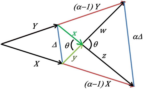
Let $d=d_T\left(X,Y\right)$ be the Thompson metric between (positive definite) matrices $X$ and $Y$ and let $\alpha =e^d$. Note that in Figure 1, which represents each matrix as a vector, all the vectors shown are coplanar. The angle $\theta$ is the same as the angle between $\alpha X-Y=x+z$ and $\alpha Y-X=y+w$. Since, by definition of the Thompson metric, $\alpha X-Y$ and $\alpha Y-X$ are both positive semidefinite, $\theta \le \frac{\pi }{2}\left(rad\right)$ and $tr\left(xy\right)$ and $tr\left(wz\right)\ge 0$ whereas $tr\left(xw\right)$ and $tr\left(yz\right)\le 0$. Thus, we have

(1) $\parallel \mathrm{\Delta }{{\parallel }_2}^2\le \parallel x{{\parallel }_2}^2+\parallel y{{\parallel }_2}^2$(1)

(2) $\parallel \alpha \mathrm{\Delta }{{\parallel }_2}^2\le \parallel w{{\parallel }_2}^2+\parallel z{{\parallel }_2}^2$(2)

(3) $\left(\alpha -1\right){X_2}^2\ge \parallel y{{\parallel }_2}^2+\parallel z{{\parallel }_2}^2$(3)

(4) $(\alpha -1)Y_2^2\ge \parallel w{\parallel }_2^2+\parallel x{\parallel }_2^2.$(4)

Figure 1. Relation of the Thompson metric to the Frobenius norm. This figure represents matrices X and Y as vectors that span a plane and illustrates the geometric intuition behind inequalities (1)–(4).

Adding inequalities (1) and (2) as well as (3) and (4), we have

$\parallel \mathrm{\Delta }{{\parallel }_2}^2+\parallel \alpha \mathrm{\Delta }{{\parallel }_2}^2\le \parallel x{{\parallel }_2}^2+\parallel y{{\parallel }_2}^2+\parallel w{{\parallel }_2}^2+\parallel z{{\parallel }_2}^2\le$

(5) $(\alpha -1)X_2^2+(\alpha -1)Y_2^2.$(5)

Thus

(6) $\parallel \mathrm{\Delta }{\parallel }_2^2+\parallel \alpha \mathrm{\Delta }{\parallel }_2^2\le (\alpha -1)X_2^2+\parallel (\alpha -1)Y{\parallel }_2^2.$(6)

Solving for $\parallel \mathrm{\Delta }{\parallel }_2$, we have our result

(7) $\parallel \mathrm{\Delta }{\parallel }_2\le \frac{\alpha -1}{\sqrt{1+{\alpha }^2}}\sqrt{\parallel X{\parallel }_2^2+\parallel Y{\parallel }_2^2}.$(7)

5. A generalization of the Frobenius (p = 2) case

Consider the related and more general problem of bounding the Frobenius norm $\parallel \mathrm{\Delta }{\parallel }_2$, with $\mathrm{\Delta }=X-Y$, given matrix bounds $X\le g\cdot Y$ and $Y\le f\cdot X$, for scalars $f$ and $g$. This generalization, illustrated in Figure 2, yields the following equations:

(8) $\parallel \mathrm{\Delta }{{\parallel }_2}^2=\parallel X{{\parallel }_2}^2+\parallel Y{{\parallel }_2}^2-2\parallel X{\parallel }_2\parallel Y{\parallel }_2\cdot cos\varphi$(8)

$\parallel {\mathrm{\Delta }}_{fg}{ }_2^2=\parallel f\cdot X{{\parallel }_2}^2+\parallel g\cdot Y{{\parallel }_2}^2-2\parallel f\cdot X{\parallel }_2\parallel g\cdot Y{\parallel }_2\cdot cos\varphi =\dots$

(9) $f^2\cdot \parallel X{\parallel }_2^2+g^2\cdot \parallel Y{\parallel }_2^2-2fg\parallel X{\parallel }_2\parallel Y{\parallel }_2\cdot cos\varphi .$(9)

Figure 2. Difference and Frobenius norm between two vectors give matrix bounds. This figure represents matrices X and Y as vectors that span a plane and illustrates the geometric intuition behind Equations (8) and (9) as well as inequality (10).

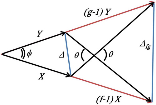
Similar to the argument above (in part 4), $X\le g\cdot Y$ and $Y\le f\cdot X$ imply that $\theta \le \frac{\pi }{2}\left(rad\right)$, which implies

$\parallel \mathrm{\Delta }{{\parallel }_2}^2+{\cdot }_{fg}{ }_2^2\le {\left(\parallel g\cdot Y{\parallel }_2-\parallel Y{\parallel }_2\right)}^2+{\left(\parallel f\cdot X{\parallel }_2-\parallel X{\parallel }_2\right)}^2=\dots$

(10) ${(f-1)}^2\cdot \parallel X{\parallel }_2^2+{(g-1)}^2\cdot \parallel Y{\parallel }_2^2.$(10)

The above system of two quadratic equations and one quadratic inequality has (assuming $\parallel X{\parallel }_2$ is known, even if $X$ is an unknown, approximated by $Y$) three unknowns: $\parallel \mathrm{\Delta }{\parallel }_2$, $\parallel {\mathrm{\Delta }}_{fg}{\parallel }_2$ and $cos\varphi$. Solving this system and simplifying the resulting solutions with Mathematica (Wolfram Research I, 2016) yields the following inequalities:

(11) $\parallel \mathrm{\Delta }{\parallel }_2\le \sqrt{\frac{\left(1+f\left(g-2\right)\right)\cdot \parallel X{{\parallel }_2}^2+\left(1+g\left(f-2\right)\right)\cdot \parallel Y{{\parallel }_2}^2}{1+f\cdot g}}$(11)

(12) $\parallel {\mathrm{\Delta }}_{fg}{{\parallel }_2}^2\le \sqrt{\frac{\left[f^2\cdot \left(\left(f-2\right)\cdot g+1\right)\right]\cdot \parallel X{{\parallel }_2}^2+\left[g^2\cdot \left(\left(g-2\right)\cdot f+1\right)\right]\cdot \parallel Y{{\parallel }_2}^2}{1+f\cdot g}}$(12)

(13) $cos\varphi \ge \frac{f\cdot \parallel X{\parallel }_2^2+g\cdot \parallel Y{\parallel }_2^2}{1+f\cdot g\cdot \parallel X{\parallel }_2\cdot \parallel Y{\parallel }_2}.$(13)

Note that this not only establishes a bound for $\parallel X-Y{\parallel }_2$, given matrix bounds $X\le g\cdot Y$ and $Y\le f\cdot \sqrt{b^2-4ac}\cdot X$, but this analysis also yields a bound for $cos\varphi$. Thus, this analysis provides information about the inner product between $X$ and $Y$, even in cases where $X$ is an unknown, approximated by $Y$. Of course, when $f=g=\alpha =e^d$, (11) simplifies to the result established in Section 4.

6. Numerical results

Fifty calculations, performed in MATLAB, with pairs of random positive definite $5\times 5$ matrices tested the tightness of the bounds presented in this paper. The following formulas generated the i^th pair $\left(X_i,Y_i\right)$ of matrices

(14) $X_i=\left(A+\left(i^2/100\right)\cdot B\right){\left(A+\left(i^2/100\right)\cdot B\right)}^T+D$(14)

(15) $Y_i=(A+(i^2/100)\cdot C){(A+(i^2/100)\cdot C)}^T+D,$(15)

where A, B and C have elements randomly drawn from the uniform distribution on [0,1] and D is a diagonal matrix with diagonal elements randomly drawn from that same distribution. The occurrence of the index i in the formula ensured a range of distances among the 50 matrix pairs tested.

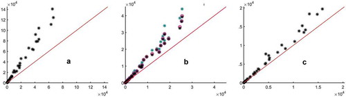
Figure 3 compares values of $X_i-{Y_i}_p$ for (A) p = 1 (trace norm), (B) p = 2 (Frobenius norm) and (C) p = ∞ (spectral norm) with bounds for those values calculated using Theorem 3.5, (and for panel B) Equation (7) and Equation (11). The function, thompson_metric.m, used to calculate the Thompson metric as well as f and g in Equation (11) is available via MATLAB Central File Exchange, and the script, and data calculated using that script, used to generate Figure 3 is available from the author upon request. While the bounds described in this paper are clearly not very tight (for matrices more distant from each other), hopefully, these results will spark further research leading to tighter bounds on Schatten norms based on the Thompson metric.

Figure 3. Comparison, for 50 pairs of matrices, of values of bounds for Schatten metrics derived in this paper vs. the values of the corresponding Schatten metric: (A) bound given by Theorem. 3.5 for the trace norm vs. the trace norm itself, (B) bounds for the Frobenius norm vs. the Frobenius norm itself and (C) bound given by Theorem. 3.5 for the spectral norm vs. the spectral norm itself. In panel (B), bounds given by Theorem. 3.5 are indicated with cyan markers, bounds given by Equation (7) are indicated with magenta markers, and bounds given by Equation (11) are indicated with black markers.

7. Discussion

Weyl’s inequalities, and hence some knowledge of the spectra of $X$ and $Y$, form the backbone of the proofs presented above. In the motivating case where $Y$ is an approximation of an unknown $X$, the spectrum of $X$ may also be unknown. While the principle result of this paper ultimately only requires knowledge of $\parallel X{\parallel }_p$ (as well as $\parallel Y{\parallel }_p$, which is generally known), purely geometric/trigonometric proofs, such as the one given for the Frobenius case, of the results presented in this paper would be more elegant given the nature of the motivating problem.

Furthermore, proofs not based on the matrix structure of $X$ and $Y$ but based purely on the ordering (Löwner ordering in this case) and norm (Schatten p-norm) being compared might allow for tighter bounds on $\parallel X-Y{\parallel }_p$ even in the absence of any knowledge of the spectrum of $X$ (or even of $Y$, for that matter), other than perhaps a restriction that $X$ and $Y$ be positive semidefinite. In comparison, Theorem 3.4 provides a tighter bound on $\parallel X-Y{\parallel }_p$ than the main result (Theorem 3.5), but it requires some knowledge of the spectrum of $X$ (at least that its eigenvalues are lower in magnitude than the corresponding eigenvalues of $Y$).

Additionally, proofs not based on the matrix structure of $X$ and $Y$ may lead to the generalization of these results in other orderings, which can also induce Thompson metrics (Cobzaş & Rus, 2014), and other norms. For instance, since the Frobenius norm arises from an inner product, a geometrically flavored argument leads to a slightly tighter bound on $\parallel X-Y{\parallel }_2$ than obtained from the general bound for $\parallel X-Y{\parallel }_p$ and setting $p=2$. On the other hand, the already established general result for a Thompson metric induced by a normal cone in a Banach space (Lemmens & Nussbaum, 2012; Nussbaum, 1988) is not as tight as the main result (Theorem 3.5) presented here: as $ϵ\to 0,$ the value of $\delta$ such that $0\le X\le \left(X+ϵI\right)\Rightarrow \parallel X\parallel \le \delta \parallel X+ϵI\parallel$ approaches unity; thus, the normality constant for the cone of positive semidefinite matrices is unity, and the general result for Banach spaces reduces to $\parallel X-Y\parallel \le 3\left(e^{d_T\left(X,Y\right)}-1\right)max\left[\parallel X\parallel ,\parallel Y\parallel \right]$, the right-hand side of which inequality is clearly greater than $2^{\frac{1}{p}}\frac{\left(e^d-1\right)}{e^d}max\left[\parallel X{\parallel }_p,\parallel Y{\parallel }_p\right]$ since $2^{\frac{1}{p}}\le 2<3$ and $e^d\ge 1$ since the (Thompson) metric $d$ is non-negative.

As illustrated in Section 5 of this paper, more general analysis of the Frobenius case yields not only a bound for $\parallel X-Y{\parallel }_2$ but also bounds inner product between $X$ and $Y$. In the case where $X$ is an unknown, approximated by $Y$, bounds on the inner product between $X$ and $Y$ further quantify how well $Y$ approximates $X$, and may provide further insight into improved approximations of an unknown $X$.

Hopefully, future research can further generalize the analysis presented in Section 5 to cases where $X\le g\left(Y\right)$ and $Y\le f\left(X\right)$, for more general classes of functions on $X$ and $Y$ than mere scalar multiplication. Such inequalities, in the Löwner order, arise, for example, in characterizing approximate solutions to the continuous algebraic Riccati equation (Zhang & Liu, 2010). Further generalization of the results presented here will facilitate expressing the quality of approximations, found in many areas of matrix algebra and optimization theory, in terms of geometrically intuitive metrics based on Schatten norms rather than less geometrically intuitive bounds in the Löwner order.

Acknowledgements

This work was made possible by the support of William Paterson University of NJ’s Office of the Provost for Assigned Release Time for research. The author also thanks Rajendra Bhatia as well as Yongdo Lim for their advice about where to submit this work and an anonymous reviewer for referring me to Lemmens’ and Nussbaum’s related results in nonlinear Perron-Frobenius theory.

Disclosure Statement

The author has no competing interests to declare.

Additional information

Funding

This work was not funded by any external granting agency or funding source. The author thanks the Department of Chemistry at William Paterson University for providing funding to maintain the author’s MATLAB license.

Notes on contributors

David A. Snyder

David A. Snyder is a professor in the Department of Chemistry at William Paterson University of NJ. He received a Bachelor of Science – double majoring in Mathematics and Biology – from the University of California, Irvine and a Ph.D. in Biochemistry from Rutgers University. Prior to starting his current position, Dr. Snyder was a post-doctoral researcher in Rafael Brüschweiler’s (then at Florida State University) research group. Dr. Snyder’s research interests include quantifying protein flexibility and covariance NMR, which comprises a family of techniques that use algebraic operations to enhance and combine NMR spectra. In the course of researching the accuracy of covariance NMR, Dr. Snyder found that many relevant algebraic results involved Thompson metrics rather than more intuitive metrics based on Schatten norms. The sparsity of mathematical literature relating Thompson metrics and Schatten norms prompted Dr. Snyder to prove the results presented in this paper.

References

- Baksalary, J. K., & Pukelsheim, F. (1991). On the Löwner, minus, and star partial orderings of nonnegative definite matrices and their squares. Linear Algebra and Its Applications, 151, 135–10. doi:10.1016/0024-3795(91)90359-5
- Bhatia, R. (2007). Perturbation bounds for matrix eigenvalues. Philadelphia, PA: SIAM.
- Carli, F. P., & Sepulchre, R. (2015). On the projective geometry of Kalman filter. Proceedings of the 54th Annual IEEE Conference on Decision and Control (CDC) (2420–2425). IEEE Online: IEEE-Xplore 2016 doi:10.1109/CDC.2015.7402570.
- Cobzaş, Ş. & Rus, M. (2014). Normal cones and Thompson metric. In T. Rassias & L. Tóth (Eds.), Topics in mathematical analysis and applications. Springer optimization and its applications (Vol. 94, pp. 209–258). New York, NY: Springer.
- Del Moral, P., Kurtzmann, A., & Tugaut, J. (2017). On the stability and the uniform propagation of chaos of a class of extended ensemble Kalman-Bucy filters. SIAM Journal on Control and Optimization, 55, 119–155. doi:10.1137/16M1087497
- Gaubert, S., & Qu, Z. (2014). The contraction rate in Thompson’s part metric of order-preserving flows on a cone – Application to generalized Riccati equations. Journal of Differential Equations, 256(8), 2902–2948. doi:10.1016/j.jde.2014.01.024
- Lawson, J., & Lim, Y. (2007). A Birkhoff contraction formula with applications to Riccati equations. SIAM Journal on Control and Optimization, 46(3), 930–951. doi:10.1137/050637637
- Lee, H., & Lim, Y. (2008). Invariant metrics, contractions and nonlinear matrix equations. Nonlinearity, 21(4), 857. doi:10.1088/0951-7715/21/4/011
- Lemmens, B., & Nussbaum, R. D. (2012). Nonlinear Perron-Frobenius theory. (Cambridge Tracts in Mathematics; 189). New York (NY): Cambridge University Press.
- Lemmens, B., & Roelands, M. (2015). Unique geodesics for Thompson’s metric [Les géodésiques uniques de la métrique de Thompson]. In: Annales De L’institut Fourier, 65, 315–348.
- Liao, A., Yao, G., & Duan, X. (2010). Thompson metric method for solving a class of nonlinear matrix equation. Applied Mathematics and Computation, 216(6), 1831–1836. doi:10.1016/j.amc.2009.12.022
- MathWorks I. MATLAB. MathWorks; 2017.
- Montrucchio, L. (1998). Thompson metric, contraction property and differentiability of policy functions. Journal of Economic Behavior & Organization, 33(3), 449–466. doi:10.1016/S0167-2681(97)00069-3
- Nussbaum, R. D. (1988). Hilbert’s projective metric and iterated nonlinear maps. (AMS Memoirs; Vol. 75, Number 391). Providence (RI): American Mathematical Society.
- Nussbaum, R. D., & Walsh, C. (2004). A metric inequality for the Thompson and Hilbert geometries. Journal of Inequalities in Pure and Applied Mathematics, 5. http://emis.ams.org/journals/JIPAM/images/131_03_JIPAM/131_03_www.pdf
- Qu, Z. (2014). Contraction of Riccati flows applied to the convergence analysis of a max-plus curse-of-dimensionality–Free method. SIAM Journal on Control and Optimization, 52(5), 2677–2706. doi:10.1137/130906702
- Weyl, H. (1949). Inequalities between the two kinds of eigenvalues of a linear transformation. Proceedings of the National Academy of Sciences of the United States of America, 35(7), 408–411. doi:10.1073/pnas.35.7.408
- Wolfram Research I. (2016). Mathematica. [Internet]. Champaign, Illinois: Wolfram Research, Inc.
- Yang, X. (2000). A matrix trace inequality. Journal of Mathematical Analysis and Applications, 250(1), 372–374. doi:10.1006/jmaa.2000.7068
- Yang, X. M., Yang, X. Q., & Teo, K. L. (2001). A matrix trace inequality. Journal of Mathematical Analysis and Applications, 263(1), 327–331. doi:10.1006/jmaa.2001.7613
- Zhang, J., & Liu, J. (2010). Matrix bounds for the solution of the continuous algebraic Riccati equation. Mathematical Problems in Engineering, 2010, 1–15. doi:10.1155/2010/819064