Prevention strategy for superinfection mathematical model tuberculosis and HIV associated with AIDS

Abstract

In this article, we extended the co-infection mathematical model [1] for optimal control purpose. We initially derived a threshold number $R_0$ and found bounded and biological region for the study of the proposed model. Here, we developed a methodology through the considered superinfection problem which is getting abate while neglecting Acquired Immuno deficiency Syndrome (AIDS) because it is a noncurable disease. For this, we developed the following control variables in our model: $V_1$, using treatment against TB; $V_2$, infection control in health-care center; $V_3$, co-treatment of multidrug-resistant TB and HIV or start both HIV antiretroviral and anti-TB drug therapy; and $V_4$, avoid close contact with TB patient. These are defined with some different schemes to minimize and control the infection from any community and population. In the last section, numerical simulation is presented which supports the given model.

Keywords:

• mathematical model
• threshold number
• sensitivity analysis
• biological region
• optimal control
• TB/HIV/AIDS
• numerical simulation

PUBLIC INTEREST STATEMENT

In this study we discussed the three acting play diseases AIDS/HIV/TB. Tuberculosis (TB) is a potentially serious infectious disease which bring HIV and then AIDS if no treatment taken. Here all the diseases are so harmful and transmissible, even if an individual get infection it transmit and circulate in the entire world. In this study we shown that vaccination is key factor against these diseases. The study is valuable for all mankind to avoid from these virus need to adopt good and healthy environment, isolation from infected individuals, vaccination at proper time etc. The study also provide a wide range of safety if precaution are adopted in advance, and if infected should be treated on time, is the necessary advise for all mankind.

1. Introduction and related literature

Mathematical models have a great role in science field. Developing a mathematical model is termed mathematical modeling which is used in natural sciences such as physics, chemistry, and biology, as well as in engineering sciences such as computer sciences and electrical sciences. It is the art to transfer any problems from application area into tractable mathematical formulation. Developing a mathematical models is the process that uses maths to represent, analyze, make predictions, or otherwise provide insight into the real-world phenomena. There are many mathematical models and many techniques to solve a particular problem. Mathematical biology can help us solve massive problems such as recycling option or the spread of a disease in a population. Work in mathematical biology is typically a collaboration between mathematician and biologist. Similarly, control of an infectious disease is obligatory; therefore, some mathematical models and methodology are adopted to control infection. This is known as optimal control.

1.1. AIDS/HIV/TB

AIDS is also called acquired immune deficiency syndrome which is occurred by a condition called spectrum. In the initial stage, AIDS patients show no clear symptoms or influenza-like illness (International Committee on Taxonomy of Viruses, 2002b). The most important fact about AIDS is that it takes a long time period for symptoms to be obvious (HIV/AIDS Fact sheet N360, 2015). While the late symptoms brought a viral infection called Acquired Immunodeficiency Syndrome (AIDS) (HIV/AIDS Fact sheet N360, 2015). AIDS can be spread by unprotected sex, blood transfusion, and usable syringes and from mother to child during pregnancy and breastfeeding which are the two major ways (About HIV/AIDS, 2015). Nowadays AIDS has no proper cure; however, antiretroviral vaccines have been developed which have a low infection rate, thus enabling AIDS patients to possess a near-normal life (Cunningham, Donaghy, Harman, Kim, & Turville, 2010). The total survival time without treatment for AIDS individual is 11 years after infection (Markowitz, edited by William N. Rom; associate editor, Steven B, 2007). Approximately 36.7 million individuals are living with HIV infection, while 1 million deaths occurr according to a survey conducted in 2016 (UNAIDS, WHO, 2007), and these infected people mostly live in sub-Saharan Africa (UNAIDS, WHO, 2007). Then, according to a 2014 survey, AIDS caused an estimated 39 million deaths worldwide (Fact sheet—Latest statistics on the status of the AIDS epidemic | UNAIDS, 2017). Initial infection with HIV is called acute HIV syndrome (Basic Statistics, 2015), while the next stage is called clinical latency. Without treatment in the second stage of HIV, the survival time is considered to be 3–20 years (Evian, 2006; xxxxx, 2007). The third chronic and last stage is called AIDS which can be defined as when the CD4 + T cells go down below 200 cells per µL (Duoyi, 2001). A recent study about AIDS was presented by Win Min Han et al. on 27 September 2018 which was related to CD4 and CD8 cell normalization and Tahir et al. presented a coinfection model (Tahir, Shah, & Zaman, 2018; Win Min et al., 2018). Optimal control theory is one of the powerful tools used in mathematics to control or reduce infection in the community and population. In this situation, a control law is required through which we judge the problem and minimize the infection.

Human immunodeficiency virus is a global health problem which is a lentivirus and causes HIV infection. It is one of the most studied infectious diseases in the world. If an infected individual does not use medicines against HIV, then the total survival time of that individualis 9–11 years (Lawn & Zumla, 2011). HIV is differentiated into two forms: HIV-1 and HIV-2. HIV-1 virus which was initially discovered is considered that mostly infect HIV globally (Doitsh et al., 2014). Transmission rate of HIV-2 mainly occurred in West Africa (International Committee on Taxonomy of Viruses, 2002a). A recent work on optimal control in 2018 has been done by Tahir el.al who presented the stability and optimal control of Middle East respiratory syndrome corona virus (MERS-CoV) (Tahir et al., 2018). HIV destroyed the system of basic immune cells of the human body system, like helper T cells (UNAIDS, WHO, 2007), and it decreases the numbers of CD4 + T cells by a mechanism called pyroptosis and broadly infects T-cell apoptosis of uninfected cells of the body (UNAIDS, WHO, 2007). When CD4 + T cells of a person decrease below the critical numbers, the body is prone infections (Cunningham et al., 2010). An optimal control was presented by Adams et al. HIV dynamics modeling, data analysis, and optimal treatment protocols (Duoyi, 2001) were discussed. Also for the optimal control purposes Hem Raj Joshi et al. discussed the optimal control of an HIV immunology model (Evian, 2006). Recently, Ciaranello et al. presented simulation modeling and metamodeling to explain national and international HIV policies for children and adolescents (WHO, 2007).

Tuberculosis (TB) is an infectious disease usually caused by the bacterium Mycobacterium tuberculosis (Tahir & Shah, 0000) and simply known as a contagious infection. TBgenerally affects the lungs. Most TB patients show no symptoms, and this is known as latent TB. Latent TB individuals are not harmful to people and do not spread the infection further. A tool to diagnose latent TB such as the tuberculin skin test (TST) is used. Nowadays, most TB cases are considered curable by the use of antibiotics. The latent infections progress into active TB in about 10% of the cases. Symptoms for the active TB include feeling of sickness, weight loss, high fever, cough, chest pain, and chronic cough containing blood or sputum. Medicines are prescribed for a period of 6 to 9 months. TB also spreads in the community by breathing contaminated air. According to a survey, one-third of the population of the entire world were considered to be infected by TB (Tahir & Shah, 0000), and some infections occur in about 1% of the whole population of the world every year (Tuberculosis Fact sheet N104, 2015). There has been a decline in the new cases of active TB from 2000 (Tahir & Shah, 0000). Also, 80% of the people in Asian and African countries show a positive test, while 5–10% people in the United States show a positive tuberculin test (Tuberculosis, 2002). TB disease was present in humans from ancient times (Kumar, Abbas, Fausto, & Mitchell, 2007). The optimal control strategy of a fractional multistrain TB model was presented by Sweilam, and Mekhlafi (Sweilam & Mekhlafi, 2016). Similarly, a numerical approach for optimal control was presented by (Sweilam & Mekhlafi, 2016) for the time delay of multistrain fractional model TB.

In this article, we extended the mathematical model (Tahir & Shah, 0000) and focus on the minimization of the superinfection AIDS, HIV,and TB problem. After the introduction and related literature, we find the threshold number. Then, we find the bounded and physical region for the study of the model. Here our mission is to control the infection,and for this purpose we defined four control variables ($V_1,V_2,V_3$,and $V_4$) which are characterized as follows: using treatment against TB, infection control in health-care center, co-treatment of multidrug-resistant TB and HIV or start both HIV antiretroviral, and anti-TB drug therapy and avoid close contact with TB patient. These are defined with some different schemes to minimize and control the infection from any population. We show numerical simulation for system (1) in the last section of the article with and without vaccination or control. From the simulation, we observed that the recovery is very fast in case of vaccination as compared to nonvaccination.

2. Related materials and problem’s formulation

This section contains a mathematical model for superinfection, that is, AIDS/HIV/TB, with three mutual infectious classes. Here, the population model is based on superinfection characteristics of AIDS, HIV infection, TB-HIV chronic stage, and the final AIDS (HIV) infection transmission stage. For this order, the whole population model is divided into nine mutual relations as:

1. Susceptible individuals are represented by $R_1(t)$ who are not infected, but with a chance to get infection.

2. Latent TB individuals are represented by $R_2(t)$ with no symptoms of TB.

3. Active TB individuals are represented by $R_3(t)$ with TB infection.

4. Recovered TB individuals assigned by $R_4(t)$.

5. HIV-infected individuals represented by $R_5(t)$ with no symptoms of AIDS.

6. HIV-infected individuals having AIDS symptom are represented by $R_6(t)$.

7. HIV-infected individuals represented by $R_7(t)$ which are under the treatment of HIV infection.

8. TB latent individuals represented by $R_8(t)$ with co-infected HIV (pre-AIDS).

9. HIV-infected individuals (pre-AIDS) represented by $R_9(t)$ and having active TB symptoms also.

Now all the assumptions from $1$ to $9$ lead a compartmental mathematical model with the following differential equations:

$R_1^{\bullet }(t)=\mu -\mathrm{\Pi }(t)R_1(t)-\mathrm{\Xi }(t)R_1(t)-d_N{R}_1(t),$

$R_2^{\bullet }(t)=\mathrm{\Pi }(t)S(t)+{\gamma }_1\mathrm{\Pi }(t)R_3(t)-(k_1+{\tau }_1+d_N)R_2(t),$

$R_3^{\bullet }(t)=k_1{R}_2(t)-({\tau }_2+d_T+d_N+\delta \mathrm{\Xi }(t))R_3(t),$

(1) $R_4^{\bullet }(t)={\tau }_1{R}_2(t)+{\tau }_2{R}_3(t)-({\gamma }_1\mathrm{\Pi }(t)+\mathrm{\Xi }(t)+d_N)R_4(t),$(1)

$R_5^{\bullet }(t)=\mathrm{\Xi }(t)R_1(t)-({\rho }_1+\varphi +\psi \mathrm{\Pi }(t)+d_N)R_5(t))+{\alpha }_1{R}_6(t)+\mathrm{\Xi }(t)R_4(t)+{\omega }_1{R}_7(t),$

$R_6^{\bullet }(t)={\rho }_1{R}_5(t)+{\omega }_2{R}_{10}(t)-{\alpha }_1{R}_6(t)-(d_N+d_A)R_6(t),$

$R_7^{\bullet }(t)=\varphi R_5(t)+u_1(t){\rho }_2{R}_9(t)+r{k}_3{R}_8(t)-({\omega }_1+d_N)R_7(t),$

$R_8^{\bullet }(t)={\gamma }_2\mathrm{\Pi }(t)R_{10}(t)-(k_2+k_3+d_N)R_8(t),$

$R_9^{\bullet }(t)=\delta \mathrm{\Xi }(t)R_3(t)+\psi \mathrm{\Pi }(t)R_5(t)+{\alpha }_2{R}_6(t)+k_2{R}_8(t)-({\rho }_2+d_N+d_T)R_9(t).$

For the above system (1), we fix the following initial conditions as

$R_1(t)\ge 0,R_2(t)\ge 0,R_3(t)\ge 0,R_4\ge 0,R_5(t)\ge 0,R_6(t)\ge 0,R_7(t)\ge 0,$

$R_8(t)\ge 0,R_9(t)\ge 0.$

Also, we have drawn some certain assumptions in system $(1)$. They are as follows:

${\gamma }_1$, ${\gamma }_2$, ${\eta }_C$, ${\eta }_A$, $\delta$, and $\psi$ represent the modification parameters.

$\mu$ represents the recruitment rates,

${\beta }_1$ represents the TB transmission rate,

${\beta }_2$ represents the HIV transmission rate.

$k_1$ represents the rate of individuals who leave compartment $2$ by becoming infected.

$k_2$ represents the individuals who leave compartment $8$ and enter into the TB infection compartment.

$k_3$ represents the individual to move from compartment $8$.

${\rho }_1$ represents the rate in which the individuals leave compartment $5$ and enter into compartment $6$.

${\rho }_2$ individuals leave compartment $9$.

${\omega }_1$ represents the individual who leave compartment $7$.

${\omega }_2$ represents the individuals who leave compartment $9$.

${\tau }_1$ represents the TB individual treatment rate for compartment $2$ individuals.

${\tau }_2$ represents the treatment rate for compartment $3$ individuals.

$\varphi$ represents the HIV treatment rate for compartment $5$ individuals.

${\alpha }_1$ represent the AIDS treatment rate.

${\alpha }_2$ represents the HIV treatment rate for $9$ class individuals.

$r$ represents the fraction of $8$ individuals who used HIV and TB treatment.

$d_{T}A$ represents AIDS- and TB-induced death rate.

$d_T$ represents TB individual-induced death rate.

$d_N$ represents the natural death rate.

$d_A$ represents the AIDS individual-induced death rate.

The total population of system (1) at any time $t$ is represented by $P(t)$ as below,

$P(t)=R_1(t)+R_2(t)+r_3(t)+R_4(t)+R_5(t)+R_6(t)+R_7(t)+R_8(t)+R_9(t).$

We also assume that:

“Active TB” individuals infect susceptible individuals of “latent TB” by the rate of transmission $\mathrm{\Pi }$.

All individuals having HIV will infect susceptible individuals of HIV by a transmission rate $\mathrm{\Xi }$ as under,

$\mathrm{\Pi }(t)=\frac{{\beta }_1}{P(t)}(R_3(t)+R_9(t)+R_8(t)).$

The value of $\mathrm{\Xi }$ is as,

$\mathrm{\Xi }(t)=\frac{{\beta }_2}{P(t)}[R_4\mathrm{\Psi }4(t)+R_9(t)+R_8(t)+R_9(t)+{\eta }_C{R}_7(t)+{\eta }_A(R_6(t)+R_8(t))].$

Also we have drawn some more assumptions as:

${\beta }_1$ represents the effectiveness rate of TB-infected individuals

and ${\beta }_2$ represents the effectiveness rate of HIV-infected individuals.

η_A ≥ 1 represents the modification parameter relative infectiousness for AIDS symptom individuals.

η_c ≤ 1 represents the modification parameter of the body immunity for the individual suffered in HIV produced by anti-retroviral treatment.

3. Bounded and biological region

As the total population of model (1) is represented by $P(t)$, so differentiating the same and using values we get the following,

$\frac{dP(t)}{dt}\le \mu -d_{N}P(t).$

Thus, for biological study purposes, we study model (1) in the below closed region,

$\mathrm{\Psi }=\{(R_1(t),R_2(t),R_3(t),R_4(t),R_5(t),R_6(t),R_7(t),R_8(t),R_9(t)$

(2) $\in R_{+}^9,0<V\le \mu -d_{N}P(t)\}.$(2)

The value of “V” is as under,

$V=(R_1(t)+R_2(t)+R_3(t)+R_4(t)+R_5(t)+R_6(t)+R_7(t)+R_8(t)+R_9(t)).$

which shows that the proposed model is bounded and closed.

4. Calculation of reproductive number “$R_0$”

The reproductive number is considered as one of the important and fundamental key value in many epidemiological models, which is represented by $R_0$ which predicts whether the infectious disease will be spread into a population class or not. We define the basic reproduction number as “It shows average rate of a secondary infectious cases when ever one of infectious individual is introduced in susceptible population.” There are many approaches that are used to derive $R_0$ in an epidemiological mathematical model, but we used next-generation matrix concept which is interesting and also a very simple tool. The next-generation matrix is very useful tool to determine a biologically meaningful formula to find the basic reproduction number in the continuous epidemic model, (that is) system of differentials equations. By the next-generation matrix approach, the whole model is divided into two groups:

(1) infected and

(2) noninfected groups

Then, we define Jacobian matrix for infectious class and then Jacobian matrix is split further into two matrices, that is, $J=F-V$, where $J$ represents the Jacobian matrix and $F$, $V$ are the newly generated matrices. After this, we find the inverse of $V$ and multiply with matrix $F$, that is $F{V}^{-1}$. Finally, the most dominant eigen value is taken, which is the required basic reproduction number $R_0$. According to the statement above, the basic reproduction number for our system (1) is

$R_0=Max\left[\frac{\delta \mathrm{\Xi }(t)}{{\tau }_2+d_T+d_N},\frac{\psi \mathrm{\Pi }(t)}{{\rho }_1+\varphi +d_N}\right].$

The above $R_0$ is the required value of our model.

5. Optimal control problem of the proposed model

In mathematical models,the optimal control for any problem is considered one of the powerful tools through the complex structure of the dynamical system (Mandell & Dolan,2010). The said technique is used for the dynamics study of the disease, and for more details refer (Lenhart & Workman, 2007; Zaman, Kang, & Jung, 2009).It is also good to check (Khan et al., 2012, 2013a). Now to determine the optimal control to minimize the infected individuals and maximize the number of susceptible individuals and recovered individuals, we define six variables for 10 state variables, which are $R_1(t)$, $R_2(t)$, $R_3(t)$, $R_4(t)$, $R_5(t)$, $R_6(t)$, $R_7(t)$, $R_8(t)$, and $R_9(t)$. Here in equation (3) we define the control variables which are defined as follows:

$R_1^{\bullet }(t)=\mu -\mathrm{\Pi }(t)R_1(t)-\mathrm{\Xi }(t)R_1(t)-d_N{R}_1(t)$

$+V_1{L}_{TH}(t)+V_2{I}_T(t)+V_{3}R(t)+V_4{R}_H(t)+V_5{I}_{TH}(t)+V_{6}A(t),$

$R_2^{\bullet }(t)=\mathrm{\Pi }(t)S(t)+{\gamma }_1\mathrm{\Pi }(t)R_3(t)-(k_1+{\tau }_1+d_N)R_2(t)+V_1{L}_{TH}(t)+V_2{I}_T(t)+V_{3}R(t),$

$R_3^{\bullet }(t)=k_1{R}_2(t)-({\tau }_2+d_T+d_N+\delta \mathrm{\Xi }(t))R_3(t)+V_1{L}_{TH}(t)+V_2{I}_T(t)+V_{3}R(t),$

$R_4^{\bullet }(t)={\tau }_1{R}_2(t)+{\tau }_2{R}_3(t)-({\gamma }_1\mathrm{\Pi }(t)+\mathrm{\Xi }(t)+d_N)R_4(t)+V_2{I}_T(t),$

$R_5^{\bullet }(t)=\mathrm{\Xi }(t)R_1(t)-({\rho }_1+\varphi +\psi \mathrm{\Pi }(t)+d_N)R_5(t))+{\alpha }_1{R}_6(t)+\mathrm{\Xi }(t)R_4(t)+{\omega }_1{R}_7(t)$

$+V_1{L}_{TH}(t)+V_{3}R(t)+V_4{R}_H(t)+V_5{I}_{TH}(t),$

$R_6^{\bullet }(t)={\rho }_1{R}_5(t)+{\omega }_2{R}_{10}(t)-{\alpha }_1{R}_6(t)-(d_N+d_A)R_6(t)+V_1{L}_{TH}(t)+V_2{I}_T(t)+V_{3}R(t)$

(3) $+V_4{R}_H(t)+V_{6}A(t),$(3)

$R_7^{\bullet }(t)=\varphi R_5(t)+u_1(t){\rho }_2{R}_9(t)+r{k}_3{R}_8(t)-({\omega }_1+d_N)R_7(t)+V_1{L}_{TH}(t)+V_2{I}_T(t)$

$+V_{3}R(t)+V_4{R}_H(t)+V_5{I}_{TH}(t),$

$R_8^{\bullet }(t)={\gamma }_2\mathrm{\Pi }(t)R_{10}(t)-(k_2+k_3+d_N)R_8(t)+V_2{I}_T(t)+V_{3}R(t)+V_4{R}_H(t)+V_5{I}_{TH}(t),$

$R_9^{\bullet }(t)=\delta \mathrm{\Xi }(t)R_3(t)+\psi \mathrm{\Pi }(t)R_5(t)+{\alpha }_2{R}_6(t)+k_2{R}_8(t)-({\rho }_2+d_N+d_T)R_9(t)+V_1{L}_{TH}(t)$

$+V_2{I}_T(t)+V_{3}R(t)+V_4{R}_H(t)+V_5{I}_{TH}(t).$

Subjected to initial conditions of equation (2),the control variables $V_1,V_2,V_3$,and $V_4$ are assigned forusing treatment against TB, infection control in health-care center, co-treatment of multidrug-resistant TB and HIV or start both HIV antiretroviral and anti-TB drug therapy and avoid close contact with TB patient.

Now we define the objective function with the control problem which should minimize infection in all individuals as well as maximize susceptible and recovered individuals. To achieve the desired goal, we define five control variables mentioned above. So the required objective function with the control problem is:

$J(V_1,V_2,V_3,V_4)=min{\int }_0^{tend}[(Z_1{R}_1(t)+Z_2{R}_{@}(t)+Z_3{R}_3(t)+Z_4{R}_4(t)+Z_5{R}_5(t)+Z_6{R}_6(t)$

$+7R_7(t)+Z_8{R}_8(t)+Z_9{R}_9(t)$

$+$

(4) $+\frac{1}{2}\{W_1{V}_1^2(t)+W_2{V}_2^2(t)+W_3{V}_3^2(t)$(4)

$+W_4{V}_4^2(t))\}]dt$

In the above equation, we represent the terms $Z_1$, $Z_2$, $Z_3$, $Z_4$, $Z_5$, $Z_6$, $Z_7$, $Z_8$, and $Z_9$ as susceptible individuals; unexposed TB individuals; TB-infected individuals; TB recovered individuals with HIV but no symptom of AIDS individuals; both HIV and AIDS individuals; treatment of HIV-,TB-, and HIV-infected individuals; TB and HIV having no AIDS individuals; TB and HIV recovered with no AIDS individuals and HIV having AIDS individuals, respectively. Our mission is to maximize the number of recovered individuals in the population and also we try to minimize all the infected individuals. To achieve the goal, we will define the following control set. Also in equation $(4)$,the terms used are classified as follows:

$\bullet$ $\frac{1}{2}(W_1{V}_1^2)$ using treatment against “TB,”

$\bullet$ $\frac{1}{2}(W_2{V}_2^2)$ using to avoid close contact with “TB” patient,

$\bullet$ $\frac{1}{2}(W_3{V}_3^2)$ using for co-treatment of multidrug-resistant “TB” and “HIV”

or

start both “HIV” antiretroviral and anti “TB” drug therapy,

$\bullet$ $\frac{1}{2}(W_4{V}_4^{2}0)$ using for infection control in the health-care center.

Now to find control function for the above, we processed as below:

$J(V_1^{\ast },V_2^{\ast },V_3^{\ast },V_4^{\ast })=min\{J(V_1,V_2,V_3,V_4)\}$ such that $(V_1,V_2,V_3,V_4$)$\epsilon Q$

Control set for the system (3) is defined as,

$Q$=$\{(V_1,V_2,V_3,V_4/V_i(t)$ is lebesgue measure on $[1,0],0\le V_i(t)<1$

where (i = 1,2,3,4)

6. Existence of the optimal control problem of the model

By considering the control system (4) at any time $t=0$ now to show the existence of the optimal control problem, we define Equation (5) and (6) by “Lagrangian” and “Hamiltonian”. First, we need to define the Lagrangian for the optimal control problem, as under,

$L(R_1,R_2,R_3,R_4,R_5,R_6,R_7,R_8,R_9)=Z_1{R}_1(t)+Z_2{R}_2(t)+Z_3{R}_3(t)+Z_4{R}_4(t)+Z_5{R}_5(t)$

$+Z_6{R}_6(t)+Z_7{R}_7(t)+Z_8{R}_8(t)+Z_9{R}_9(t)$

$+\frac{1}{2}(W_1{V}_1^2+W_2{V}_2^2+W_3{V}_3^2+W_4{V}_4^2).$

Now for the optimal control, we define the “Hamiltonian “H” as given below,

$H=L(R_1,R_2,R_3,R_4,R_5,R_6,R_7,R_8,R_9)+{\xi }_1\left(\frac{d}{dt}{R}_1(t)\right)+{\xi }_2\left(\frac{d}{dt}{R}_2(t)\right)+{\xi }_3\left(\frac{d}{dt}{R}_3(t)\right)$

$+{\xi }_4\left(\frac{d}{dt}{R}_4(t)\right)+{\xi }_5\left(\frac{d}{dt}{R}_5(t)\right)+{\xi }_6\left(\frac{d}{dt}{R}_6(t)\right)+{\xi }_7\left(\frac{d}{dt}{R}_7(t)\right)+{\xi }_8\left(\frac{d}{dt}{R}_8(t)\right)+{\xi }_9\left(\frac{d}{dt}{R}_9(t)\right).$

Now optimal control existence is given by,

$H=L+{\xi }_1[\mu -\mathrm{\Pi }(t)R_1(t)-\mathrm{\Xi }(t)R_1(t)-d_N{R}_1(t)]+{\xi }_2[\mathrm{\Pi }(t)S(t)+{\gamma }_1\mathrm{\Pi }(t)R_3(t)-(k_1+{\tau }_1+d_N)R_2(t)]$

$+{\xi }_3[k_1{R}_2(t)-({\tau }_2+d_T+d_N+\delta \mathrm{\Xi }(t))R_3(t)]+{\xi }_4[{\tau }_1{R}_2(t)+{\tau }_2{R}_3(t)-({\gamma }_1\mathrm{\Pi }(t)+\mathrm{\Xi }(t)+d_N)R_4(t)]$

$+{\xi }_5[\mathrm{\Xi }(t)R_1(t)-({\rho }_1+\varphi +\psi \mathrm{\Pi }(t)+d_N)R_5(t))+{\alpha }_1{R}_6(t)+\mathrm{\Xi }(t)R_4(t)+{\omega }_1{R}_7(t)]+$

$+{\xi }_6[{\rho }_1{R}_5(t)+{\omega }_2{R}_8(t)-{\alpha }_1{R}_6(t)-(d_N+d_A)R_6(t)]+{\xi }_7[\varphi R_5(t)+u_1(t){\rho }_2{R}_9(t)+r{k}_3{R}_8(t)$

(5) $-({\omega }_1+d_N)R_7(t)]+{\xi }_8[{\gamma }_2\mathrm{\Pi }(t)R_8(t)-(k_2+k_3+d_N)R_8(t)]$(5)

$+{\xi }_9[\delta \mathrm{\Xi }(t)R_3(t)+\psi \mathrm{\Pi }(t)R_5(t)+{\alpha }_2{R}_6(t)+k_2{R}_8(t)-({\rho }_2+d_N+d_T)R_9(t)]$

$+{\xi }_8[u_2(t){\rho }_2{R}_9(t)+(1-r)k_3{R}_8(t)-({\gamma }_2\mathrm{\Pi }(t)+{\omega }_2+d_N)R_8(t)]$

$+{\xi }_9[(1-(u_1(t)+u_2(t))){\rho }_2{R}_9(t)-({\alpha }_2+d_N+d_{TA})R_9(t)].$

where the value of “Lagrangian”,that is “L,” is given as,

$L=Z_1{R}_1(t)+Z_2{R}_2(t)+Z_3{R}_3(t)+Z_4{R}_4(t)+Z_5{R}_5(t)$

$+Z_6{R}_6(t)+Z_7{R}_7)t+Z_8{R}_8(t)+Z_9{R}_9(t)$

(6) $+\frac{1}{2}(W_1{V}_1^2+W_2{V}_2^2+W_3{V}_3^2+W_4{V}_4^2).$(6)

Now for the existence of the proposed model, we have the following known result, Theorem 8.1. For existence of optimal control we take, $u^{\star }=(V_1^{\star },V_2^{\star },V_3^{\star },V_4^{\star })$ $\epsilon Q$, such that,

$L(V_1^{\star },V_2^{\star },V_3^{\star },V_4^{\star })$ $=minL(V_1^{\star },V_2^{\star },V_3^{\star },V_4^{\star })$,

subjected to initial conditions of the control system (2).

Proof: Now to prove the optimal control existence using in (Fact sheet—Latest statistics on the status of the AIDS epidemic | UNAIDS, 2017), we define positive control variables as well as state variables. To minimize the case defined above, the convexity required for the objective functional in Equations (4), $V_1(t),V_2(t),V_3(t)$, and $V_4(t)$ is are satisfied. The set of control variables $V_1(t),V_2(t),V_3(t)$, and $V_4(t)$ $\epsilon$ $W$ so by the definition it is closed and also convex. Here optimal control system is bounded which shows the compactness and fulfills the existence of the proposed model and optimal control for further to integrand on objective functional (4),

$\begin{array}{rl}& L=Z_1{R}_1(t)+Z_2{R}_2(t)+Z_3{R}_3(t)+Z_4{R}_4(t)+Z_5{R}_5(t)+Z_6{R}_6(t)+Z_7{R}_7)t+Z_8{R}_8(t)\\ & \frac{1}{2}(W_1{V}_1^2+W_2{V}_2^2+W_3{V}_3^2+W_4{V}_4^2).\end{array}$

Taking the convex in optimal control, that is, set W which implies the ensure of optimal control, $(V_1^{\star },V_2^{\star },V_3^{\star },V_4^{\star })$ to minimize (3). For optimal control problem, we need to find optimal control solution for our purposed model. For this, we use maximum principle of Pontryagin's (Tuberculosis, 2002) to the Hamiltonian as below.

(7) $H(y,p(y),u(y),\lambda (y))=f(y,p(y),u(y)+\lambda (g(p(y),u(y))).$(7)

If $(p^{\star }$, $w_1^{\star }$, $w_2^{\star })$, $w_3^{\star })$, $w_4^{\star }))$, we will consider the optimal control solution for the required proposed optimal control problem then obviously a nontrivial vector exists,

$\lambda (y)=({\lambda }_1(y),{\lambda }_2(y),{\lambda }_3(y)....................,{\lambda }_n(y)).$

such that $y$ is taken for time, that is, $y=t$

$\frac{dx}{dy}=\mathrm{\partial }H(y,x(y),u(y),\lambda (y))$

(8) $0=\frac{\mathrm{\partial }H(y,p(t),u(y),u(y),\lambda (y)}{\mathrm{\partial }u}$(8)

$\lambda (y{)}^{\prime }=\frac{\mathrm{\partial }H(y,p(y),u(y),\lambda (y)}{\mathrm{\partial }x}.$

On Hamiltonian equation, we apply the necessary condition and we processed as below.

Theorem 8.2. Suppose that $R_1^{\star }(t),R_2^{\star }(t),R_3^{\star }(t),R_4^{\star }(t),R_5^{\star }(t),R_6^{\star }(t),R_7^{\star }(t),R_8^{\star }(t),R_9^{\star }(t)$ are the optimal state solution regarding to optimal control variables $V_1^{\star },V_2^{\star },V_3^{\star },V_4^{\star }$ for the optimal problem (4) also (3). Then the adjoint variables will exist there ${\lambda }_1(y),{\lambda }_2(y),{\lambda }_3(y),{\lambda }_4(y),{\lambda }_5(y),{\lambda }_6(y),{\lambda }_7(y),{\lambda }_8(y),{\lambda }_9(y)$ are satisfied.

${\lambda }_1^{\prime }(y)={\xi }_1({\lambda }_T(t)+{\lambda }_H(t)+dN)-({\xi }_2{\lambda }_T(t)+{\xi }_5{\lambda }_H(t)+Z_1),$

${\lambda }_2^{\prime }(y)={\xi }_2(k_1+{\tau }_1+dN)-({\xi }_3{k}_1+{\xi }_4{\tau }_1+Z_2),$

${\lambda }_3^{\prime }(y)={\xi }_3({\tau }_3+d_T+d_N+\delta {\lambda }_H(ty)-9{\xi }_4{\tau }_2+Z_3),$

${\lambda }_4^{\prime }(y)={\xi }_4({\gamma }_1{\lambda }_T(t)+{\lambda }_H(t)+d_N)-({\xi }_5{\lambda }_H(t)+Z_4),$

${\lambda }_5^{\prime }(y)={\xi }_5({\rho }_1+\varphi +\psi {\lambda }_T(t)+d_N)-({\xi }_6{\rho }_1+{\xi }_7\varphi +{\xi }_9\psi {\lambda }_T(t)),$

(9) ${\lambda }_6^{\prime }(y)={\xi }_6({\alpha }_1+d_N+d_A)-({\xi }_5{\alpha }_1+Z_6),$(9)

${\lambda }_7^{\prime }(y)={\xi }_7({\omega }_1+d_N)-({\xi }_5{\omega }_1+Z_7),$

${\lambda }_8^{\prime }(y)={\xi }_8(k_2+k_3+d_N)-({\xi }_{7}r{k}_3+{\xi }_9{k}_2+{\xi }_{10}(1-r)+Z_8),$

${\lambda }_9^{\prime }(y)={\xi }_9({\rho }_2+d_N+d_T)-({\xi }_7{\rho }_2{u}_1(t)+{\xi }_{10}{\rho }_2{u}_2(t)+{\xi }_{11}(1-u_1(t)+u_2(t)){\rho }_2).$

$with$ $the$ $transversality$ $conditions$ $(boundary$ $conditions).$

${\lambda }_i(y)=0$, for $i=1,2,3,4.$

$further$ $more$ $the$ $optimal$ $control$ $variables$ $V_1^{\ast }$, $V_2^{\ast }$, $V_3^{\ast }$ $and$ $V_4^{\ast }$ $are$ $as$:

(10) $\begin{array}{rl}& V_1^{\ast }=max\left\{min\left\{\frac{-7L_{TH}(t)}{W_1},1\right\},0\right\},\\ & V_2^{\ast }=max\left\{min\left\{\frac{-6I_T(t)}{W_2},1\right\},0\right\},\\ & V_3^{\ast }=max\left\{min\left\{\frac{-8R(t)}{W_3},1\right\},0\right\},\\ & V_4^{\ast }=max\left\{min\left\{\frac{-7R_H(t)}{W_4},1\right\},0\right\}.\end{array}$(10)

Proof: Now to find the adjoint Equation (3) for transversality conditions (8), let us consider $Hamiltonian$ (5) by representing $R_1(t)=R_1^{\star }(t),R_2(t)=R_2^{\star }(t),R_3(t)=R_3^{\star }(t),R_4(t)=R_4^{\star }(t),R_5(t)=R_5^{\star }(t),R_6(t)=R_6^{\star }(t),R_7(t)=R_7^{\star }(t),R_8(t)=R_8^{\star }(t),R_9(t)=R_9^{\star }(t)=0$ then differentiatial $Hamiltonian$ equation with respect to time$,S(t)$, $L_T(t)$, $I_T(t)$, $R(t)$, $I_H(t)$, $A(t)$, $C_H(t)$, $L_{TH}(t)$, and $I_{TH}(t)$. then we obtain the desired adjoint Equation (9). We find $V_1^{\ast }$, $V_2^{\ast }$, $V_3^{\ast }$, and $V_4^{\ast }$. Now differentiate the $Hamiltonian$ with respect to $V_1$, $V_2$, $V_3$ and $V_4$, we solve $\frac{\mathrm{\partial }H}{\mathrm{\partial }{V}_1}=0$, $\frac{\mathrm{\partial }H}{\mathrm{\partial }{V}_2}=0$, $\frac{\mathrm{\partial }H}{\mathrm{\partial }{V}_3}=0$, $\frac{\mathrm{\partial }H}{\mathrm{\partial }{V}_4}=0$, on the interior on the control set we use optimality conditions. Finally, we use property of the control space $W$ to get Equations (10) and (11) which completes the required proof.

Now from Equations (10) and (11) from the optimal control $V^{\ast }$ the characterization of the optimal control. We obtained the state variables and also optimal control variables by solving optimality system which contains state variables (4) and adjoint system (3) by boundary conditions (10) and (11).

Putting the values of $V_1^{\ast }$, $V_2^{\ast }$, $V_3^{\ast }$, and $V_4^{\ast }$, on the control system (3), we obtain the following.

$R_1^{\bullet }(t)=\mu -\mathrm{\Pi }(t)R_1(t)-\mathrm{\Xi }(t)R_1(t)-d_N{R}_1(t)$

$+max\left\{min\left\{\frac{-7L_{TH}(t)}{W_1},1\right\},0\right\}{L}_{TH}(t)+max\left\{min\left\{\frac{-6I_T(t)}{W_2},1\right\},0\right\}{I}_T(t)$

$+max\left\{min\left\{\frac{-8R(t)}{W_3},1\right\},0\right\}R(t)+max\left\{min\left\{\frac{-7R_H(t)}{W_4},1\right\},0\right\}{R}_H(t)$

$+max\left\{min\left\{\frac{-6I_{TH}(t)}{W_5},1\right\},0\right\}{I}_{TH}(t),$

$R_2^{\bullet }(t)=\mathrm{\Pi }(t)S(t)+{\gamma }_1\mathrm{\Pi }(t)R_3(t)-(k_1+{\tau }_1+d_N)R_2(t)$

$+max\left\{min\left\{\frac{-7L_{TH}(t)}{W_1},1\right\},0\right\}{L}_{TH}(t)+max\left\{min\left\{\frac{-6I_T(t)}{W_2},1\right\},0\right\}{I}_T(t)$

$+max\left\{min\left\{\frac{-8R(t)}{W_3},1\right\},0\right\}R(t),$

$R_3^{\bullet }(t)=k_1{R}_2(t)-({\tau }_2+d_T+d_N+\delta \mathrm{\Xi }(t))R_3(t)+ax\left\{min\left\{\frac{-7L_{TH}(t)}{W_1},1\right\},0\right\}{L}_{TH}(t)$

$+max\left\{min\left\{\frac{-6I_T(t)}{W_2},1\right\},0\right\}{I}_T(t)$

$+max\left\{min\left\{\frac{-8R(t)}{W_3},1\right\},0\right\}R(t),$

$R_4^{\bullet }(t)={\tau }_1{R}_2(t)+{\tau }_2{R}_3(t)-({\gamma }_1\mathrm{\Pi }(t)+\mathrm{\Xi }(t)+d_N)R_4(t)$

$+max\left\{min\left\{\frac{-6I_T(t)}{W_2},1\right\},0\right\}{I}_T(t),$

(11) $R_5^{\bullet }(t)=\mathrm{\Xi }(t)R_1(t)-({\rho }_1+\varphi +\psi \mathrm{\Pi }(t)+d_N)R_5(t))+{\alpha }_1{R}_6(t)+\mathrm{\Xi }(t)R_4(t)+{\omega }_1{R}_7(t)$(11)

$+max\left\{min\left\{\frac{-8R(t)}{W_3},1\right\},0\right\}R(t)+max\left\{min\left\{\frac{-7R_H(t)}{W_4},1\right\},0\right\}{R}_H(t)$

$+max\left\{min\left\{\frac{-6I_{TH}(t)}{W_5},1\right\},0\right\}{I}_{TH}(t),$

$R_6^{\bullet }(t)={\rho }_1{R}_5(t)+{\omega }_2{R}_8(t)-{\alpha }_1{R}_6(t)-(d_N+d_A)R_6(t)$

$+max\left\{min\left\{\frac{-7L_{TH}(t)}{W_1},1\right\},0\right\}{L}_{TH}(t)+max\left\{min\left\{\frac{-6I_T(t)}{W_2},1\right\},0\right\}{I}_T(t)$

$+max\left\{min\left\{\frac{-8R(t)}{W_3},1\right\},0\right\}R(t)+max\left\{min\left\{\frac{-7R_H(t)}{W_4},1\right\},0\right\}{R}_H(t)$

$+max\left\{min\left\{\frac{-6I_{TH}(t)}{W_5},1\right\},0\right\}{I}_{TH}(t)+max\left\{min\left\{\frac{-3A(t)}{W_6},1\right\}A(t),\right.$

$R_7^{\bullet }(t)=\varphi R_5(t)+u_1(t){\rho }_2{R}_9(t)+r{k}_3{R}_8(t)-({\omega }_1+d_N)R_7(t)+max\left\{min\left\{\frac{-6I_T(t)}{W_2},1\right\},0\right\}{I}_T(t)$

$+max\left\{min\left\{\frac{-8R(t)}{W_3},1\right\},0\right\}R(t)+max\left\{min\left\{\frac{-7R_H(t)}{W_4},1\right\},0\right\}{R}_H(t)$

$+max\left\{min\left\{\frac{-6I_{TH}(t)}{W_5},1\right\},0\right\}{I}_{TH}(t)+max\left\{min\left\{\frac{-3A(t)}{W_6},1\right\}A(t),\right.$

$R_8^{\bullet }(t)={\gamma }_2\mathrm{\Pi }(t)R_8(t)-(k_2+k_3+d_N)R_8(t)+max\left\{min\left\{\frac{-6I_T(t)}{W_2},1\right\},0\right\}{I}_T(t)$

$+max\left\{min\left\{\frac{-8R(t)}{W_3},1\right\},0\right\}R(t)+max\left\{min\left\{\frac{-7R_H(t)}{W_4},1\right\},0\right\}{R}_H(t)$

$+max\left\{min\left\{\frac{-6I_{TH}(t)}{W_5},1\right\},0\right\}{I}_{TH}(t).$

$R_9^{\bullet }(t)=\delta \mathrm{\Xi }(t)R_3(t)+\psi \mathrm{\Pi }(t)R_5(t)+{\alpha }_2{R}_6(t)+k_2{R}_8(t)-({\rho }_2+d_N+d_T)R_9(t)+V_1{L}_{TH}(t)$

(12) $+V_2{I}_T(t)+V_{3}R(t)+V_4{R}_H(t)+V_5{I}_{TH}(t),$(12)

where the value of $H$ is given by,

$H=Z_1{R}_1(t)+Z_2{R}_2(t)+Z_3{R}_3(t)+Z_4{R}_4(t)+Z_5{R}_5(t)+Z_6{R}_6(t)+Z_7{R}_7)t+Z_8{R}_8(t)+Z_9{R}_9(t)$

$+\frac{1}{2}(W_1{V}_1^2+W_2{V}_2^2+W_3{V}_3^2+W_4{V}_4^2+W_5{V}_5^2+W_6{V}_6^2)$

$+{\xi }_1[\mu -\mathrm{\Pi }(t)R_1(t)-\mathrm{\Xi }(t)R_1(t)-d_N{R}_1(t)]+{\xi }_2[\mathrm{\Pi }(t)S(t)+{\gamma }_1\mathrm{\Pi }(t)R_3(t)-(k_1+{\tau }_1+d_N)R_2(t)]$

$+{\xi }_3[k_1{R}_2(t)-({\tau }_2+d_T+d_N+\delta \mathrm{\Xi }(t))R_3(t)]+{\xi }_4[{\tau }_1{R}_2(t)+{\tau }_2{R}_3(t)-({\gamma }_1\mathrm{\Pi }(t)+\mathrm{\Xi }(t)+d_N)R_4(t)]$

$+{\xi }_5[\mathrm{\Xi }(t)R_1(t)-({\rho }_1+\varphi +\psi \mathrm{\Pi }(t)+d_N)R_5(t))+{\alpha }_1{R}_6(t)+\mathrm{\Xi }(t)R_4(t)+{\omega }_1{R}_7(t)]+$

$+{\xi }_6[{\rho }_1{R}_5(t)+{\omega }_2{R}_8(t)-{\alpha }_1{R}_6(t)-(d_N+d_A)R_6(t)]+{\xi }_7[\varphi R_5(t)+u_1(t){\rho }_2{R}_9(t)+r{k}_3{R}_8(t)$

(13) $-({\omega }_1+d_N)R_7(t)]+{\xi }_8[{\gamma }_2\mathrm{\Pi }(t)R_8(t)-(k_2+k_3+d_N)R_8(t)]$(13)

$+{\xi }_9[\delta \mathrm{\Xi }(t)R_3(t)+\psi \mathrm{\Pi }(t)R_5(t)+{\alpha }_2{R}_6(t)+k_2{R}_8(t)-({\rho }_2+d_N+d_T)R_9(t)]$

$+{\xi }_8[u_2(t){\rho }_2{R}_9(t)+(1-r)k_3{R}_8(t)-({\gamma }_2\mathrm{\Pi }(t)+{\omega }_2+d_N)R_8(t)]$

$+{\xi }_9[(1-(u_1(t)+u_2(t))){\rho }_2{R}_9(t)-({\alpha }_2+d_N+d_{TA})R_9(t)].$

7. Numerical simulation and discussion

In this subsection of the article, the numerical simulations of the proposed model (1) are presented for verification of analytical results. The numerical results are obtained by using the Runge–Kutta method of order 4. The parameter values used in the simulation are given in Table 1, which are biologically feasible. Moreover, the time interval is taken from 0 to 10 units, while the different initial population size for the compartmental population is given in Figures 1–9 with and without vaccination and the bar graph of the related population is also obtained. By using the parameter values, non-negative initial population sizes and the time interval 0 to 10 are shown in Table 1. From Figures 1–9, it is clear that recovery is fast in case of vaccination, while it is also to be noted that our proposed model shows that the TB/HIV and AIDS individuals show some different behaviors. Moreover, here we concluded that vaccination provided for a long time will permanently eradicate the infection from the population. Here our numerical results also show the area involved in the population or in the community.

Table 1. Description of parameter and its values

Notation	Parameter description	Value
$\mu$	The rate of recruitment	$0.0235$
$d_n$	Natural death rate	$0.0213$
${\gamma }_1$	Parameter of modification	$0.1123$
${\gamma }_2$	Parameter of modification	$0.11889$
$k_1$	The rate through which individuals left $L_T(t)$ class and got infection	$0.0125$
$k_2$	The rate through which individuals left $L_{TH}(t)$ class and got TB infection	$0.0825$
$k_3$	The rate through which individuals left $L_{TH}(t)$ class	$0.2358$
${\tau }_1$	Rate for TB treatment in $L_T(t)$ individuals	$0.2230$
${\tau }_2$	Rate for TB treatment in $I_T(t)$ individuals	$0.2893$
$d_T$	Death rate induced by TB	$0.1110$
$\delta$	Parameter of modification	$0.3100$
${\rho }_1$	The rate through which individuals left $I_H(t)$ class to A	$0.5000$
${\rho }_2$	The rate through which individuals left $I_{TH}(t)$ class	$0.5800$
$\varphi$	The rate of HIV treatment in $I_H(t)$ individuals	$0.1969$
${\alpha }_1$	The AIDS treatment rate	$0.0035$
${\alpha }_2$	The rate of HIV treatment in $A_T(t)$ individuals	$1.0000$
${\omega }_1$	The rate through which individuals left $C_H(t)$ class	$0.1030$
${\omega }_2$	The rate through which individuals left $R_H(t)$ class	$0.0921$
$d_A$	Death rate induced by AIDS	$0.0035$
$r$	Fraction of $L_{TH}(t)$ treatment rate of HIV and TB individuals	$0.6660$
$\lambda$	Individuals having active TB rate and susceptible	$0.2345$
${\lambda }_h$	Active HIV rate individuals	$0.345$
$u_1$	Use a control parameter	$0.2212$
$u_1$	Use a control parameter	$0.0011$
${\beta }_1$	The rate of TB transmission	$1.7000$
${\beta }_2$	The rate of HIV transmission	$0.1000$
$d_{TA}$	Death rate induced by AIDS-TB	$0.2100$
${\eta }_C$	Parameter of modification	$0.0900$
${\eta }_A$	Parameter of modification	$0.6000$

8. Conclusion of the proposed model

In this article, we extended the co-infection mathematical model for TB/HIV and chronic stage HIV (AIDS) defined in (Tahir & Shah, 0000). For this purpose, first we formulated the model according to there infection classes, which provided nine infectious classes, and then we derived threshold number, that is, $R_0$, by the approach of next-generation matrix; then, we found the bounded and biological region for the study of the concerned model. After that, we discussed the optimal control by introducing four control variables $V_1,V_2,V_3$, and $V_4$ to minimize the infection from population and the behavior is shown in the graphs in Figure 1–9 with and without control. We observed that with vaccination, the recovery of individuals is very fast from the figures. All the parameters and their values are given in Table 1. Also, the simulation results are new in this area of research.

Figure 1. The plot shows the behavior of susceptible individuals either with and without control.

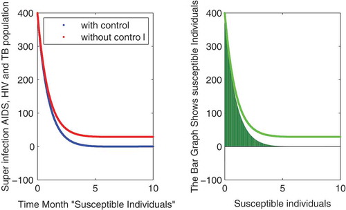
Figure 2. The plot shows the behavior of Latent TB individuals either with and without control.

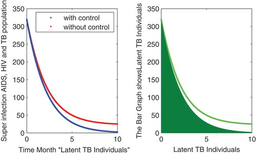
Figure 3. The plot shows the behavior of active TB individuals either with and without control.

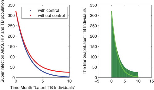
Figure 4. The plot shows the behavior of TB-recovered individuals either with and without control.

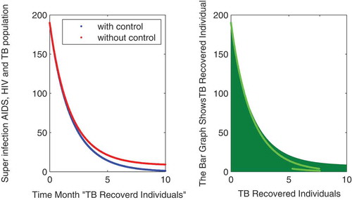
Figure 5. The plot shows the behavior of HIV with no AIDS symptoms in individuals either with and without control.

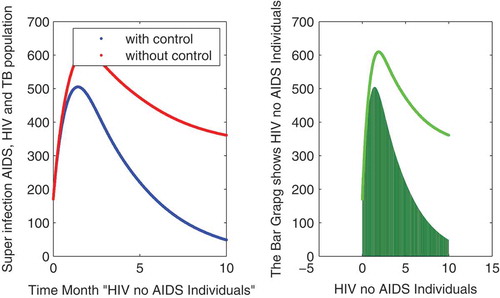
Figure 6. The plot shows the behavior of HIV/AIDS individuals either with and without control.

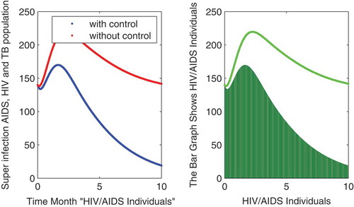
Figure 7. The plot shows the behavior of HIV-infected individuals either with and without control.

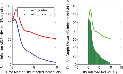
Figure 8. The plot shows the behavior of latent TB/HIV-infected individuals either with and without control.

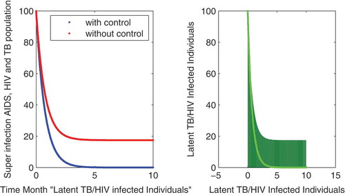
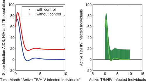
Figure 9. The plot shows the behavior of active TB/HIV-infected individuals either with and without control.

Authors contribution

All authors equally contributed to this paper.

Conflict of Interest

There is no conflict of interest regarding this paper.

Acknowledgements

All authors read and approved the final version.

Additional information

Funding

The authors received no direct funding for this research.

Notes on contributors

Muhammad Tahir

Muhammad Tahir is the corresponding author of this research article. His areas of research are Mathematical Biology and Fluid Dynamics. He is affiliated with Department of Mathematics, Islamia College, University Peshawar, 25000 Pakistan. E-mail: [email protected]; Tel: [phone]

Syed Inayat Ali Shah

Syed Inayat Ali Shah is currently working as a professor and dean in Mathematics at Islamia College University Peshawar, 25000 Pakistan. He has obtained his Ph.D. degree from Saga University, Japan, in 2002. E-mail: [email protected]

Gul Zaman

Gul Zaman is currently working as a vice chancellor at University of Malakand, lower Dir, 18800 Chakdara, Pakistan. He has obtained his Ph.D. from Pusan National University, South Korea, in 2008. E-mail: [email protected]

References

- About HIV/AIDS. (2015, December 6) CDC.
- Basic Statistics. (2015, November 3). CDC.
- Cunningham, A. L., Donaghy, H., Harman, A. N., Kim, M., & Turville, S. G. (2010). Manipulation of dendritic cell function by viruses. Current Opinion in Microbiology, 13(4), 524–17. PMID 20598938. doi:10.1016/j.mib.2010.06.002.
- Doitsh, G., Galloway, N. L. K., Geng, X., Yang, Z., Monroe, K. M., Zepeda, O., … Greene, W. C. (2014). Cell death by pyroptosis drives CD4 T-cell depletion in HIV-1 infection. Nature, 505(7484), 509–514. PMC 4047036?Freely accessible. PMID 24356306. doi:10.1038/nature12940.
- Evian, C. (2006). Primary HIV/AIDS care: A practical guide for primary health care personnel in a clinical and supportive setting. (4th ed, pp. 29). Houghton [South Africa]: Jacana. ISBN 978-1-77009-198-6.
- Fact sheet - Latest statistics on the status of the AIDS epidemic | UNAIDS. www.unaids.org 2017.
- HIV/AIDS Fact sheet N360. WHO. November 2015
- Hu, D. (2001). Radiology of AIDS. Berlin [u.a.]: Springer. pp. 19. ISBN 978-3-540-66510-6.
- International Committee on Taxonomy of Viruses. (2002a). 61.0.6. Lentivirus. National Institutes of Health.
- International Committee on Taxonomy of Viruses. (2002b). 61. Retroviridae. National Institutes of Health.
- Khan, M. A., et al. (2012). Optimal compaign in leptospirosis epidemic model by multiple control variables. Applied Mathematics, 3, 1655–1663. doi:10.4236/am.2012.311229
- Khan, M. A., Zaman, G., Islam, S., & Chohan, M. I. (2013a). Application of homotopy perturbation method to vector host epidemic model with non-linear incidences. Research Journal of Recent Sciences, 2, 90–95.
- Khan, M. A., Islam, S., Ullah, M., Khan, S. A., Zaman, G., Arif, M., & Sadiq, S. F. (2013b). Analytical solution of the leptospirosis epidemic model by homotopy perturbation method. Research Journal of Recent Sciences, 2, 66–71.
- Kumar, V., Abbas, A. K., Fausto, N., & Mitchell, R. N. (2007). Robbins basic pathology (8th ed, pp. 516–522). Saunders Elsevier. ISBN 978-1-4160-2973-1.
- Lawn, S. D., & Zumla, A. I. (2011, July 2). Tuberculosis. Lancet, 378(9785), 57–72. doi:10.1016/S0140-6736(10)62173-3.
- Lenhart, S., & Workman, J. T. (2007). Optimal control applied to biological models, in: Mathematical and computational biology series. London, UK: Champion and Hall, CRC.
- Mandell, B., & Dolan (2010). Chapter 118.
- Markowitz, edited by William N. Rom; associate editor, Steven B. (2007). Environmental and occupational medicine (4th ed.). Philadelphia: Wolters.
- Sweilam, N. H., & Mekhlafi, S. M. A. L. “On the optimal control for fractional multi-strain TB model” 10 March 2016 doi:10.1002/oca.2247.
- Tahir, M., Shah, S. I. A., Zaman, G., & Khan, T. (2018). Prevention strategies for mathematical model MERS-corona virus with stability analysis and optimal control. Journal of Nanoscience and Nanotechnology, 2, 401.
- Tahir, M., & Shah, S. I. A. (0000). A mathematical co-infection problem its transmission and behaviour is presented with stability analysis. SeMA Journal. doi:10.1007/s40324-018-0176-y
- Tahir, M., Shah, S. I. A., & Zaman, G. (2018). Approach for optimal control to prevent infectious diseases from community. Journal of Advanced Physics, 7, 478–486. doi:10.1166/jap.2018.1467
- Tuberculosis. (2002). World Health Organization.
- Tuberculosis Fact sheet N104. (2015, October). WHO.
- UNAIDS, WHO. (2007, December). 2007 AIDS epidemic update (PDF). p. 10 doi:10.1094/PDIS-91-4-0467B
- Win Min, H., Apornpong, T., Kerr, S. J., Hiransuthikul, A., Gatechompol, S., Do, T., Ruxrungtham, K., & Avihingsanon, A. (2018). CD4/CD8 ratio normalization rates and low ratio as prognostic marker for non-AIDS defining events among long-term virologically suppressed people living with HIV. AIDS Research and Therapy. doi:10.1186/s12981-018-0200-4
- WHO. (2007). WHO case definitions of HIV for surveillance and revised clinical staging and immunological classification of HIV-related disease in adults and children. (PDF). Geneva: World Health Organization. pp. 6–16. ISBN 978-92-4-159562-9.
- Zaman, G., Kang, Y. H., & Jung, I. H. (2009). Optimal treatment of an SIR epidemic model with time delay. Biosystems, 98, 43–50. doi:10.1016/j.biosystems.2009.05.006