Optimization of the richardson integration over fluctuations of its step sizes

Abstract

In this paper, we examine the optimization of Richardson numerical integration of an arbitrary real valued function in the space of step sizes. Namely, as one of the most efficient numerical integrations of an integrable function, the Richardson method is optimized under the variations of its step sizes. Subsequently, we classify the stability domains of the Richardson integration of real valued functions. We discuss stability criteria of the Richardson integration via the sign of the fluctuation discriminant as a quintic or lower degree polynomials as a function of the step size parameter. As special cases, our proposal optimizes the trapezoidal, Romberg and other numerical integrations. Hereby, we consider the optimization of the Richardson schemes as a weighted estimation in the light of extrapolation techniques. Finally, optimal Richardson integrations are discussed towards prospective theoretical and experimental applications and their industrial counterparts.

Keywords:

• Optimization theory
• fluctuation theory
• stability analysis
• richardson integration
• numerical techniques

PUBLIC INTEREST STATEMENT

This paper examines the optimization of the Richardson integration of an arbitrary real valued function under variations of its step sizes. Richardson integration is one of the most efficient methods to integrate an integrable function numerically. Our method offers minimized value of the errors under variations of step sizes of the integration. We classify the stability domains of the Richardson integration of arbitrary real valued functions. Subsequently, we discuss stability criteria of the Richardson integration through the sign of the fluctuation discriminant that arises as a quintic polynomial or lower degree polynomials as a function of the step size parameters. As special cases, our proposal optimizes the trapezoidal, Romberg and other numerical integrations. Hereby, we consider the optimization of Richardson schemes as a weighted estimation in the light of extrapolation techniques. Finally, optimal Richardson integrations are discussed towards the prospective theoretical and experimental applications and their industrial counterparts.

1. Introduction

Optimization theory enables an understanding of fluctuation phenomena and their stability properties for a wide class of objective functions and searching algorithms (Parikh & Boyd, 2014). In this paper, we concentrate on optimization of numerical integration techniques over variations of their step sizes, see (Wen, Wang, Jin, Wong, & Ting, 2016) towards the Bayes-optimal joint channel-and-data estimation. Following the fact that the Richardson method incorporates most of the known numerical integration schemes (Chapra & Canale, 1998), we optimize the Richardson estimation of a definite integral of an arbitrary integrable function under variation of its step sizes. In the light of scientific computing (Kincaid, Kincaid, & Cheney, 2009), extrapolation techniques play an important role in trading-off the speed and accuracy of a given numerical integration or a proximal algorithm. In this regard, there are interesting developments towards the fractional calculus (Changpin & Zeng, 2015), critical exponents and series extrapolation techniques for a sequence of data (Cöster & Schmidt, 2016), and associated numerical extrapolation samples (Liu, 2006).

Historically, the Richardson method was found by Lewis Fry Richardson in 1927 who called it as the deferred approach to the limit (Schmidt & Henrici, 1966). This concerned a discrete variable analysis for a system of ordinary differential equations. Further, the Richardson method finds applications in a number of areas of numerical methods, statistical analysis and applied mathematics, see (Schmidt & Henrici, 1966) for analyzing a system of ordinary differential equations, (Little & Rubin, 2014) statistics of missing data, (Hundsdorfer & Verwer, 2013) numerical solution of diffusion equations and (Lambert, 1991) differential systems as initial value problems. As the result, it has become a powerful computational tool (Ouannas & Odibat, 2015), which is massively used in discrete dynamical systems and their evolutions as the initial/boundary value problems. For a system of ordinary differential equations, the Richardson method gives the best approximate solutions with an improved accuracy of the results, see (Ruyer-Quil & Manneville, 2002) for an instance. First of all, for a given real valued function, an extrapolation of the numerical integrations to the limiting zero interval spacing is realized on the basis of algebraic methods (Kappe & Warren, 1989), and associated numerical evaluations and their error analysis (Igoe, 1967). Hereby, it is demonstrated that some numerical evolutions confirm an essential validity towards their optimization procedure (Deb, 2005). In contrast to the above, some of the numerical schemes however show that their extrapolation technique must be used with a caution. As a matter of the fact, the implementation can vary into two types as the active and passive Richardson extrapolations, for an instance, see (Faragó, Havasi, & Zlatev, 2010) towards the stability analysis, optimization algorithms and reliability, (Mona, Lagzi, & Havasi, 2015) towards advection problems, and (Dimov, Zlatev, & Faragó, 2017) for the associated engineering applications and their practical aspects.

In order to reduce the step size, many methods can be used where the higher order terms are considered as the floating points while rounding-off of the errors in a given numerical integration scheme. In this concern, Refs. (Maharani, Salhi, & Suharto, 2018) provide an optimization analysis of floating locations and robust domain determination in the light of the linear system theory and artificial intelligence based algorithm. As an extrapolation model, such problems can be solved by using a weighted average (Liu, 2006), also see (Gao, Sun, & Zhang, 2014) for fractional numerical differentiations as an approximation of the Caputo fractional derivative (Podlubny, 1998) and its applications towards computational studies. Namely, a finite sequence $\{F_n\}$ can be realized as the values of the function $F(h)$. As $h\to 0^{+}$, such an extrapolation model can be expressed (Liu, 2006) as the following asymptotic series

(1) $F(h)=F+\sum _{k=1}^s{\alpha }_k{h}^{p_k}+O(h^{p_s+1}),$(1)

where the first term F is understood as the limit $F=li{m}_{h\to 0}F(h),{\alpha }_k$ are constants that are independent of the step size $h$, and the exponents $\{p_k\}$ satisfy $p_1<p_2<\cdots <p_{s+1}$.

In this concern, the Richardson extrapolation arises as a type of numerical differentiations that includes highly accurate finite difference formulae and reduces various errors (Chapra & Canale, 1998; Keller, 2018; Liu, 2006). In order to get an accurate approximation, we offer the optimal Richardson method that combines various numerical integral estimates such as the trapezium, Simpsons and Romberg techniques (Chapra & Canale, 1998). As a special case of the Richardson integration scheme, the Romberg method arises as an initial value theory (Bauer, Rutishauser, & Stiefel, 1963), whereupon various numerical and computational aspects are established in the light of numerical integrations of an integrable real valued function (Samoradnitsky, 2017). In early time analysis, such evolutions correspond to stable non-Gaussian random processes (Lambers & Sumner, 2016).

Fluctuation theory finds its relations to the stochastic modelling, dynamical systems, recurring events, control systems and queuing theory (Asmussen & Albrecher, 2010). In this regard, there exists a concrete formula (Feller, 2015) for stable distributions and its applications to Markov chains and their ergodic properties. As per this introduction, we consider fluctuations of the Richardson numerical integration of an arbitrary real valued function in the space of step sizes. In practice, fluctuations introduce some fuzziness in the parameters, whereby they are measured probabilistically, see (Zimmermann, 1975) towards the optimization of fuzzy systems. Fluctuation theory has an intrinsic geometric origin, see (Ruppeiner, 1995) for a Riemannian geometric description of thermodynamic fluctuations, and (Tiwari, 2008) for its relation to black objects and their geometric invariants at different orders of perturbations. Indeed, fluctuations are closely intertwined with optimization theory, see for instance (Xie, Zhang, & Yang, 2002) towards the particle swarm optimization, evolutionary computing and dissipative models and (Harkey & Kenny, 2000) for conductance fluctuations (termed as $1/f$ noise) in microelectromechanical systems. System optimizations have their deep-rooted origin in the theory of estimation, for example, the second-order homogenization estimates (Castan˜eda, 2002) as well as in the theory of computing and information science, see (Saitou, Izui, Nishiwaki, & Papalambros, 2005) towards product developments and structural optimization techniques. Furthermore, it is worth mentioning that the fluctuation theory analysis plays an important role in examining the Brownian motion of a particle moving in a periodic potential (Bao-Quan et al., 2003) and associated numerical integral, also see (Hairer, Lubich, & Wanner, 2006) towards its geometric description, structure-preserving algorithms and numerical solutions of a system of ordinary differential equations.

In the light of embedded systems, our model does not stop here, but it finds its perspectives in the realm of computational methods, Monte Carlo simulations, random processors, viz. Gaussian and non-Gaussian configurations (Hairer et al., 2006). With this motivation, we focus on the stability structures of an arbitrary embedded system and its flow analysis, see (Tiwari, 2011a) in the light of convexity theory and its geometric perspectives. Perspectives of fluctuation theory include dynamic optical optimization (Kuipo et al., 2016), multicomponent constrained optimizations (Tiwari, Kuipo, Bellucci, & Marina, 2016), power networks and their geometric stability analysis (Bellucci, Tiwari, & Gupta, 2012). Further engineering developments exist, see (Gupta, Tiwari, & Bellucci, 2013) towards an intrinsic geometric understating of the network reliability and voltage stability towards the optimal solution of power system planning and its operation. Such problems are highly nonlinear and large-scale in their nature. Notice that fluctuation theorems arise as a consequence of the time reversal symmetry, and symmetries of the hyperbolic spaces and transitive maps. Namely, such a theorem provides asymptotic observations in time. In the framework of approximation theory, a quantitative and parameter free relation between the stationary probabilities of observing a value emerges as the average entropy production rate and vice-versa. Further interests include its connections towards the chaotic hypothesis and chaotic dynamical systems (Ott, 2002).

Consequently, as per the above notion of the system reliability, optimizations of such systems as a state model yield different thermodynamic properties (Kozioł & Wiśniewski, 2008), see (Angelis, 1994) also towards a variation theory investigation and (Lei, Chengjun, & Chen, 2018) for associated flow properties in the space of parameters. In this paper, as far as the stability of the Richardson scheme is concerned, we find that the fluctuation discriminant arises as a quintic equation in the step size parameter, whereby we discuss the statistical nature of the undermining ensemble both in general and various limiting cases. This offers an intriguing relationship with fundamental objects in the algebraic theory of equations [47]. For example, finite degree rational curves show an interesting property in relation to compact Calabi-Yau three-folds (Candelas, Xenia, Green, & Parkes, 1991) and their moduli spaces that can be viewed as a discrete finite set, that is, a rational curve of its highest degree nine (Johnsen & Kleiman, 1996) or that of a curve of it degree eleven (Cotterill, 2012) on a generic quintic 3-fold. In this regard, the associated Donaldson-Thomas invariants render interesting platforms to study algebraic equations and rational curves in the light of the algebraic geometry (Clemens, 1984), Picard-Fuchs equations and mirror maps (Cox & Katz, 1999).

Dynamics of nonlinear configurations possess non-integrable and asymptotic characteristics. In general, such systems cannot be solved by using an analytic method. Therefore, numerical perturbation and reduction techniques are used to optimize the evolution of such systems as a function of the time. For example, the Hamilton-Jacobi-Bellman equation is one approach that optimizes such nonlinear systems (Clarkson, 1993). This offers an intrinsic interrelation of the optimization theory to nonlinear dynamical systems and associated geometric methods. Furthermore, as a nonlinear system, nonlinear adaptive controls enable us to identify the unknown parameters of the model (Marino, 1997). As a stabilization problem, the uncertainties can enter via either the state or input variables of a given system as a pair of dual variables, such as the co-ordinate and momentum or the energy and time, see (Tiwari, 2011b) towards generalized uncertainty principles and their relation to physical systems. In the light of the control theory, a complete set of solutions are known for certain limiting quadratic systems (Khargonekar, Petersen, & Zhou, 1990). Such robust stabilization problems exist in the realm of the control theory (Khargonekar et al., 1990) and stochastic models (Kushner, 1967).

Notice that considerations concerning the Richardson integration that focus on the optimization of coefficients in Romberg-like algorithms are of a fundamental importance, see for instance the classic book by Store and Bulirsch (Stoer & Bulirsch, 2013) for an overview of the literature. In this concern, there exist a number of computational analysis (Kiusalaas, 2013) in the light of the Romberg integration scheme and extrapolation methods for a smooth nonperiodic function. However, as far as the convergence of the solution $f$ of an ordinary differential equation is concerned, it is worth mentioning that the existing Romberg quadratures do not provide an improvement(Ciarlet, 2001), when the derivative of $f$ is discontinuous at certain point(s) in the solution space. The optimization of such solutions and their application arise in diverse engineering and system designing problems. Following the same, we have provided an intrinsic classification scheme and computed stability properties of the Richardson integration of an arbitrary real valued smooth function in terms of algebraic relations, namely, as the polynomials in the step-size parameter. As an innovation in the optimization theory, our proposal offers stable solutions of ordinary differential equations that are function independent in their nature. Hereby, the above proposed scheme finds its importance in engineering applications and interdisciplinary research. With this motivation, we explore the optimization of an arbitrary Richardson integral as a weighted extrapolation model, see (Cabrera & Parks, 1991) towards the understanding of spectral estimation techniques, data analysis and signal processing.

In this paper, we give the optimal Richardson integration of a real valued function under variations of its step sizes. Namely, we have provided the optimization of the Richardson numerical integration in the space of its step sizes. Herewith, about its critical points, we find that the flow components defined as the first order partial derivative of the integration have the same ratio as that of the step sizes. For a given real smooth function, we have shown that the critical points of the Richardson numerical integration are expressible as a function of the flow components. In this setting, the critical points of the Richardson integration arise as the roots of the corresponding flow equations. As a function of the step sizes, this results into a set of algebraic equations that need to be simultaneously solved in order to get the critical points. Hereby, we have obtained all possible critical points of the Richardson numerical integration of an arbitrary integrable real valued function. Further, in the limit of small step sizes, it is shown that the origin emerges as a repeated root of the flow equations. Apart from the origin, we find that there is a nontrivial repeated root along with two other simple roots. In the squeal, we have computed the fluctuation capacities as the pure second order partial derivatives of the Richardson numerical integration of an arbitrary real valued smooth function. In addition, we have calculated the undermining correlation between the step sizes as its mixed second order partial derivative. At a given critical point, the global stability of the Richardson numerical integration is governed by the sign of the discriminant. It is explicitly shown that the numerator of the discriminant arises as a fifth order polynomial in the step size parameter.

With the above motivation, the rest of the paper reads as follows. In section 2, we provide a brief review of the model and give highlights of the Richardson method by invoking the role of the trapezium rule. In the sequel, we discuss the Romberg method as a special case of the Richardson numerical integration. In section 3, considering the fact that the Richardson integration depends on a pair of step sizes, we give an overview of the stability analysis of a two variable function in the space of step sizes. In section 4, we optimize the Richardson integration under fluctuations of its step sizes and depict the system stability via a degree five polynomial in the square of the ratio of the step sizes around the unity. Hereby, we obtain all possible critical points of the Richardson numerical integration of arbitrary integrable function. In section 5, following the above results as in the section 4, we discuss stability criteria for the Richardson integration scheme in various limiting cases. In order to assimilate the stability structures of the Richardson integration, we offer the flowchart of our analysis, discuss various limiting cases to characterize the stability of the Richardson numerical integration of an arbitrary real valued function and provide summary of the concerned results in a tabular format. In section 6, we offer a qualitative discussion of the Richardson theory with the existing models that are commonly explored in the light of system optimizations, fluids engineering, business media and fast sea transportation. Hereby, perspective applications are anticipated in the domain of the sensitivity analysis, finite difference schemes, and non-uniform grids. In reference to the original Richardson’s dream towards the atmospheric circulation and forecasting of the weather as a time integration, our study supports modeling of discrete dynamical systems, numerical simulations, system engineering and computational mechanics. Finally, in section 7, we conclude the paper with a brief summary and perspective directions for future research and developments.

2. Review of the model

In this section, we provide a brief review of the Richardson integration of an arbitrary real valued function. Considering a numerical method that performs the integration of a real valued function $F(x)$ on a computer or a machine, it is known (Battaglia et al., 2015) that the accuracy depends on the step size $h$ as in Eqn. (1). In practice, it follows that when the estimated value of a numerical integral tends to its true value, the step size of the integration tends to zero (Battaglia et al., 2015). In this case, let $p^{\star }$ be the order of the accuracy, then using step size $h$, it is known (Battaglia et al., 2015) that the function $F(h)$ can be expressed as the following approximation

(2) $F(h)={\alpha }_0+{\alpha }_1{h}^{p^{\star }}+O(h^r),r>p^{\star }.$(2)

Here, the true value of $F$ is found as the $0^{th}$ order coefficient

(3) $F(0)={\alpha }_0.$(3)

In this case, the exact value $\mathbb{I}$ of the integral of the function $F$ in the trapezoidal rule (Battaglia et al., 2015), the estimated value $I(h)$ and the associated true error $E(h)$ (Kaw & Krivanek, 2018) can be represented as

(4) $\mathbb{I}=I(h)+E(h).$(4)

Notice that the step size $h$ of the integral $\mathbb{I}$ can be obtained from its limits and the number of steps. Namely, if the integral is performed from $a$ to $b$ in $n$ steps, then the step size $h$ is given by $(b-a)/n$. For example, the integration $I(h)$ is realized as an estimated value of $\mathbb{I}$ and $E(h)$, that is, the true error for $I(h)$. To be precise, if we consider two different step sizes $\{h_1,h_2\}$, then the true errors $\{E(h_1),E(h_2)\}$ and the respective estimated values $\{I(h_1),I(h_2)\}$ may vary, however, the exact value of $\mathbb{I}$ remains the same, see (Chapra & Canale, 1998) for an instance. Herewith, from Eqn. (4), it follows that we have the equality

(5) $I(h_1)+E(h_1)=I(h_2)+E(h_2).$(5)

In the numerical analysis, it is known (Chapra & Canale, 1998) that the true error in the trapezoidal integration of an arbitrary real valued function $F$ is given by

(6) $E(h)\cong -\frac{b-a}{12}{h}^2{\bar{f}}^{\prime \prime }.$(6)

Assuming that the second derivate ${\bar{f}}^{\prime \prime }$ evaluated at a given point is a constant, it follows from Eqn. (6) that the respective errors $E(h_1)$ and $E(h_2)$ corresponding to the step sizes $h_1$ and $h_2$ satisfy

(7) $E(h_1)\cong E(h_2){\left(\frac{h_1}{h_2}\right)}^2.$(7)

Substituting Eqn. (7) into Eqn. (5), we get the following estimation of the subsequent error

(8) $E(h_2)\cong \frac{I(h_2)-I(h_1)}{{\left(\frac{h_1}{h_2}\right)}^2-1}.$(8)

From Eqns. (4, 8), it follows that the integral $\mathbb{I}$ can be expressed as

(9) $\mathbb{I}(h_1,h_2)\cong I(h_2)+\frac{I(h_2)-I(h_1)}{{\left(\frac{h_1}{h_2}\right)}^2-1}.$(9)

Hereby, we see that the integral $\mathbb{I}$ can be expressed solely as a function of the step sizes $\{h_1,h_2\}$. In this paper, our motivation is to find the optimal value of $\mathbb{I}$ as in the above Eqn. (9). Further, as a special case, our method incorporates optimization of the trapezium integration and Romberg method, see (Chapra & Canale, 1998) for detail. Namely, from Eqn. (9), this is performed as a weighted estimation using $h_2=h_1/2$ as

(10) $\mathbb{I}\approx \frac{4}{3}I(h_2)-\frac{1}{3}I(h_1).$(10)

In particular, Eqn. (10) offers an estimate of the trapezoidal scheme when the step sizes are repeatedly halved, see (Chapra & Canale, 1998) for an introduction. Moreover, in the light of the extrapolation theory (Battaglia et al., 2015), we get the Romberg Integration as the following recursion equation

(11) $I_{j,k}\approx \frac{4^{k-1}{I}_{j+1,k-1}-I_{j,k-1}}{4^{k-1}-1},$(11)

where $j,k=1,2,\dots ,N$ with $N$ as the number of step sizes used to evaluate a given definite Richardson integral. Herewith, the Richardson method incorporates the Romberg extrapolation methods, wherefore our method inherits an intrinsic optimization of the Richardson extrapolation techniques.

With the above motivations, we consider the optimization of well-known Richardson integration with respect to the choice of the consecutive step sizes. Here, from the perspective of the intrinsic fluctuations, the objective function in our approach is to optimize the Richardson integration of an arbitrary real valued function $F$ in the space of its step sizes. In particular, in this formulation, the task proposed is realized by combining different parts of the integral that is defined as a definite integral of the type $\mathbb{I}={\int }_a^{b}F(x)dx$ that is sought to be computed numerically.

In this paper, one of the main motivations is to find the optimal value of the above $\mathbb{I}$. Notice that $\mathbb{I}$ attains a fixed value when it is performed in the continuous way, that is, when there is no error. In the other words, when $\mathbb{I}$ is not evaluated by a numerical integration method, then there is nothing to be optimized. However, when the integration $\mathbb{I}$ is performed numerically, one deals with the quadrature formula. Therefore, the obtained numerical value of $\mathbb{I}$ needs to be optimized, that is, the exact error $\mathbb{E}$ governing the precision of $\mathbb{I}$ that depends on certain parameters should be minimized. In this setting, these parameters are considered as the consecutive step sizes that are used in the numerical evaluation of $\mathbb{I}$ satisfying

(12) $\mathbb{I}-I(h_2)-\frac{I(h_2)-I(h_1)}{{\left(\frac{h_1}{h_2}\right)}^2-1}=\mathbb{E}$(12)

From the above Eqns. (9, 12), it follows that in the limit of the quadrature formula (Battaglia et al., 2015), the optimization of $\mathbb{I}$ is the same as the minimization of the above exact error $\mathbb{E}$. In this sense, for a given $F$ as above, we optimize the Richardson integration $\mathbb{I}$ in the space of execution parameters $\{h_1,h_2\}$, as depicted above in the Eqn. (9).

Following the same, we discuss the critical points of the quadrature formula, which is considered as a function of the two step sizes $\{h_1,h_2\}$. In the light of numerical practices, the significance of the results of this discussion is that it gives the optimal value of the Richardson integration of a smooth real valued function when it is performed by a machine of finite memory storage capacity. To be precise, for a given $f$ whose Richardson integration $\mathbb{I}$ is to be numerically computed on a given machine of finite memory capacity $n$, the inverse of $n$ can be used to define the error of an evaluation of the Richardson integration $\mathbb{I}$. Hereby, in the light of numerical practices our scheme offers an intrinsic computational significance that is equally supported by a machine. In this direction, numerical tests of the proposed approach as well as its comparison with other quadrature methods are among the promising directions that we leave open for prospective research and developments. In particular, the practical effects of the proposed optimization scheme are anticipated to be demonstrated in the future.

In nutshell, our proposal gives an intrinsic methodology to determine the optimal values of the Richardson integration of a smooth real valued function when it is numerically performed by a machine with its initial and final step size $h_1$ and $h_2$. In addition, the condition that the quantities $\{(b-a)/h_j|j=1,2,\dots ,N\}$ should be natural numbers is considered in the light of derandomization theory, see (Agrawal & Biswas, 2003) for an introduction. Namely, in a de-randomized system based formulation of the optimization task, these would emerge as the integer valued numerical constraints. Herewith, for a given sequence of step-sizes $\{h_i|i=1,2,\dots ,N\}$, both step sizes are anticipated to give correct partitions of the integration interval $(a,b)$ up to a computational error, that is, we have step-size spacing $h_{i+1}-h_i$ in the sense of the forward difference and that of $h_i-h_{i-1}$ in the sense of the backward difference in the light of numerical studies.

3. Step size fluctuations

In this section, we provide an overview of the fluctuation theory in the light of the Richardson numerical integration as defined above in Eqn. (9). Considering the step sizes $h_1$ and $h_2$ of the integration of $F$ as the fluctuation parameters, we examine stability properties of the statistical system by considering the Richardson integration $\mathbb{I}(h_1,h_2)$ as the embedding function over the surface of step sizes $\{h_1,h_2\}$. Namely, we have explained the nature of the embedding map from the space of step sizes $h_1$ and $h_2$ to the set of real numbers, its critical points whether they correspond to a minimum, maximum or a saddle point and discuss the convergence of the Richardson integral $\mathbb{I}(h_1,h_2)$ of $F$ to its true value. To be precise, given the two embedding variables as the step sizes $(h_1,h_2)\in {\mathcal{M}}^2$, the behavior of the integral $\mathbb{I}(h_1,h_2)$ about its critical points $(h_1^0,h_2^0)$ can be determined by the Taylor series expansion

(13) $\begin{array}{cc}\mathbb{I}(h_1,h_2)=& \mathbb{I}(h_1^0,h_2^0)+{\mathbb{I}}_1(h_1,h_2)(h_1-h_1^0)+{\mathbb{I}}_2(h_1,h_2)(h_2-h_2^0)\\ \hspace{0.17em}& +\frac{1}{2!}{\mathbb{I}}_{11}(h_1,h_2)(h_1-h_1^0{)}^2+\frac{1}{2!}{\mathbb{I}}_{22}(h_1,h_2)(h_2-h_2^0{)}^2\\ \hspace{0.17em}& +{\mathbb{I}}_{12}(h_1,h_2)(h_1-h_1^0)(h_2-h_2^0)+\cdots ,\end{array}$(13)

where the symbols $\{{\mathbb{I}}_1(h_1,h_2),{\mathbb{I}}_2(h_1,h_2)\}$ denote the first order partial derivatives of $\mathbb{I}(h_1,h_2)$ and $\{{\mathbb{I}}_{11}(h_1,h_2),{\mathbb{I}}_{22}(h_1,h_2),{\mathbb{I}}_{12}(h_1,h_2)\}$ are its second order partial derivatives evaluated at a critical point. About a given critical point $(h_1^0,h_2^0)$ as roots of the flow equations ${\mathbb{I}}_1(h_1,h_2)=0$ and ${\mathbb{I}}_2(h_1,h_2)=0$, then up to the second order terms, the above Taylor series as in Eqn. (13) can be expressed as the below quadratic curve

(14) $\begin{array}{c}\mathbb{I}(h_1,h_2)=a+b{(h_1-h_1^0)}^2+c{(h_2-h_2^0)}^2+d(h_1-h_1^0)(h_2-h_2^0),\end{array}$(14)

in $h_1$ and $h_2$. Here, the expansion coefficients $\{a,b,c,d\}$ are defined as $a=\mathbb{I}(h_1^0,h_2^0)$, $b={\mathbb{I}}_{11}(h_1^0,h_2^0)/2$, $c={\mathbb{I}}_{22}(h_1^0,h_2^0)/2$, and $d={\mathbb{I}}_{12}(h_1^0,h_2^0)$. In order to find the roots $(h_1^0,h_2^0)$, the partial derivatives $\{{\mathbb{I}}_1(h_1,h_2),{\mathbb{I}}_2(h_1,h_2)\}$ with respect to $h_1$ and $h_2$ of the integral $\mathbb{I}(h_1,h_2)$ should be equated to zero, that is, we are required to simultaneously solve the equations ${\mathbb{I}}_1(h_1,h_2)=0$ and ${\mathbb{I}}_2(h_1,h_2)=0$. To be precise, let the solutions of the above equations be $h_1=h_1^0$ and $h_2=h_2^0$, then the critical point of $\mathbb{I}(h_1,h_2)$ arises as a pair $(h_1^0,h_2^0)$. In order to check the behavior of a critical point, we need to find the signature of discriminant

(15) $\mathrm{\Delta }={\mathbb{I}}_{11}(h_1,h_2){\mathbb{I}}_{22}(h_1,h_2)-{\mathbb{I}}_{12}(h_1,h_2{)}^2.$(15)

Physically, the behavior of a critical point $(h_1^0,h_2^0)$ is summarized as per the following criteria

1. If $\mathrm{\Delta }<0$ at $(h_1^0,h_2^0)$, then the critical point $(h_1^0,h_2^0)$ is a saddle point of $\mathbb{I}(h_1,h_2)$.

2. If ${d_1}^4<-n_0/n_4$ at ${\mathrm{\Delta }}_2<0$, then we have the following classification.

   1. If either ${\mathbb{I}}_{11}(h_1,h_2)$ or ${\mathbb{I}}_{22}(h_1,h_2)<0$ at $(h_1^0,h_2^0)$, then $(h_1^0,h_2^0)$ is the maximum of $\mathbb{I}(h_1,h_2)$.

   2. If either ${\mathbb{I}}_{11}(h_1,h_2)$ or ${\mathbb{I}}_{22}(h_1,h_2)>0$ at $(h_1^0,h_2^0)$, then $(h_1^0,h_2^0)$ is the minimum of $\mathbb{I}(h_1,h_2)$.

   3. If either ${\mathbb{I}}_{11}(h_1,h_2)$= 0 or ${\mathbb{I}}_{22}(h_1,h_2)=0$ at $(h_1^0,h_2^0)$, then $(h_1^0,h_2^0)$ corresponds to neither a maximum nor a minimum of $\mathbb{I}(h_1,h_2)$.

3. If $\mathrm{\Delta }=0$ at $(h_1^0,h_2^0)$, then the test fails and we say that the function $\mathbb{I}(h_1,h_2)$ is too flat. Therefore, we need a higher derivative test in order to examine the stability properties of $\mathbb{I}(h_1,h_2)$ under fluctuations of its step sizes $\{h_1,h_2\}$ for a chosen Richardson numerical integration.

In this regard, the aim is to optimize the Richardson integration $\mathbb{I}$ of an arbitrary integrable function under variations of its step sizes $\{h_1,h_2\}$. In the next section, as $\{h_1,h_2\}$ vary, we study fluctuations of the Richardson integration $\mathbb{I}(h_1,h_2)$ about is critical points $(h_1^0,h_2^0)$. Hereby, the integration $\mathbb{I}$ reaches a fixed value when $h_1$ and $h_2$ are taken at their critical values $(h_1^0,h_2^0)$. This follows from the aforementioned fact that the numerical computation of a definite integral possesses an exact error. Further, the optimization of $\mathbb{I}$ is in correspondence with the optimization the exact error $\mathbb{E}$. Moreover, up to a given nonzero maximum error $e=max\{\mathbb{E}\}$, from Eqn. (12), it follows that the extrimization of $\mathbb{I}$ is equivalent to the extrimization of the exact error $\mathbb{E}$. In the light of numerical practices, as a function of the step size parameter, the significance of the results is that our analysis gives a quintic type stability criterion as far as the optimization of the Richardson integration of an arbitrary integrable function is concerned under variations of its step sizes, see Eqn. (36) below.

4. Optimal Richardson schemes

In this section, we provide optimization properties of the Richardson integration $\mathbb{I}(h_1,h_2)$ of an arbitrary real valued function $F$ with the integral $I(h_2)$ when it is evaluated at the step size $h_2$ and the integral $I(h_1)$ at that of the step size $h_1$. In order to simplify the calculations, let us define $d_1$ and $d_2$ as

(16) $d_1(h_1,h_2)={\left(\frac{h_1}{h_2}\right)}^2-1,$(16)

(17) $d_2(h_1,h_2)=I(h_2)-I(h_1).$(17)

With the above notations, the Richardson integration as in Eqn. (9) reads as the following function

(18) $\mathbb{I}(h_1,h_2)=I(h_2)+\frac{d_2(h_1,h_2)}{d_1(h_1,h_2)}.$(18)

Hereby, the first order partial derivatives of the function $\mathbb{I}(h_1,h_2)$ with respect to the step sizes $h_1$ and $h_2$ give the flow components of $\mathbb{I}(h_1,h_2)$. For a given pair of $\{d_1,d_2\}$, the derivation of the Richardson integration $\mathbb{I}(h_1,h_2)$ give the flow components $\{{\mathbb{I}}_1(h_1,h_2),{\mathbb{I}}_2(h_1,h_2)\}$. Namely, we notice that the differentiation of $\mathbb{I}(h_1,h_2)$ with respect to $h_1$ results into the following expression

(19) ${\mathbb{I}}_1(h_1,h_2)=-\frac{1}{{d_1}^2}\left(d_1{I}_1(h_1)+\frac{2h_1}{{h_2}^2}{d}_2\right).$(19)

Similarly, by differentiating $\mathbb{I}(h_1,h_2)$ with respect to $h_2$, we find the associated flow component as

(20) ${\mathbb{I}}_2(h_1,h_2)=I_2(h_2)+\frac{1}{{d_1}^2}\left(d_1{I}_2(h_2)+\frac{2{h_1}^2}{{h_2}^3}{d}_2\right).$(20)

Differentiations of the above Eqns. (19, 20) with respect to $h_1$ and $h_2$ give the respective fluctuation capacities that are define as the second order pure partial derivatives $\{{\mathbb{I}}_{11}(h_1,h_2),{\mathbb{I}}_{22}(h_1,h_2)\}$. In order to simplify the notations, we express the fluctuation capacities $\{{\mathbb{I}}_{11}(h_1,h_2),{\mathbb{I}}_{22}(h_1,h_2)\}$ as the function of $d_1$. Differentiating Eqn. (19) with respect to $h_1$, we find the following $h_1$ fluctuation capacity

(21) ${\mathbb{I}}_{11}(h_1,h_2)=\frac{1}{{d_1}^3}(-a_1{d_1}^2+b_1{d}_1-c_1),$(21)

where the coefficients $\{a_1,b_1,c_1\}$ are given by

(22) $a_1=I_{11}(h_1),b_1=\frac{4h_1}{{h_2}^2}{I}_1(h_1)-\frac{2}{{h_2}^2}{d}_2,c_1=\frac{8{h_1}^2}{{h_2}^4}{d}_2.$(22)

Similarly, by differentiating Eqn. (20) with respect to $h_2$, we get the $h_2$ fluctuation capacity as

(23) ${\mathbb{I}}_{22}(h_1,h_2)=\frac{1}{{d_1}^3}(a_2{d_1}^3+a_2{d_1}^2+b_2{d}_1+c_2),$(23)

where the coefficients $\{a_2,b_2,c_2\}$ are given by the expressions

(24) $a_2=I_{22}(h_2),b_2=\frac{4{h_1}^2}{{h_2}^3}{I}_2(h_2)-\frac{6{h_1}^2}{{h_2}^4}{d}_2,c_2=\frac{8{h_1}^4}{{h_2}^6}{d}_2.$(24)

For the above Richardson integration as in Eqn. (18), the correlation between step sizes $h_1$ and $h_2$ is defined by the mixed partial derivative of $\mathbb{I}$. In this case, by differentiating Eqn. (19) with respect to $h_2$, as the function of $d_1$, we find that the correlation ${\mathbb{I}}_{12}$ arises as the following relation

(25) ${\mathbb{I}}_{12}(h_1,h_2)=\frac{1}{d_1^3}(a_3{d_1}^2-b_3{d}_1-c_3),$(25)

where the coefficients $\{a_3,b_3,c_3\}$ read as

(26) $\begin{array}{c}{a}_3=0,\\ b_3=\frac{2h_1}{{h_2}^2}{I}_2(h_2)+\frac{4{h_1}^2}{{h_2}^3}{I}_1(h_1)-\frac{4h_1}{{h_2}^3}{d}_2,\\ c_3=\frac{8{h_1}^3}{{h_2}^5}{d}_2.\end{array}$(26)

In this setting, the critical points of the Richardson numerical integration are given as roots of ${\mathbb{I}}_1(h_1,h_2)$ and ${\mathbb{I}}_2(h_1,h_2)$. Therefore, we are required to simultaneously solve the flow equations: ${\mathbb{I}}_1(h_1,h_2)=0$ and ${\mathbb{I}}_2(h_1,h_2)=0$. From the above Eqn. (19), we see that ${\mathbb{I}}_1(h_1,h_2)=0$ yields

(27) $I_1(h_1)({h_1}^2-{h_2}^2)=-2h_1{d}_2.$(27)

Similarly, the other flow equation ${\mathbb{I}}_2(h_1,h_2)=0$ as in Eqn. (20) gives the following equalities

(28) $h_1=0or{I}_2(h_2)({h_1}^2-{h_2}^2)=-2h_2{d}_2.$(28)

For two distinct step sizes $h_1\ne h_2$ and integral values $I(h_1)\ne I(h_2)$, by dividing Eqn. (27) by (28), we see that the step sizes $\{h_1,h_2\}$ satisfy the following ratio

(29) $\frac{h_1}{h_2}=\frac{I_1(h_1)}{I_2(h_2)}.$(29)

Therefore, we see that the ratio of step sizes $\{h_1,h_2\}$ arises as the ratio of the first derivatives $\{I_1(h_1),I_2(h_2)\}$ at a critical point of $\mathbb{I}$. This defines the equilibrium condition of the Richardson integration when $\{h_1,h_2\}$ vary. Squaring both side of Eqn. (29) and substituting the corresponding value of $h_2$ into Eqn. (27), we get the following values

(30) $h_1=0\mathrm{o}\mathrm{r}{h}_1=h_1^0=\frac{2I_1(h_1)d_2}{I_2{(h_2)}^2-I_1{(h_1)}^2}.$(30)

Substituting the above value of $h_1$ as in Eqn. (30) into Eqn. (28), we find that $h_2$ reads as follows

(31) $h_2=0\mathrm{o}\mathrm{r}{h}_2={h_2}^0=\frac{2I_2(h_2)d_2}{I_2{(h_2)}^2-I_1{(h_1)}^2}.$(31)

In order to get all the solutions of the equations ${\mathbb{I}}_1(h_1,h_2)=0$ and ${\mathbb{I}}_2(h_1,h_2)=0$, for example, in the limit of $h_1\to h_2$, we need to directly solve the above Eqns. (27, 28). In this case, we may directly substitute Eqn. (30) into Eqn. (27) and obtain the corresponding value of $h_2$. By doing so, we find the following values $h_2=\pm {h_2}^0$. Therefore, the possible nontrivial roots are $({h_1}^0,{h_2}^0)$ and $({h_1}^0,-{h_2}^0)$. Similarly, if we use $h_2={h_2}^0$ in Eqn. (28), we get $h_1=\pm {h_1}^0$. Thus, the possible nontrivial roots are $({h_1}^0,{h_2}^0)$ and $(-h_1^0,h_2^0)$. In short, we find that the set of critical points $\mathrm{\Re }$ of $\mathbb{I}$ reads as

(32) $\begin{array}{cc}\mathrm{\Re }=& \{(0,0),(0,0),(h_1^0,h_2^0),(h_1^0,-h_2^0),(h_1^0,h_2^0),(-h_1^0,h_2^0)\}.\end{array}$(32)

In order to study the stability analysis of the Richardson numerical integration, let us consider a critical point $(h_1^i,h_2^i)\in \mathrm{\Re }$. Then, the type of fluctuations about the critical point $(h_1^i,h_2^i)$ is governed by the sign of the discriminant as in Eqn. (15). Substituting the value of fluctuation capacities $\{{\mathbb{I}}_{11},{\mathbb{I}}_{22}\}$ as in Eqns. (21, 23), and the local correlation ${\mathbb{I}}_{12}$ as in Eqn. (25), it is not difficult to show that the discriminant $\mathrm{\Delta }$ reading as

(33) $\begin{array}{cc}\mathrm{\Delta }=& \frac{1}{{d_1}^6}(-a_1{d_1}^2+b_1{d}_1-c_1)(a_2{d_1}^3+a_2{d_1}^2+b_2{d}_1+c_2)-\frac{1}{{d_1}^3}{(a_3{d_1}^2-b_3{d}_1-c_3)}^2,\end{array}$(33)

can be expressed as per the following ratio

(34) $\mathrm{\Delta }=\frac{1}{d_1^6}\sum _{i=0}^5{n}_i{d_1}^i.$(34)

Here, the factors $\{n_i|i=0,1,2,3,4,5\}$ as in Eqn. (34) are defined as

(35) $\begin{array}{cc}{n}_0=& -(c_1{c}_2+{c_3}^2),\\ n_1=& b_1{c}_2-b_2{c}_1-2b_3{c}_3,\\ n_2=& b_1{b}_2-a_1{c}_2-a_2{c}_1-{b_3}^2,\\ n_3=& b_1{a}_2-a_1{b}_2-c_1{a}_2,\\ n_4=& a_2(b_1-a_1),\\ n_5=& -a_1{a}_2.\end{array}$(35)

From Eqn. (34), as a function of the step size parameter $d_1$, it follows that the global stability of the Richardson integration of an arbitrary real valued function $F$ is governed by the sign of the above quintic polynomial

(36) $n(d_1):=\sum _{i=0}^5{n}_i{d_1}^i.$(36)

Namely, in the step size parameter $d_1$, the roots of the above quintic polynomial $n(d_1)$ as in Eqn. (36) satisfy the quintic equation $n(d_1)=0$. Here, as an algebraic polynomial, $n(d_1)=0$ as in Eqn. (36) can be factorized by using Galois theory (Artin, 2007). One can solve such an algebraic equation $n(d_1)=0$ when it is a degree five or reducible to lower degree equations, see (Kappe & Warren, 1989) for an introduction. In the sequel, we provide an explicit analysis of the stability of the Richardson integration of an arbitrary real valued function $F$ under fluctuations of the step sizes $h_1$ and $h_2$. In particular, in the next section, the stable configurations are categorized under various values of the model parameters $\{n_i|i=0,1,2,3,4,5\}$.

5. Discussion of the results

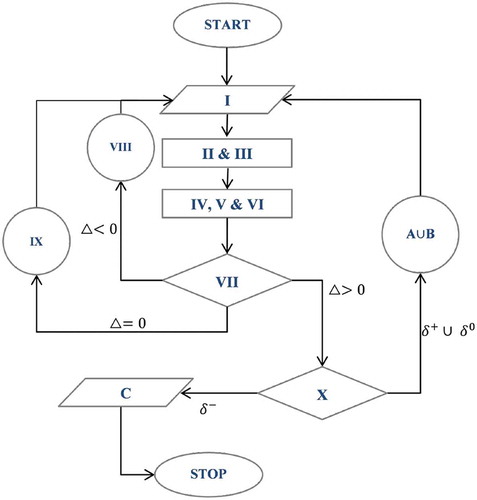
In this section, we provide a flow chart towards the classification of stability criteria of the Richardson numerical integration scheme and its limiting configurations under various cases of the modal parameters $\{n_i|i=0,1,2,3,4,5\}$. To offer a step by step picture of the same, we give the flowchart, discussion of special cases and summary of the results concerning the stability of the Richardson numerical integration of an arbitrary real valued function.

5.1. A flowchart of the stability analysis

To be precise, for the aforementioned Richardson numerical integration of an arbitrary real valued function, let us define the associated quantities as below:

1. Choose the step sizes $h_1,h_2\in \mathbb{R}$ for a given $I:\mathbb{R}\to \mathbb{R}$.

2. Define $d_1=(\frac{h_1}{h_2}{)}^2-1$ and $d_2=I(h_2)-I(h_1)$.

3. Find the critical points $(h_1^0,h_2^0)$ as the roots of ${\mathbb{I}}_1(h_1,h_2)=0$ and ${\mathbb{I}}_2(h_1,h_2)=0$.

4. IV. Define

   $a_1=I_{11}(h_1),b_1=\frac{4h_1}{{h_2}^2}{I}_1(h_1)-\frac{2}{{h_2}^2}{d}_2,$
   $c_1=\frac{8{h_1}^2}{{h_2}^4}{d}_2,a_2=I_{22}(h_2),$
   $b_2=\frac{4{h_1}^2}{{h_2}^3}{I}_2(h_2)-\frac{6{h_1}^2}{{h_2}^4}{d}_2,c_2=\frac{8{h_1}^4}{{h_2}^6}{d}_2,$
   $a_3=0,b_3=\frac{2h_1}{{h_2}^2}{I}_2(h_2)+\frac{4{h_1}^2}{{h_2}^3}{I}_1(h_1)-\frac{4h_1}{{h_2}^3}{d}_2,$
   $c_3=\frac{8{h_1}^3}{{h_2}^5}{d}_2.$

5. Define ${\mathbb{I}}_{11}(h_1,h_2),{\mathbb{I}}_{22}(h_1,h_2)$ and ${\mathbb{I}}_{12}(h_1,h_2)$ as in Eqn. (21, 23, 25).

6. Define $\mathrm{\Delta }={\mathbb{I}}_{11}(h_1,h_2){\mathbb{I}}_{22}(h_1,h_2)-{\mathbb{I}}_{12}(h_1,h_2{)}^2$ as in Eqn. (34).

7. Check the sign of $\mathrm{\Delta }$ at $(h_1^0,h_2^0)$.

8. If $\mathrm{\Delta }(h_1^0,h_2^0)<0$, the Richardson numerical integration passes through a saddle point.

9. If $\mathrm{\Delta }=0$, the test becomes inconclusive, and so choose a different pair of step sizes as in step I.

10. If $\mathrm{\Delta }(h_1^0,h_2^0)>0$, check the sign of ${\mathbb{I}}_{11}(h_1^0,h_2^0)$ or ${\mathbb{I}}_{22}(h_1^0,h_2^0)$.

    1. If the condition ${\delta }^{+}=\{{\mathbb{I}}_{11}(h_1,h_2)<0\}\cup \{{\mathbb{I}}_{22}(h_1,h_2)<0\}$ holds at $(h_1^0,h_2^0)$, there are instabilities in the corresponding Richardson numerical integration.

    2. If the condition ${\delta }^0=\{{\mathbb{I}}_{11}(h_1,h_2)=0\}\cup \{{\mathbb{I}}_{22}(h_1,h_2)=0\}$ holds at $(h_1^0,h_2^0)$, the test fails, therefore go to step I and choose a different pair of step sizes.

    3. If the condition ${\delta }^{-}=\{{\mathbb{I}}_{11}(h_1,h_2)>0\}\cup \{{\mathbb{I}}_{22}(h_1,h_2)>0\}$ holds at $(h_1^0,h_2^0)$, we have a stable Richardson numerical integration scheme.

Following the above steps, the flowchart of the stability analysis is given in the above Figure 1.

Figure 1. The Flowchart of the stability analysis of the Richardson numerical integration of an arbitrary real valued function.

In the sequel, we study the stability of the Richardson integration, where we focus our attention on various special cases of the above discriminant $\mathrm{\Delta }$ as in Eqn. (34). Namely, as a function of $d_1$, we calculate its signature in various limiting cases as below.

5.2. Results in special cases

In this subsection, we give the stability properties of the Richardson numerical integration scheme when $\mathrm{\Delta }$ has a specific set of non-vanishing $\{n_i|i=0,1,2,3,4,5\}$ with a constant, linear, quadratic, cubic, quartic, quintic type of numerators as a function of the step size parameter $d_1$.

5.2.1. Constant numerator

In the sequel, we discuss various possible cases of the discriminant $\mathrm{\Delta }$ with a constant numerator.

Case 1. Configurations with $n_1=0=n_2=n_3=n_4=n_5$

In this case, from Eqn. (34), we see that the discriminant reads as follows

(37) $\mathrm{\Delta }=\frac{n_0}{{d_1}^6}.$(37)

Therefore, there is a positive discriminant $\mathrm{\Delta }$ if $n_0>0$. In other words, the Richardson numerical integration remains stable if $c_3^2<-c_1{c}_2$. In this case, we have either a maximum or a minimum according as ${\mathbb{I}}_{11}(h_1,h_2)<0$ or ${\mathbb{I}}_{22}(h_1,h_2)<0$, or ${\mathbb{I}}_{11}(h_1,h_2)>0$ or ${\mathbb{I}}_{22}(h_1,h_2)>0$ respectively. We observe that there is a saddle point behavior for $c_3^2>-c_1{c}_2$ under fluctuations of $\{h_1,h_2\}$.

Similar to the above case, we have the following fluctuating configurations with a different numerator $\{n_i|i=0,1,2,3,4,5\}$ as below:

Case 2. Configurations with $n_0=0=n_1=n_3=n_4=n_5$

Substituting the above values of $n_i$‘s, we find the following discriminant

(38) $\mathrm{\Delta }=\frac{n_2}{{d_1}^4}.$(38)

Since ${d_1}^4$ is always positive, the sign of the discriminant $\mathrm{\Delta }$ remains the same as that of $n_2$. In other words, the Richardson numerical integration is stable when $b_1{b}_2>a_1{c}_2+a_2{c}_1+{b_3}^2$. In this case, there is either a maximum or a minimum according as ${\mathbb{I}}_{11}(h_1,h_2)<0$ or ${\mathbb{I}}_{22}(h_1,h_2)<0$, or ${\mathbb{I}}_{11}(h_1,h_2)>0$ or ${\mathbb{I}}_{22}(h_1,h_2)>0$ respectively. Note that there is a saddle point behavior for $n_2<0$, that is, we have $b_1{b}_2<a_1{c}_2+a_2{c}_1+{b_3}^2$, when the step sizes $\{h_1,h_2\}$ fluctuate.

Case 3. Configurations with $n_0=0=n_1=n_2=n_3=n_5$

In this setup, we find that the discriminant reads as follows

(39) $\mathrm{\Delta }=\frac{n_4}{{d_1}^2}.$(39)

Hereby, we have a positive discriminant $\mathrm{\Delta }$ for $n_4>0$. Namely, the Richardson numerical integration remains stable if $a_2(b_1-a_1)>0$. In this case, we have either a maximum or a minimum according as ${\mathbb{I}}_{11}(h_1,h_2)<0$ or ${\mathbb{I}}_{22}(h_1,h_2)<0$, or ${\mathbb{I}}_{11}(h_1,h_2)>0$ or ${\mathbb{I}}_{22}(h_1,h_2)>0$ respectively. Equally, under fluctuations of $\{h_1,h_2\}$, it follows that there is saddle point when $b_1<a_1$ for a positive $a_2$ and $b_1>a_1$ for a negative value of $a_2$.

Case 4. Configurations with $n_0=0=n_2=n_3=n_4=n_5$

With the above values of $n_i$, we see that the discriminant is given by

(40) $\mathrm{\Delta }=\frac{n_1}{{d_1}^5}.$(40)

In this case, the discriminant $\mathrm{\Delta }$ takes a positive value if $n_1$ and $d_1$ have the same sign. In particular, the Richardson numerical integration scheme remains stable if $b_1{c}_2<b_2{c}_1+2b_3{c}_3$ holds for $d_1<0$ or $b_1{c}_2>b_2{c}_1+2b_3{c}_3$ holds for $d_1>0$ with ${\mathbb{I}}_{11}(h_1,h_2)>0$ or ${\mathbb{I}}_{22}(h_1,h_2)>0$. Therefore, the integration $\mathbb{I}$ reaches a maximum value according as ${\mathbb{I}}_{11}(h_1,h_2)<0$ or ${\mathbb{I}}_{22}(h_1,h_2)<0$ for $b_1{c}_2<b_2{c}_1+2b_3{c}_3$ and $d_1<0$, or $b_1{c}_2>b_2{c}_1+2b_3{c}_3$ holds for $d_1>0$, respectively. Further, the integration scheme attains a saddle point if $\mathrm{\Delta }<0$, that is, the factors $n_1$ and $d_1$ have the opposite sign under fluctuations of $\{h_1,h_2\}$.

Case 5. Configurations with $n_0=0=n_1=n_2=n_4=n_5$

With the choice of $n_i$‘s as above, it follows that we have the following discriminant

(41) $\mathrm{\Delta }=\frac{n_3}{{d_1}^3}.$(41)

Therefore, there is a positive discriminant $\mathrm{\Delta }$ if $n_3$ and $d_1$ have the same sign. In other words, the Richardson numerical integration scheme remains stable if $b_1{a}_2<a_1{b}_2+c_1{a}_2$ for $d_1<0$ or $b_1{a}_2>a_1{b}_2+c_1{a}_2$ for $d_1>0$ with ${\mathbb{I}}_{11}(h_1,h_2)>0$ or ${\mathbb{I}}_{22}(h_1,h_2)>0$. In this case, we have a maximum according as ${\mathbb{I}}_{11}(h_1,h_2)<0$ or ${\mathbb{I}}_{22}(h_1,h_2)<0$ for $b_1{a}_2<a_1{b}_2+c_1{a}_2$ and $d_1<0$, or $b_1{a}_2>a_1{b}_2+c_1{a}_2$ for $d_1>0$, respectively. Further, the configuration attains a saddle point if $\mathrm{\Delta }<0$, that is, the factors $n_3$ and $d_1$ have the opposite sign under fluctuations of $\{h_1,h_2\}$.

Case 6. Configurations with $n_0=0=n_1=n_2=n_3=n_4$

In this case, it follows that we have the following discriminant

(42) $\mathrm{\Delta }=\frac{n_5}{d_1}.$(42)

Thus, there is a positive discriminant $\mathrm{\Delta }$ if $n_5$ and $d_1$ have the same sign. In other words, for $d_1<0$ the Richardson numerical integration remains stable if $a_1{a}_2>0$, viz. either $a_1$ and $a_2$ have the same sign for $d_1<0$, or $a_1$ and $a_2$ have the opposite sign for $d_1>0$ with ${\mathbb{I}}_{11}(h_1,h_2)>0$ or ${\mathbb{I}}_{22}(h_1,h_2)>0$.

As a matter of the fact, the function $\mathbb{I}$ attains a maximum according as ${\mathbb{I}}_{11}(h_1,h_2)<0$ or ${\mathbb{I}}_{22}(h_1,h_2)<0$ when $a_1$ and $a_2$ have the opposite sign with $d_1>0$, or $a_1$ and $a_2$ have the same sign for $d_1<0$, respectively. Indeed, the above configuration attains a saddle point behavior whenever $\mathrm{\Delta }<0$, that is, when the factors $n_5$ and $d_1$ have the opposite sign under fluctuations of the step sizes $\{h_1,h_2\}$ of the integration, that is, either $a_1,a_2$ have the same sign for $d_1>0$ or they have the opposite sign for $d_1<0$.

5.2.2. Linear numerator

In the sequel, we discuss stability properties of the Richardson numerical integration scheme when $\mathrm{\Delta }$ has two of non-vanishing $\{n_i|i=0,1,2,3,4,5\}$ with a linear type numerator in the factor $d_1$. The undermining cases are as below.

Case 7. Configurations with $n_2=0=n_3=n_4=n_5$

In this case, the numerator of the discriminant $\mathrm{\Delta }$ becomes a linear function of the factor $d_1$. Namely, it follows from Eqn. (34) that we have the following discriminant

(43) $\mathrm{\Delta }=\frac{1}{{d_1}^6}(n_1{d}_1+n_0).$(43)

Thus, the sign of $\mathrm{\Delta }$ will depend on positivity or negativity of $n_1{d}_1+n_0$. In other words, we have a maximum or a minimum according as $d_1>-n_0/n_1$ with ${\mathbb{I}}_{11}(h_1,h_2)<0$ or ${\mathbb{I}}_{22}(h_1,h_2)<0$, or ${\mathbb{I}}_{11}(h_1,h_2)>0$ or ${\mathbb{I}}_{22}(h_1,h_2)>0$ respectively.

On the other hand, we see that the Richardson integration of an arbitrary real valued function passes through a saddle point if the factor $d_1$ satisfies the inequality $d_1<-n_0/n_1$ where $n_0$ and $n_1$ are defined as in Eqn. (35).

Case 8. Configurations with $n_0=0=n_3=n_4=n_5$

Following the above case, another linear equation in the numerator of $\mathrm{\Delta }$ can be defined as

(44) $\mathrm{\Delta }=\frac{1}{{d_1}^5}(n_2{d}_1+n_1).$(44)

With the above conditions, it follows that $\mathrm{\Delta }$ has a positive sign when $d_1>0$ and $n_2{d}_1+n_1>0$ or $d_1<0$ and $n_2{d}_1+n_1<0$. In this case, we have either a maximum according as ${\mathbb{I}}_{11}(h_1,h_2)<0$ or ${\mathbb{I}}_{22}(h_1,h_2)<0$, or vice-versa for a minimum, respectively. Similarly, the integration scheme passes through a saddle point whenever we have $\mathrm{\Delta }<0$, that is, $d_1$ and $n_2{d}_1+n_1$ have the opposite signature.

Case 9. Configurations with $n_0=0=n_1=n_4=n_5$

In this case, we have the following discriminant

(45) $\mathrm{\Delta }=\frac{1}{{d_1}^4}(n_3{d}_1+n_2).$(45)

With the above specifications, the sign of $\mathrm{\Delta }$ solely depends on the sign of the numerator $n_3{d}_1+n_2$. In this concern, it follows that the Richardson integration scheme reaches a maximum or a minimum according as $d_1>-n_2/n_3$ with ${\mathbb{I}}_{11}(h_1,h_2)<0$ or ${\mathbb{I}}_{22}(h_1,h_2)<0$, or ${\mathbb{I}}_{11}(h_1,h_2)>0$ or ${\mathbb{I}}_{22}(h_1,h_2)>0$ respectively. On the other hand, we notice that the Richardson integration goes through a saddle point if $d_1<-n_2/n_3$ in the space of step sizes $\{h_1,h_2\}$.

Case 10. Configurations with $n_0=0=n_1=n_2=n_5$

Substituting the values $n_0=0=n_1=n_2=n_5$ in Eqn. (34), the discriminant is

(46) $\mathrm{\Delta }=\frac{1}{{d_1}^3}(n_4{d}_1+n_3).$(46)

Therefore, it follows that there is a positive $\mathrm{\Delta }$ when we have either $d_1>0$ and $n_4{d}_1+n_3>0$ or $d_1<0$ and $n_4{d}_1+n_3<0$. With the above conditions, we have a maximum according as ${\mathbb{I}}_{11}(h_1,h_2)<0$ or ${\mathbb{I}}_{22}(h_1,h_2)<0$, or vice-versa for a minimum, respectively. Similarly, it follows that we have a saddle point behavior if the discriminant $\mathrm{\Delta }<0$, that is, the factors $d_1$ and $n_4{d}_1+n_3$ have the opposite sign under fluctuations of the step sizes $\{h_1,h_2\}$.

Case 11. Configurations with $n_0=0=n_1=n_2=n_3$

In the above limiting setting, the discriminant $\mathrm{\Delta }$ simplifies as

(47) $\mathrm{\Delta }=\frac{1}{{d_1}^2}(n_5{d}_1+n_4).$(47)

Therefore, the discriminant $\mathrm{\Delta }$ remains positive if $n_5{d}_1+n_4>0$. In this case, the Richardson integration scheme attains a maximum according as the inequality $d_1>-n_4/n_5$ with ${\mathbb{I}}_{11}(h_1,h_2)<0$ or ${\mathbb{I}}_{22}(h_1,h_2)<0$, or vice-versa for a minimum, respectively. On the other hand, it follows that the Richardson integration scheme passes through a saddle point if we have $d_1<-n_4/n_5$.

5.2.3. Quadratic numerator

In the next step, we examine stability properties of the Richardson numerical integration of an arbitrary real valued function when $\mathrm{\Delta }$ has three of non-vanishing factors $\{n_i|i=0,1,2,3,4,5\}$ with a quadratic type numerator as a function of $d_1$. The undermining cases are as below.

Case 12. Configurations with $n_3=0=n_4=n_5$

By substituting the above values of $n_3,n_4,n_5$, we see that $\mathrm{\Delta }$ simplifies as the quadratic equation

(48) $\mathrm{\Delta }=\frac{1}{{d_1}^6}(n_2{d_1}^2+n_1{d}_1+n_0).$(48)

In this case, in order to determine the sign of $\mathrm{\Delta }$, we may define

(49) ${{\bar{d}}_1}^{\pm }=\frac{-n_1\pm \sqrt{n_1^2-4n_2{n}_0}}{2n_2}.$(49)

As in the case 13, it follows that we have a positive $\mathrm{\Delta }$, if $d_1<{{\bar{d}}_1}^{-}$or $d_1>{{\bar{d}}_1}^{+}$. For $\mathrm{\Delta }>0$, there is a maximum to $\mathbb{I}(h_1,h_2)$ if ${\mathbb{I}}_{11}(h_1,h_2)<0$ or ${\mathbb{I}}_{22}(h_1,h_2)<0$, or a minimum if ${\mathbb{I}}_{11}(h_1,h_2)>0$ or ${\mathbb{I}}_{22}(h_1,h_2)>0$ for $\mathrm{\Delta }>0$. On the other hand, for a negative $\mathrm{\Delta }$, that is, for ${{\bar{d}}_1}^{-}<d_1<{{\bar{d}}_1}^{+}$, the Richardson integration $\mathbb{I}(h_1,h_2)$ approaches a saddle point in the space of $\{h_1,h_2\}$.

Case 13. Configurations with $n_1=0=n_3=n_5$

In this case, it follows from Eqn. (34) that the discriminant $\mathrm{\Delta }$ reduces as

(50) $\mathrm{\Delta }=\frac{1}{{d_1}^6}(n_4{d_1}^4+n_2{d_1}^2+n_0).$(50)

In order to determine the sign of $\mathrm{\Delta }$, we may define

(51) ${{\tilde{d}}_1}^{\pm }=\frac{-n_2\pm \sqrt{{n_2}^2-4n_4{n}_0}}{2n_4}.$(51)

Here, ${{\tilde{d}}_1}^{\pm }$ are roots of the above Eqn. (50), when it is solved for ${d_1}^2$. In an analogy with the previous case, we see that $\mathrm{\Delta }$ is positive, if $d_1$ satisfies either ${d_1}^2<{{\tilde{d}}_1}^{-}$or ${d_1}^2>{{\tilde{d}}_1}^{+}$. In particular, we have a stable Richardson integration scheme when either ${\mathbb{I}}_{11}(h_1,h_2)>0$ or ${\mathbb{I}}_{22}(h_1,h_2)>0$ holds. There are maxima, viz. we have is an unstable Richardson integration scheme when $\mathrm{\Delta }>0$ and ${\mathbb{I}}_{11}(h_1,h_2)<0$ or ${\mathbb{I}}_{22}(h_1,h_2)<0$. On the other hand, we have a saddle point when $\mathrm{\Delta }$ takes a negative value, that is, we have ${{\tilde{d}}_1}^{-}<{d_1}^2<{{\tilde{d}}_1}^{+}$. In this case, as well as that of the case of a maximum, it is expected that the associated Richardson integration diverges.

Case 14. Configurations with $n_0=0=n_2=n_4$

In the above special case, we see that the numerator of $\mathrm{\Delta }$ simplifies as a quadratic equation in ${d_1}^2$. Hereby, from Eqn. (34), we have the following discriminant

(52) $\mathrm{\Delta }=\frac{1}{{d_1}^5}(n_5{d_1}^4+n_3{d_1}^2+n_1).$(52)

In order to determine the sign of $\mathrm{\Delta }$, let us define

(53) $d_1^{\pm }=\frac{-n_3\pm \sqrt{{n_3}^2-4n_5{n}_1}}{2n_5}.$(53)

With the above notation, it follows that $\mathrm{\Delta }$ can be factorized as

(54) $\mathrm{\Delta }=\frac{1}{{d_1}^5}({d_1}^2-{d_1}^{+})({d_1}^2-{d_1}^{-}).$(54)

Subsequently, we see that the Richardson integration $\mathbb{I}(h_1,h_2)$ attains a maximum value when $\mathrm{\Delta }>0$ (that is, either for $d_1>0$ we have ${d_1}^2>{d_1}^{+}$or ${d_1}^2<{d_1}^{-}$ or for $d_1<0$ the condition ${d_1}^{-}<{d_1}^2<{d_1}^{+}$ holds) such that ${\mathbb{I}}_{11}(h_1,h_2)<0$ or ${\mathbb{I}}_{22}(h_1,h_2)<0$. Correspondingly, for a given $\mathbb{I}(h_1,h_2)$ as a function of $(h_1,h_2)$, it follows that there is a minimum when $\mathrm{\Delta }>0$ (that is, either we have ${d_1}^2>{d_1}^{+}$or ${d_1}^2<{d_1}^{-}$ for $d_1>0$, or we have ${d_1}^{-}<{d_1}^2<{d_1}^{+}$ for $d_1<0$) with ${\mathbb{I}}_{11}(h_1,h_2)>0$ or ${\mathbb{I}}_{22}(h_1,h_2)>0$. On the other hand, for $d_1>0$, the Richardson integration $\mathbb{I}(h_1,h_2)$ passes through a saddle point if ${d_1}^{-}<{d_1}^2<{d_1}^{+}$ or for $d_1<0$ we have ${d_1}^2>{d_1}^{+}$ or ${d_1}^2<{d_1}^{-}$.

Case 15. Configurations with $n_0=0=n_4=n_5$

In this specification, from Eqn. (34), we notice that the discriminant $\mathrm{\Delta }$ reads as

(55) $\mathrm{\Delta }=\frac{1}{{d_1}^5}(n_3{d_1}^2+n_2{d}_1+n_1).$(55)

As the root of the numerator as above in Eqn. (55) in the step size parameter $d_1$, this configuration follows the same analysis as in the case 14 with the following replacement

(56) ${d_1}^{\pm }=\frac{-n_2\pm \sqrt{{n_2}^2-4n_3{n}_1}}{2n_3}.$(56)

The stability analysis of the Richardson integration $\mathbb{I}(h_1,h_2)$ remains the same as in the case 14 with the consideration of ${d_1}^{\pm }$ as $\sqrt{{d_1}^{\pm }}$. This follows because of the fact that the Eqn. (55) is a quadratic equation in $d_1$ and Eqn. (52) is a quadratic equation in ${d_1}^2$.

Case 16 . Configurations with $n_0=0=n_1=n_5$

In this case, the discriminant $\mathrm{\Delta }$ reduces as per the following expression

(57) $\mathrm{\Delta }=\frac{1}{{d_1}^4}(n_4{d_1}^2+n_3{d}_1+n_2).$(57)

As discussed above, the corresponding stability analysis follows the case 12 with the replacement

(58) ${{\bar{d}}_1}^{\pm }=\frac{-n_3\pm \sqrt{{n_3}^2-4n_4{n}_2}}{2n_4}.$(58)

Case 17. Configurations with $n_0=0=n_1=n_2$

With the choice of vanishing coefficients $\{n_0,n_1,n_2\}$, we observe the following quadratic discriminant

(59) $\mathrm{\Delta }=\frac{1}{{d_1}^3}(n_5{d_1}^2+n_4{d}_1+n_3).$(59)

Hereby, the corresponding stability analysis follows the case 14 by defining ${d_1}^{\pm }$ as follows

(60) ${d_1}^{\pm }=\frac{-n_4\pm \sqrt{{n_4}^2-4n_5{n}_3}}{2n_4}.$(60)

The stability analysis of the Richardson integration $\mathbb{I}(h_1,h_2)$ remains the same as in the case 14 with ${d_1}^{\pm }$ as the turning values of $d_1$, that are, the roots of $\mathrm{\Delta }$ as in Eqn. (59).

In the sequel, we discuss the stability properties of the Richardson numerical integration when $\mathrm{\Delta }$ has a pair of non-vanishing $\{n_i|i=0,1,2,3,4,5\}$ with a quadratic type numerator. The concerned cases are discussed as the below configurations.

Case 18. Configurations with $n_1=0=n_3=n_4=n_5$

In this case, it is direct to see that we have the following discriminant

(61) $\mathrm{\Delta }=\frac{1}{{d_1}^6}(n_2{d_1}^2+n_0).$(61)

This configuration follows the same analysis as in the case 7 with the replacement of ${d_1}^2$ as $d_1$. Namely, the sign of $\mathrm{\Delta }$ depends on the positivity or the negativity of the resulting numerator $n_2{d_1}^2+n_0$. In other words, we have a maximum according as ${d_1}^2>-n_0/n_2$ with ${\mathbb{I}}_{11}(h_1,h_2)<0$ or ${\mathbb{I}}_{22}(h_1,h_2)<0$, or a minimum if ${\mathbb{I}}_{11}(h_1,h_2)>0$ or ${\mathbb{I}}_{22}(h_1,h_2)>0$ for $\mathrm{\Delta }>0$. On the other hand, we see that the Richardson integration passes through a saddle point if ${d_1}^2<-n_0/n_2$. Thus, in order to have a stable Richardson integration scheme, we need to appropriately choose the factors $\{n_0,n_2\}$ that is achieved by optimally choosing the step sizes $h_1$ and $h_2$.

Case 19. Configurations with $n_1=0=n_2=n_3=n_5$

With the above specification, we have the following discriminant

(62) $\mathrm{\Delta }=\frac{1}{{d_1}^6}(n_4{d_1}^4+n_0).$(62)

This configuration has the same analysis as in the case 7 with replacement of ${d_1}^4$ as $d_1$. Namely, the sign of $\mathrm{\Delta }$ will depend on positivity or negativity of $n_4{d_1}^4+n_0$. In other words, we have a maximum according as ${d_1}^4>-n_0/n_4$ with ${\mathbb{I}}_{11}(h_1,h_2)<0$ or ${\mathbb{I}}_{22}(h_1,h_2)<0$, or a minimum if ${\mathbb{I}}_{11}(h_1,h_2)>0$ or ${\mathbb{I}}_{22}(h_1,h_2)>0$ respectively. In contrast, we see that the Richardson integration scheme passes through a saddle point if ${d_1}^4<-n_0/n_4$ under fluctuations of the step sizes $\{h_1,h_2\}$.

Case 20. Configurations with $n_0=0=n_2=n_4=n_5$

With the above vanishing coefficients $\{n_0,n_2,n_4,n_5\}$, we find the following discriminant

(63) $\mathrm{\Delta }=\frac{1}{{d_1}^5}(n_3{d_1}^2+n_1).$(63)

The above configuration follows the same analysis as in the case 8 with the replacement of $d_1$ as.

(64) ${{\hat{d}}_1}^{\pm }=\pm i\sqrt{\frac{n_1}{n_3}}.$(64)

Case 21. Configurations with $n_0=0=n_2=n_3=n_4$

In this case, when the coefficients $\{n_0,n_2,n_3,n_4\}$ vanish, we have the following discriminant

(65) $\mathrm{\Delta }=\frac{1}{{d_1}^5}(n_5{d_1}^4+n_1).$(65)

This follows the same stability analysis as in the case 8 with the replacement of $d_1$ as

(66) $({d_1}^{\pm }{)}^2=\pm i\sqrt{\frac{n_1}{n_5}}.$(66)

Case 22. Configurations with $n_0=0=n_1=n_3=n_5$

Given that the coefficients $\{n_0,n_1,n_3,n_5\}$ vanish, we have the following discriminant

(67) $\mathrm{\Delta }=\frac{1}{{d_1}^4}(n_4{d_1}^2+n_2).$(67)

This system follows the same stability analysis as in the case 9 with the replacement of $d_1$ as

(68) $\text{bar bar d\_1^ pm = pm isqrt {{{{n\_2}} over {{n\_4}}}}}$(68)

Case 23. Configurations with $n_0=0=n_1=n_2=n_4$

In this case, substituting $n_0=0=n_1=n_2=n_4$ in Eqn. (34), we find the following discriminant

(69) $\mathrm{\Delta }=\frac{1}{{d_1}^3}(n_5{d_1}^2+n_3).$(69)

The concerning stability analysis can be carried out as in the case 10 with the replacement of $d_1$ as

(70) ${{\stackrel{⌣}{d}}_1}^{\pm }=\pm i\sqrt{\frac{n_3}{n_5}}.$(70)

In the light of the Galois field theory, Galois groups, algebraic curves and commutative algebra (Igoe, 1967; Kappe & Warren, 1989), the other limiting cases of the discriminant $\mathrm{\Delta }$ that are corresponding to the cubic (Nickalls, 1993), quartic (Lazard, 1988; Rees, 1922) and quintic (Alekseev, 2004; Křížek & Somer, 2015; Ruffini, 1799) numerators as a function of the factor $d_1$ are discussed as below.

5.2.4. Cubic numerator

For the given choice of $\{n_0,n_1,n_2,n_3,n_4,n_5\}$ as in Eqn. (35), the cubic numerator configurations can be expressed as the determinant

(71) $\mathrm{\Delta }=\frac{1}{{d_1}^6}\sum _{i=0}^3{\tilde{n}}_i{d_1}^i,$(71)

with ${\tilde{n}}_3\ne 0$. For the above specific value of the discriminant $\mathrm{\Delta }$ as in Eqn. (71), it follows (Nickalls, 1993) that the solutions $\{d_1^{(k)}|k=0,1,2\}$ of the corresponding cubic equation ${\sum }_{i=0}^3{\tilde{n}}_i{d_1}^i=0$ are given by

(72) $d_1^{(k)}=-\frac{1}{3{\tilde{n}}_3}\left({\tilde{n}}_2+{\omega }^k{C}_1+\frac{{\mathrm{\Delta }}_0}{{\omega }^k{C}_1}\right).$(72)

Here, the parameters ${\mathrm{\Delta }}_0,C_1$ and $\omega$ are referenced in the Appendix A. For $k=0,1,2$, the classification of roots $d_1^{(k)}$ as in Eqn. (72) of the above cubic equation is determined by the cubic discriminant ${\mathrm{\Delta }}_2$ as in Appendix A, viz. Eqn. (86). Namely, we have three distinct real roots of $\mathrm{\Delta }$ when ${\mathrm{\Delta }}_2>0$. When ${\mathrm{\Delta }}_2<0$, we have two complex conjugate roots and a real root of $\mathrm{\Delta }$. In the case of ${\mathrm{\Delta }}_2=0$, we have multiple real roots of $\mathrm{\Delta }$, see (Nickalls, 1993) for details. The concerned results concerning to a cubic numerator in $d_1$ are summarized in the Table 5 as in the next subsection.

Table 5. Stability of the configurations having a cubic numerator with different nonzero $n_i$

	$\mathit{i}$ values for	The power $\mathit{i}$ of the denominator
$\mathit{i}$ values for vanishing ${\mathit{n}}_{\mathit{i}}$	nonzero ${\mathit{n}}_{\mathit{i}}$	${\mathit{d}}_{\mathbf{1}}^i$ of the discriminant $\mathrm{\Delta }$
5, 4	3, 2, 1, 0	6
5, 0	4, 3, 2, 1	5
1, 0	5, 4, 3, 2	4
5, 4, 1	3, 2, 0	6
5, 4, 2	3, 1, 0	6
5, 2, 0	4, 3, 1	5
5, 3, 0	4, 2, 1	5
3, 1, 0	5, 4, 2	4
4, 1, 0	5, 3, 2	4
5, 4, 2, 1	3, 0	6
5, 3, 2, 0	4, 1	5
4, 3, 1, 0	5, 2	4

5.2.5. Quartic numerator

For the choice of $\{n_i|i=0,1,\dots ,5\}$ as in Eqn. (35), the quartic numerator configurations can be described with the following fluctuation discriminant

(73) $\mathrm{\Delta }=\frac{1}{{d_1}^6}\sum _{i=0}^4{\stackrel{⌣}{n}}_i{d_1}^i,$(73)

with ${\stackrel{⌣}{n}}_4\ne 0$ as the limiting values of the discriminant $\mathrm{\Delta }$ as in Eqn. (73). In this case, we see (Lazard, 1988; Rees, 1922) of the solutions $\{d_1^{(i)}|i=1,2,3,4\}$ of the quartic equation ${\sum }_{i=0}^4{\stackrel{⌣}{n}}_i{d_1}^i=0$ are given by

(74) $d_1^{(1,2)}=-\frac{{\stackrel{⌣}{n}}_3}{4{\stackrel{⌣}{n}}_4}-S\pm \frac{1}{2}\sqrt{-4S^2-2p+\frac{q}{S}},$(74)

(75) $d_1^{(3,4)}=-\frac{{\stackrel{⌣}{n}}_3}{4{\stackrel{⌣}{n}}_4}+S\pm \frac{1}{2}\sqrt{-4S^2-2p-\frac{q}{S}}.$(75)

Here, the parameters $\{S,p,q\}$ of the solutions as in the above Eqns. (74, 75) of the quartic polynomial as in Eqn. (73) are given in the Appendix B. As per this scheme, the classification of the roots of the above quartic equation, viz. Eqn. (73) is determined by the discriminate ${\tilde{\mathrm{\Delta }}}_2$ as in Appendix B.

With the respective value of the parameters $\{P,R,D,{\tilde{\mathrm{\Delta }}}_0,{\tilde{\mathrm{\Delta }}}_2\}$ as given in Appendix B, the classification of its roots (Lazard, 1988; Rees, 1922) is summarized as below

1. For ${\tilde{\mathrm{\Delta }}}_2<0$, the above quartic equation possesses two distinct real roots and a pair of non-real complex conjugate roots as $\{d_1^{(i)}|i=1,2,3,4\}$.

2. For either all the four roots $\left\{{d_1}^{(i)}|i=1,2,3,4\right\}$ are real or none of them are real.

   1. For $P<0$ and $D<0$, all the four roots are distinct real valued number.

   2. For $P>0$ or $D>0$, we have two pairs of non-real roots that are complex conjugate to each other in a given pair.

3. For ${\tilde{\mathrm{\Delta }}}_2=0$, the quartic equation has multiple roots. Here, the different cases occur as follows:

   1. For $P<0$, $D<0$ and ${\tilde{\mathrm{\Delta }}}_0\ne 0$, there are (i) an identical real repeated root and (ii) two real simple roots.

   2. For $D>0$ or $(P>0$, and $(D\ne 0$ or $R\ne 0))$, there are (i) an identical real repeated root and (ii) two complex conjugate roots.

   3. For ${\tilde{\mathrm{\Delta }}}_0=0$ and $D\ne 0$, there are (i) a real triple root and (ii) a simple root.

   4. For $D=0$, we have the following classification of the roots $d_i$:

      1. For $P<0$, there exist two real repeated roots.

      2. For $P>0$ and $R=0$, there exist two repeated complex conjugate roots.

      3. For ${\tilde{\mathrm{\Delta }}}_0=0$, all the four roots $\{d_1^{(i)}|i=1,2,3,4\}$ have an identical value $b/4a$.

The above behavior of the discriminant $\mathrm{\Delta }$ is summarized in the next subsection.

5.2.6. Quintic numerator

In the sequel, we provide most general stability structure of the Richardson integration scheme, where it’s fluctuation discriminant $\mathrm{\Delta }$ is considered as a fifth degree polynomial in the step size parameter $d_1$. In general, to discuss the stability structure, we need to factorized the quintic polynomial as in Eqn. (34) with $n_5\ne 0$. As discussed before, because of the odd degree characteristic behavior of a quintic equation

(76) $\sum _{i=0}^5{n}_i{d_1}^i=0,$(76)

with $n_i$ as in Eqn. (35), the qualitative behavior of such a configuration appears to that of the cubic equation. Note that the most of the quintic equations cannot be solved in general because of the Abel-Ruffini theorem (Alekseev, 2004; Křížek & Somer, 2015; Ruffini, 1799). However, it is worth mentioning that some of the quintics can be solved explicitly. Such general solutions are highly non-trivial to be used in practice, wherefore one calculates them by an algorithmic prescription to obtain its roots.

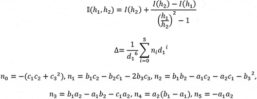
Notice that solvable quintics are defined by a reducible polynomial that can be factorized as a product of irreducible radicals. For the solvable quintics, we may define $d_1=y-n_4/5n_5$. This results the above Eqn. (76) into a reduced quintic

(77) $y^5+t{y}^3+u{y}^2+vy+w=0.$(77)

Hereby, the reduced parameters $\{t,u,v,w\}$ are described in Appendix C. The above reduced quintic as in Eqn. (77) is solvable if it is factorizable into lower degree polynomials with rational coefficients. Namely, it is factorized whenever the Cayley-resolvent (Farb & Wolfson, 2018) defined as

(78) ${\mathcal{C}}_r:=P^2-1024z{\stackrel{⌣}{\mathrm{\Delta }}}_0,$(78)

has a rational root in $z$. Here, the quintic discriminant ${\stackrel{⌣}{\mathrm{\Delta }}}_0$ and $P$ are defined in Appendix C. In particular, the above quintic is said to be solvable if the parameter

(79) $z=\frac{P^2}{1024{\stackrel{⌣}{\mathrm{\Delta }}}_0},$(79)

is a rational number. Hereby, a quintic is solved as a result of the Cayley-resolvent (Farb & Wolfson, 2018) that allows to test whether a given quintic is solvable or not.

Further, there exist implicit formulae such as Young/Lazard solutions for solving solvable quintics, see (Gray, 2018) for a historical introduction in the light of the abstract algebra. There are interesting solvable quintics such as Bring-Jerrard forms, Jacobi theta functions over a lattice index and number fields, elliptic modular forms, generalized hyper-geometric functions and their differential reductions, and computational aspects of a low genus curve (Bytev & Kniehl, 2016; Choie, Park, & Zagier, 2017; Skoruppa, 2015). In this regard, concerning solutions of quintic equations find their relations to algebraic geometry, viz. the rational curves, a pair of Calabi-Yau spaces, Abel-Jacobi maps, mirror symmetry, quintic $3$-folds and others (Candelas et al., 1991; Clemens, 1984; Cotterill, 2012; Cox & Katz, 1999; Johnsen & Kleiman, 1996).

As per this characterization, the behavior of the fluctuation discriminant $\mathrm{\Delta }$ is summarized in the next subsection.

5.3. Summary of the results

In this section, we summarize the results concerning stability properties of the Richardson numerical integration of an arbitrary real valued function as below.

5.3.1. Configurations with a constant numerator

From the observation of the cases (1, 2, 3, 4, 5, 6) having a single nonzero $n_i$, we find the following general expression of the discriminant

(80) $\mathrm{\Delta }=\frac{n_i}{{d_1}^{6-i}};i=0,1,2,3,4,5.$(80)

The behavior of the above constant numerators with a nonzero $n_i$ is tabulated in the Table 1.

Table 1. Stability of the configurations having a constant numerator with a nonzero $n_i$

	$i$ values for	The power $\mathit{i}$ of the denominator
$\mathit{i}$ values for vanishing ${\mathit{n}}_{\mathit{i}}$	nonzero ${\mathit{n}}_{\mathit{i}}$	${\mathit{d}}_{\mathbf{1}}^i$ of the discriminant $\mathrm{\Delta }$
5, 4, 3, 2, 1	0	6
5, 4, 3, 2, 0	1	5
5, 4, 3, 1, 0	2	4
5, 4, 2, 1, 0	3	3
5, 3, 2, 1, 0	4	2
4, 3, 2, 1, 0	5	1

5.3.2. Configurations with a linear numerator

For the above cases (7, 8, 9, 10, 11) with two nonzero $\{n_i,n_{i+1}\}$, it follows that we have

(81) $\mathrm{\Delta }=\frac{1}{d_1^{6-i}}(n_{i+1}{d}_1+n_i);i=0,1,2,3,4.$(81)

The classification of the stability of the Richardson integration of an integrable function corresponding to the above linear cases of $\mathrm{\Delta }$ as in Eqn. (81) arising with two nonzero $n_i$ is tabulated in Table 2 below

Table 2. Stability of the configurations having a linear numerator with two nonzero $n_i$

	$\mathit{i}$ values for	The power $\mathit{i}$ of the denominator
$\mathit{i}$ values for vanishing $n_i$	nonzero ${\mathit{n}}_{\mathit{i}}$	${\mathit{d}}_{\mathbf{1}}^i$ of the discriminant $\mathrm{\Delta }$
5, 4, 3, 2	1, 0	6
5, 4, 3, 0	2, 1	5
5, 4, 1, 0	3, 2	4
5, 2, 1, 0	4, 3	3
3, 2, 1, 0	5, 4	2

5.3.3. Configurations with a quadratic numerator

With the aforementioned observations as in the previous subsection, the quadratic cases of the numerator of $\mathrm{\Delta }$ can be divided into two categories. The first arises as the case of the three nonzero $\{n_i,n_{i+1},n_{i+2}\}$ or the three nonzero $\{n_i,n_{i+2},n_{i+4}\}$. The second arises as the case of the two nonzero$\{n_i,n_{i+2}\}$ or the two nonzero $\{n_i,n_{i+4}\}$. The respective values of the discriminant $\mathrm{\Delta }$ are given in Appendix D. In the sequel, we provide the tables corresponding to two different types of expressions of the discriminant. The stability properties of quadratic cases with three nonzero $n_i$ is tabulated in the Table 3 below.

Table 3. Stability of the configurations having a quadratic numerator with three nonzero $n_i$

	$\mathit{i}$ values for	The power $\mathit{i}$ of the denominator
$i$ values for vanishing ${\mathit{n}}_{\mathit{i}}$	nonzero ${\mathit{n}}_{\mathit{i}}$	${\mathit{d}}_{\mathbf{1}}^i$ of the discriminant $\mathrm{\Delta }$
5, 4, 3	2, 1, 0	6
5, 3, 1	4, 2, 0	6
5, 4, 0	3, 2, 1	5
4, 2, 0	5, 3, 1	5
5, 1, 0	4, 3, 2	4
2, 1, 0	5, 4, 3	3

The stability structures of the above quadratic cases with two nonzero $n_i$ is summarized in the below Table 4.

Table 4. Stability of the configurations having a quadratic numerator with two nonzero $n_i$

	$\mathit{i}$ values for	The power $\mathit{i}$ of the denominator
$i$ values for vanishing ${\mathit{n}}_{\mathit{i}}$	nonzero ${\mathit{n}}_{\mathit{i}}$	${\mathit{d}}_{\mathbf{1}}^i$ of the discriminant $\mathrm{\Delta }$
5, 4, 3, 1	2, 0	6
5, 3, 2, 1	4, 0	6
5, 4, 2, 0	3, 1	5
4, 3, 2, 0	5, 1	5
5, 3, 1, 0	4, 2	4
4, 2, 1, 0	5, 3	3

5.3.4. Configurations with a cubic numerator

As the cubic polynomial represented in Eqn. (71), there are four types of cubic discriminants that can be defined. They are the discriminants with four, three and two nonzero values of $n_i$. Their explicit expressions are referred in Appendix E. The stability properties of the cubic cases for different nonzero $n_i$ are tabulated in the below Table 5.

5.3.5. Configurations with a quartic numerator

The quartic numerator configurations can be categorized via their four types of nonzero discriminant as described in Appendix F. For various nonzero $n_i$, the stability structures of such quartic cases are summarized in the below Table 6.

Table 6. Stability of the configurations having a quartic numerator with different nonzero $n_i$

	$\mathit{i}$ values for	The power $\mathit{i}$ of the denominator
$i$ values for vanishing ${\mathit{n}}_{\mathit{i}}$	nonzero ${\mathit{n}}_{\mathit{i}}$	${\mathit{d}}_{\mathbf{1}}^i$ of the discriminant $\mathrm{\Delta }$
5	4, 3, 2, 1, 0	6
0	5, 4, 3, 2, 1	5
5, 1	4, 3, 2, 0	6
5, 2	4, 3, 1, 0	6
5, 3	4, 2, 1, 0	6
2, 0	5, 4, 3, 1	5
3, 0	5, 4, 2, 1	5
4, 0	5, 3, 2, 1	5
5, 2, 1	4, 3, 0	6
5, 3, 1	4, 2, 0	6
5, 3, 2	4, 1, 0	6
3, 2, 0	5, 4, 1	5
4, 2, 0	5, 3, 1	5
4, 3, 0	5, 2, 1	5
5, 3, 2, 1	4, 0	6
4, 3, 2, 0	5, 1	5

5.3.6. Configurations with a quintic numerator

The quintic numerator configurations can be divided into sixteen subcases of a nonzero discriminant. Their explicit values are given in Appendix G. The stability properties of the quintic cases for various nonzero $n_i$ are summarized in the Table 7 below.

Table 7. Stability of the configurations having a quintic numerator with different nonzero $n_i$

	$\mathit{i}$ values for	The power $\mathit{i}$ of the denominator
$i$ values for vanishing ${\mathit{n}}_{\mathit{i}}$	nonzero ${\mathit{n}}_{\mathit{i}}$	${\mathit{d}}_{\mathbf{1}}^i$ of the discriminant $\mathrm{\Delta }$
0	5, 4, 3, 2, 1, 0	6
1	5, 4, 3, 2, 0	6
2	5, 4, 3, 1, 0	6
3	5, 4, 2, 1, 0	6
4	5, 3, 2, 1, 0	6
2, 1	5, 4, 3, 0	6
3, 1	5, 4, 2, 0	6
4, 1	5, 3, 2, 0	6
3, 2	5, 4, 1, 0	6
4, 2	5, 3, 1, 0	6
4, 3	5, 2, 1, 0	6
3, 2, 1	5, 4, 0	6
4, 2, 1	5, 3, 0	6
4, 3, 1	5, 2, 0	6
4, 3, 2	5, 1, 0	6
4, 3, 2, 1	5, 0	6

6. Future scope of the work

In this section, having provided the optimization analysis of the Richardson numerical integration for an arbitrary real valued function, we discuss its perspective applications under variations of its step sizes. Namely, we examine the behavior of flow components as the first derivative and fluctuation capacities as the pure second derivatives of the Richardson numerical integration for an arbitrary real valued function. The critical points of the Richardson integration scheme arise as the roots of its flow equations. Hereby, for a given real valued smooth function, we have shown that its critical points are expressible as a function of roots of the flow components. At a given pair of step sizes, this yields a pair of quadrature equations in the step size parameters $d_1$. As a function of the step sizes, these equations are simultaneously solved in order to get critical points of the Richardson integration of a given real valued function.

Hitherto, from the perspective of reliability theories, we have obtained all possible critical points of the Richardson numerical integration of an arbitrary smooth real valued function. Furthermore, in the space of step sizes, we have shown that the origin is a repeated root of the flow equations. Namely, it is shown that the origin arises as a nontrivial repeated root along with four other simple roots as the critical points of the Richardson integration of a real valued function, see Eqn. (32). In order to discuss the stability of an arbitrary Richardson integration, we have computed the concerned fluctuation capacities as its pure second order partial derivatives.

In the sequel, we have calculated the undermining local correlation between the step sizes as its mixed second order partial derivative. At a given critical point, we have offered the global stability of the Richardson numerical integration via the sign of the fluctuation discriminant. It is explicitly demonstrated that the numerator of the fluctuation discriminant arises as a fifth order polynomial in the aforementioned step size parameter $d_1$ of the Richardson integration.

6.1. Sensitivity analysis

Optimization of the Richardson numerical integration of an arbitrary real valued smooth function finds applications in various domains of science and engineering. For example, in the light of the optimization theory and Richardson extrapolation models, a sensitivity analysis can be performed for analog circuits with a multi-objective function. Namely, by considering an evolutionary approach, a multi-parameter sensitivity analysis exists in a number of recent studies. Such investigations find their relevance in estimating the partial derivatives that govern the sensitivities of performances of a given amplifier. Thereby, one can compare the variations of sizes of the metal-oxide-semiconductor field-effect-transistors (MOSFET), see (Guerra-Gómez, Tlelo-Cuautle, & Luis, 2013) for an overview of the Richardson extrapolation analysis, multi-stage optimization and their applications to analog circuits.

6.2. Finite difference schemes

Applications of the Richardson extrapolation model are in practice as finite difference schemes towards the solution of ordinary and partial differential equations with an increased accuracy. The success of a finite linear Richardson model depends on the existence a rapidly converging asymptotic expansion over errors of the solution (Blum, Lin, & Rannacher, 1986) as a finite linear sum. Hereby, as an asymptotic error expansion, the Richardson extrapolation models offer a numerical understanding of a system of difference equations as a combination of finite linear elements. In this regard, the Ref. (Roos, Stynes, & Tobiska, 2008) offers robust numerical solutions for certain singularly perturbed differential equations and that of the Ref. (Křížek & Pekka, 1987) provides the associated super-convergence techniques.

6.3. Non-uniform grids solutions

As an application towards non-uniform grid solutions, the Richardson extrapolation model can be used to examine the grid independence of the solutions with a given grid refinement parameter. A solution with variable grid refinement factors in the coordinate directions is anticipated to offer the optimal numerical solution with the right degree of the convergence (Celik & Karatekin, 1997). The associated safety factors are discussed in (Xing & Stern, 2010) in the light of the fluid mechanics. There exists a number of engineering optimizations with non-uniform grid solutions. This includes the optimal shape design, dimensional reduction, geometric variability assessment, meta-models and deterministic particle swarm, see (Chen et al., 2015) towards global robust architecture techniques and high-fidelity optimizations.

6.4. Numerical weather forecasting

The fluid mechanical global optimization methods offer applications of our model towards the test of the system reliability (Chen et al., 2015; Xing & Stern, 2010) and robust design techniques for ships operability in an uncertain ocean environment in real time (Diez, Chen, Campana, & Stern, 2013). Hereby, our model supports the optimal numerical weather prediction (Bauer, Thorpe, & Brunet, 2015; Mason, 1986) in the light of the Richardson’s original dream as the atmospheric circulation and forecasting of the weather as a time integration.

6.5. Discrete dynamical systems

Our analysis is well-suited towards the intrinsic stability examination of discrete dynamical systems such as a heuristic search planning over certain hybrid domains (Ramirez, Scala, Haslum, & Thiebaux, 2017), stochastic modeling in business industry (Zhi-Sheng & Xie, 2015) and their role in finance engineering (Lamberton & Lapeyre, 2011), charge carrier transport and ion vacancy dynamics, solar technology and their mathematical modeling (Courtier, Richardson, & Foster, 2018). Further studies exist towards the Runge-Kutta type numerical integration techniques (Kalogiratou, Monovasilis, Psihoyios, & Simos, 2014). This comprises of a system of ordinary or partial differential equations and their stability analysis as well as the error adjustment, case control analysis and applications in environmental sciences, e.g., Canadian INTEROCC study (Oraby et al., 2018).

7 Summary and conclusion

In this paper, we have focused on optimization of the Richardson numerical integration of an arbitrary real valued integrable function under the variations of its step sizes. Considering the fact that there always exists an error in a numerical integral of an arbitrary real valued function, we have investigated the nature of its optimization and convergence properties in the space of step sizes. In the sequel, we have shown that our method optimizes the value of a definite Richardson integral than its conventional evaluations. Specifically, in the space of step sizes, we have examined the nature of stabilities of the Richardson integral of an arbitrary real valued function about its critical points. Mathematically, our analysis shows that the optimal value of the Richardson integral arises directly via its extremization over step sizes. In general, we find that such an optimization holds for any smooth real valued function. To be precise, our investigation offers a stable Richardson numerical integration scheme with the optimal value of errors. This results in an intrinsic classification of the Richardson integration of arbitrary integrable functions in the space of step sizes.

Richardson method is among the most efficient numerical integrations that is analyzed under variations of its multiple step sizes $\{h_1,h_2\}$. We have examined the optimization of the Richardson model that contains the trapezium rule and Romberg integration as its special cases. With the fact that the Richardson integration depends on a pair of step sizes, we have investigated its stability as a two variable function. Our analysis optimizes the Richardson integration of an arbitrary real valued function under fluctuations of its step sizes. Hereby, the critical points of the Richardson integration are defined as a pair of flow equations in the step sizes. For an arbitrary real valued smooth function, the critical points arise as roots of the flow equations. In particular, the flow equations that arise as a function of the step sizes need to be simultaneously solved in order to get the critical points of the Richardson integration. In general, this yields a pair of nonlinear equations in $h_1$ and $h_2$.

To be specific, given two distinct step sizes $\{h_1,h_2\}$, we have obtained all possible critical points of the Richardson integration of an arbitrary integrable function. Consequently, the fluctuation capacities as the auto-correlations between the step sizes are computed as the pure second order derivatives of the Richardson integration. At a given critical point, the global stability of the Richardson numerical integration is governed by the sign of the fluctuation discriminant. Hereby, we find that the discriminant arises as a fifth order polynomial in the step size parameter $d_1$, viz. the square of the ratio of the step sizes around the unity. Following the above estimation, we have discussed the nature of critical points of the Richardson numerical integration and classified its stability domains in various limiting cases of the discriminant. In order to make our analysis comprehensible, we have provided a flowchart and tabular descriptions of the results toward an intrinsic classification of the stability structures of the Richardson integration of arbitrary real valued functions. Subsequently, under variations of the step sizes $\{h_1,h_2\}$, a detailed discussion of the stability properties of the Richardson numerical integration is provided in the cases when the numerator of its fluctuation discriminant arises as an equation of the degree less than or equal to five in the factor $d_1$. In the light of optimization theory, associated algebraic perspectives are considered under the agenda of the present research investigation, as well.

As a special case of the Richardson integration, we have discussed the optimization of the Romberg integration of an arbitrary real valued function as a weighted extrapolation model. As mentioned before, the notion of the Romberg integration arises as a special case of the present consideration. Herewith, by optimizing the Richardson integration, we have optimized the Simpson $1/3$ or $3/8$ values of a numerical integral, or the trapezium rule as a suitable convex combination of given intervals of the integration. It is worth emphasizing that the optimization of the Richardson integration equally optimizes various limiting numerical integrations, as well. Moreover, we have given qualitative analysis of the Richardson integration and its optimization with its relevance to existing theoretical and experimental models. As a future scope of this research, we have highlighted perspectives from the sensitivity analysis, finite difference schemes, non-uniform grids, forecasting of the weather as a time integration and the original Richardson’s dream toward the atmospheric circulation as well as discrete dynamical systems.

In the light of numerical practices, the significance of the results is that our analysis gives polynomial type stability criteria for the Richardson integration of an arbitrary integrable function under variations of its step sizes. In this discussion, a comparative analysis of the proposed optimization technique with the other existing quadrature methods and practical practices are left open for a future study. On the other hand, we considered the number of steps $(b-a)/h_j$ while performing the Richardson integration in the light of the randomized algorithms of Agrawal and Biswas. Hereby, it follows that both step sizes $h_1$ and $h_2$ are randomized and they give a correct partition of the integration interval $(a,b)$ in the derandomization limit. Investigations of such processes to obtain a correctly derandomized optimization task with integer valued steps as the optimization constraints are among the future research scope.

Finally, it is worth mentioning that our analysis can be applied to both the classical numerical algorithms that are solutions of a given system of differential equations, and to other advanced numerical methods in the realm of different permutations, combinations and splitting procedures, e.g., label switching, multi-modality and population structures (Jakobsson & Rosenberg, 2007). From the perspective of the present analysis, classical numerical algorithms are devised and supplemented either as the corresponding supervised, semi-supervised or unsupervised solutions (Huang, Song, Gupta, & Cheng, 2014). Hereby, the following two issues are important: (a) a large time-step and two small time-steps need to be handled by using the same numerical method, and (b) the order of the selected numerical integration should be given prior to an initiation of the algorithm, see (Bousquet & Elisseeff, 2002) towards the machine learning and stable Richardson techniques. Industrial applications of the proposed study are the subject matter of future research and developments.

Cover image

Source: Author.

Acknowledgements

The first author would like to thank the Yukawa Institute for Theoretical Physics at Kyoto University. Discussions during the workshop YITP-T-18-04 “New Frontiers in String Theory 2018” were useful to complete this work.

Additional information

Funding

The authors received no direct funding for this research.

Notes on contributors

Bhupendra Nath Tiwari

Dr. Bhupendra Nath Tiwari an alumnus of Jawaharlal Nehru University New Delhi, and Indian Institute of Technology Kanpur, India is an Assistant Professor at the University of Information Science and Technology, “St. Paul the Apostle”, Ohrid, Macedonia; act as Ricercatore, Visiting Scientist, PDF at INFN-Laboratori Nazionali di Frascati, Rome, Italy. He has published research papers, reviews, books and monographs (in English & French). Having qualified UGC-FRP, CSIR-JRF/NET/SRF, GATE, GRE, TOEFL and CILS, he is a professional body member of the AMS, IOP, APS, MDPI, IEEE, Springer, Elsevier, World Scientific Publications and Hindawi Publishing Corporation, Worldwide. His research interests include theoretical and mathematical aspects of S&T. Er. Amarasingha Arachchige Mihiri Chathurika is a master candidate at the University of Information Science and Technology, “St. Paul the Apostle”, Ohrid, Macedonia. She is Machine Learning trainee at Lightblue Technology, Tokyo, Japan who aspires to work as a Machine Learning Engineer.

Appendix

In the squeal, we provide explicit expression for coefficient of solutions of the cubic, quartic and quintic equations and their associated with the stability quantities as in section 5. In each of the above cases, we have given explicit values of the fluctuation discriminant in order to classify the nature of the local and global stabilities of the configurations with their discriminants as a cubic, quartic and quintic polynomials in the step size parameter $d_1$. Further, we give the associated limiting values of the discriminants corresponding to the quadratic, cubic, quartic and quintic configurations for different values of the coefficients $n_i$.

Appendix A.

In this Appendix, we provide the quantities associated with the cubic discriminant as a limiting configuration undermining the Richardson numerical integration of an arbitrary real valued function under fluctuations of the step sizes $(h_1,h_2)$. Given the cubic polynomial as in Eqn. (71), following (Nickalls, 1993), the parameters $\{{\mathrm{\Delta }}_0,{\mathrm{\Delta }}_1,C_1,\omega \}$ and discriminant ${\mathrm{\Delta }}_2$ characterizing its solutions $\{d_1^{(k)}|k=1,2,3\}$ are given by

(82) ${\mathrm{\Delta }}_0={{\tilde{n}}_2}^2-3{\tilde{n}}_3{\tilde{n}}_1,$(82)

(83) ${\mathrm{\Delta }}_1=2{{\tilde{n}}_2}^3-9{\tilde{n}}_3{\tilde{n}}_2{\tilde{n}}_1+27{{\tilde{n}}_3}^2{\tilde{n}}_0,$(83)

(84) $C_1=\sqrt[3]{\frac{{\mathrm{\Delta }}_1\pm \sqrt{{{\mathrm{\Delta }}_1}^2-4{{\mathrm{\Delta }}_0}^3}}{2}},$(84)

(85) $\omega =\frac{-1+\sqrt{3}i}{2}.$(85)

Here, the coefficients $\{n_i|i=0,1,2,3,4,5\}$ governing the above cubic roots read as in Eqn. (34). We see (Nickalls, 1993) that the discriminant ${\mathrm{\Delta }}_2$ classifying the nature of roots of the cubic equation as in Eqn. (71) is given by

(86) $\begin{array}{cc}{\mathrm{\Delta }}_2=& 18{\tilde{n}}_3{\tilde{n}}_2{\tilde{n}}_1{\tilde{n}}_0-4{{\tilde{n}}_2}^3{\tilde{n}}_0+{{\tilde{n}}_2}^2{{\tilde{n}}_1}^2-4{\tilde{n}}_3{{\tilde{n}}_1}^3-27{{\tilde{n}}_3}^2{{\tilde{n}}_0}^2.\end{array}$(86)

Following the above description, the associated stability results concerning the Richardson numerical integration of an arbitrary real valued function are summarized in the Table 5.

Appendix B.

In this Appendix, we give the quantities associated with the quartic discriminant as a limiting configuration undermining the Richardson integration of an arbitrary real valued function under fluctuations of its step sizes $(h_1,h_2)$. In particular, given the quartic polynomial as in Eqn. (73), the solutions $\{d_1^{(i)}|i=1,2,3,4\}$ as in Eqns. (74, 75) of the corresponding quartic equation are obtained (Lazard, 1988; Rees, 1922) in terms of the following parameters

(87) $S=\frac{1}{2}\sqrt{-\frac{2}{3}p+\frac{1}{3{\stackrel{⌣}{n}}_4}\left(Q+\frac{{\tilde{\mathrm{\Delta }}}_0}{Q}\right)},$(87)

(88) $Q=\sqrt[3]{\frac{{\tilde{\mathrm{\Delta }}}_1+\sqrt{{{\tilde{\mathrm{\Delta }}}_1}^2-4{{\tilde{\mathrm{\Delta }}}_0}^3}}{2}},$(88)

Here, the terms $p,r,{\tilde{\mathrm{\Delta }}}_0,{\tilde{\mathrm{\Delta }}}_1$ are defined according as

(89) $p=\frac{8{\stackrel{⌣}{n}}_4{\stackrel{⌣}{n}}_2-3{{\stackrel{⌣}{n}}_3}^2}{8{{\stackrel{⌣}{n}}_4}^2},$(89)

(90) $r=\frac{{{\stackrel{⌣}{n}}_3}^3-4{\stackrel{⌣}{n}}_4{\stackrel{⌣}{n}}_3{\stackrel{⌣}{n}}_2+8{{\stackrel{⌣}{n}}_4}^2{\stackrel{⌣}{n}}_1}{8{{\stackrel{⌣}{n}}_4}^3},$(90)

(91) ${\tilde{\mathrm{\Delta }}}_0={{\stackrel{⌣}{n}}_2}^2-3{\stackrel{⌣}{n}}_3{\stackrel{⌣}{n}}_1+12{\stackrel{⌣}{n}}_4{\stackrel{⌣}{n}}_0,$(91)

(92) $\begin{array}{cc}{\tilde{\mathrm{\Delta }}}_1=& 2{{\stackrel{⌣}{n}}_2}^3-9{\stackrel{⌣}{n}}_3{\stackrel{⌣}{n}}_2{\stackrel{⌣}{n}}_1+27{{\stackrel{⌣}{n}}_3}^2{\stackrel{⌣}{n}}_0+27{\stackrel{⌣}{n}}_4{{\stackrel{⌣}{n}}_1}^2-72{\stackrel{⌣}{n}}_4{\stackrel{⌣}{n}}_2{\stackrel{⌣}{n}}_0.\end{array}$(92)

The classification of the roots $\{d_1^{(i)}|i=1,2,3,4\}$ of the quartic equation is determined (Lazard, 1988; Rees, 1922) by the sign of the discriminant

(93) $\begin{array}{rl}{\tilde{\mathrm{\Delta }}}_2=& 256{{\stackrel{⌣}{n}}_4}^3{{\stackrel{⌣}{n}}_0}^3-192{{\stackrel{⌣}{n}}_4}^2{\stackrel{⌣}{n}}_3{\stackrel{⌣}{n}}_1{{\stackrel{⌣}{n}}_0}^2-128{{\stackrel{⌣}{n}}_4}^2{{\stackrel{⌣}{n}}_2}^2{{\stackrel{⌣}{n}}_0}^2+144{{\stackrel{⌣}{n}}_4}^2{\stackrel{⌣}{n}}_2{{\stackrel{⌣}{n}}_1}^2{\stackrel{⌣}{n}}_0\\ & -27{{\stackrel{⌣}{n}}_4}^2{{\stackrel{⌣}{n}}_1}^4+144{\stackrel{⌣}{n}}_4{{\stackrel{⌣}{n}}_3}^2{\stackrel{⌣}{n}}_2{{\stackrel{⌣}{n}}_0}^2-6{\stackrel{⌣}{n}}_4{{\stackrel{⌣}{n}}_3}^2{{\stackrel{⌣}{n}}_1}^2{\stackrel{⌣}{n}}_0-80{\stackrel{⌣}{n}}_4{\stackrel{⌣}{n}}_3{{\stackrel{⌣}{n}}_2}^2{\stackrel{⌣}{n}}_1{\stackrel{⌣}{n}}_0\\ & +18{\stackrel{⌣}{n}}_4{\stackrel{⌣}{n}}_3{\stackrel{⌣}{n}}_2{{\stackrel{⌣}{n}}_1}^3+16{\stackrel{⌣}{n}}_4{{\stackrel{⌣}{n}}_2}^4{\stackrel{⌣}{n}}_0-4{\stackrel{⌣}{n}}_4{{\stackrel{⌣}{n}}_2}^3{{\stackrel{⌣}{n}}_1}^2-27{{\stackrel{⌣}{n}}_3}^4{{\stackrel{⌣}{n}}_0}^2+18{{\stackrel{⌣}{n}}_3}^3{\stackrel{⌣}{n}}_2{\stackrel{⌣}{n}}_1{\stackrel{⌣}{n}}_0\\ & -4{{\stackrel{⌣}{n}}_3}^3{{\stackrel{⌣}{n}}_1}^3-4{{\stackrel{⌣}{n}}_3}^2{{\stackrel{⌣}{n}}_2}^3{\stackrel{⌣}{n}}_0+{{\stackrel{⌣}{n}}_3}^2{{\stackrel{⌣}{n}}_2}^2{{\stackrel{⌣}{n}}_1}^2,\end{array}$(93)

and that of the parameters $P,R,$ and $D$ defined as

(94) $P=8{\stackrel{⌣}{n}}_4{\stackrel{⌣}{n}}_2-3{{\stackrel{⌣}{n}}_3}^2,$(94)

(95) $R={{\stackrel{⌣}{n}}_3}^3+8{{\stackrel{⌣}{n}}_4}^2{\stackrel{⌣}{n}}_1-4{\stackrel{⌣}{n}}_4{\stackrel{⌣}{n}}_3{\stackrel{⌣}{n}}_2,$(95)

(96) $\begin{array}{cc}D=& 64{{\stackrel{⌣}{n}}_4}^3{\stackrel{⌣}{n}}_0-16{{\stackrel{⌣}{n}}_4}^2{{\stackrel{⌣}{n}}_2}^2+16{\stackrel{⌣}{n}}_4{{\stackrel{⌣}{n}}_3}^2{\stackrel{⌣}{n}}_2-16{{\stackrel{⌣}{n}}_4}^2{\stackrel{⌣}{n}}_3{\stackrel{⌣}{n}}_1-3{{\stackrel{⌣}{n}}_3}^4.\end{array}$(96)

Appendix C.

In this Appendix, we provide the coefficient of a quintic equation as in Eqn. (77) and the associated Cayley criterion to check whether a given quintic is solvable or not (Farb & Wolfson, 2018). Namely, for a given configuration with its discriminant as a quintic equation in $d_1$ as in Eqn. (76), we can check its solvability by defining a reduced quintic as in Eqn. (77). Hereby, it follows (Farb & Wolfson, 2018; Gray, 2018) that the coefficients $\{t,u,v,w\}$ of the reduced quintic are given by

(97) $\begin{array}{rl}& t=\frac{5n_5{n}_3-2{n_2}^2}{5{n_5}^2},\\ & u=\frac{25{n_5}^2{n}_2-15n_5{n}_4{n}_3+4{n_4}^3}{25{n_5}^3},\\ & v=\frac{125{n_5}^3{n}_1-50{n_5}^2{n}_4{n}_2+15n_5{n_4}^2{n}_3-3{n_4}^4}{125{n_5}^4},\\ & w=\frac{1}{3125{n_5}^5}(3125{n_5}^4{n}_0-625{n_5}^3{n}_4{n}_1+125{n_5}^2{n_4}^2{n}_2-25n_5{n_4}^3{n}_3+4{n_4}^5).\end{array}$(97)

The nature of the roots of a quintic equation [71, 72] as in Eqn. (76) is described by the factorizability of the Cayley-resolvent ${\mathcal{C}}_r$ as in Eqn. (78), where the parameters $\{P,{\stackrel{⌣}{\mathrm{\Delta }}}_0\}$ read according as

(98) $\begin{array}{rl}& P=z^3-z^2(20v+3t^2)-z(8t^{2}v-16t{u}^2-240v^2+400wu-3t^4)-t^6+28t^{4}v\\ & -16t^3{u}^2-176t^2{v}^2-80t^{2}uw+224t{u}^{2}v-64u^4+4000t{w}^2+320v^3-1600uvw,\end{array}$(98)

(99) $\begin{array}{rl}{\stackrel{⌣}{\mathrm{\Delta }}}_0=& -128t^2{v}^4+3125w^4-72t^{4}uvw+560t^{2}u{v}^{2}w+16t^4{v}^3+256v^5+108t^5{w}^2\\ \hspace{0.17em}& -1600u{v}^{3}w+144t{u}^2{v}^3-900t^3{v}^{2}w+2000t{v}^2{w}^2-3750tu{w}^3+825t^2{u}^{2}w\\ \hspace{0.17em}& +2250u^{2}v{w}^2+108u^{5}w-27u^4{v}^2-630t{u}^{3}vw+16t^3{u}^{3}w-4t^3{u}^2{v}^2.\end{array}$(99)

Appendix D.

In this Appendix, following the section 5.3.3, we give explicit values of the limiting discriminant $\mathrm{\Delta }$ when its numerator correspond to a quadratic or a reducible quadratic equation in $d_1$. For the quadratic cases of the numerator of $\mathrm{\Delta }$ with three nonzero coefficients $\{n_i,n_{i+1},n_{i+2}\}$ as in section 5.3.3, it is direct to see that $\mathrm{\Delta }$ is given by

(100) $\mathrm{\Delta }=\frac{1}{d_1^{6-i}}(n_{i+2}{d}_1^2+n_{i+1}{d}_1+n_i);i=0,1,2,3.$(100)

Similarly, for three nonzero coefficients $\{n_i,n_{i+2},n_{i+4}\}$, we find that the discriminant $\mathrm{\Delta }$ reads as

(101) $\mathrm{\Delta }=\frac{1}{d_1^{6-i}}(n_{i+4}{d}_1^4+n_{i+2}{d}_1^2+n_i);i=0,1.$(101)

On the other hand, for two nonzero coefficients $\{n_i,n_{i+2}\}$, the discriminant $\mathrm{\Delta }$ simplifies as

(102) $\mathrm{\Delta }=\frac{1}{{d_1}^{6-i}}(n_{i+2}{d}_1^2+n_i);i=0,1,2,3.$(102)

Finally, for two nonzero coefficients $\{n_i,n_{i+4}\}$, we observe the following discriminant

(103) $\mathrm{\Delta }=\frac{1}{d_1^{6-i}}(n_{i+4}{d}_1^4+n_i);i=0,1.$(103)

Appendix E.

In this Appendix, we give explicit values of the fluctuation discriminant $\mathrm{\Delta }$ when its numerator arises as a cubic polynomial in $d_1$ as in Eqn. (71). The associated expressions of the discriminant $\mathrm{\Delta }$ with four, three and two nonzero values of the coefficients $n_i$ are summarized as below

(104) $\mathrm{\Delta }=\frac{1}{d_1^{6-i}}(n_{i+3}{d}_1^3+n_{i+2}{d}_1^2+n_{i+1}{d}_1+n_i);i=0,1,2,$(104)

(105) $\mathrm{\Delta }=\frac{1}{d_1^{6-i}}(n_{i+3}{d}_1^3+n_{i+2}{d}_1^2+n_i);i=0,1,2,$(105)

(106) $\mathrm{\Delta }=\frac{1}{d_1^{6-i}}(n_{i+3}{d}_1^3+n_{i+1}{d}_1+n_i);i=0,1,2,$(106)

(107) $\mathrm{\Delta }=\frac{1}{d_1^{6-i}}(n_{i+3}{d}_1^3+n_i);i=0,1,2.$(107)

Appendix F.

In this Appendix, we offer the respective expressions of the discriminant $\mathrm{\Delta }$ when its numerator corresponds to a quartic polynomial in the step size parameter $d_1$ as in Eqn. (73). In this case, it follows that $\mathrm{\Delta }$ with its quartic numerator having either five, four, three or two nonzero coefficients $n_i$ are described as per the following expressions

(108) $\mathrm{\Delta }=\frac{1}{d_1^{6-i}}(n_{i+4}{d}_1^4+n_{i+3}{d}_1^3+n_{i+2}{d}_1^2+n_{i+1}{d}_1+n_i);i=0,1,$(108)

(109) $\mathrm{\Delta }=\frac{1}{d_1^{6-i}}(n_{i+4}{d}_1^4+n_{i+3}{d}_1^3+n_{i+2}{d}_1^2+n_i);i=0,1,$(109)

(110) $\mathrm{\Delta }=\frac{1}{d_1^{6-i}}(n_{i+4}{d}_1^4+n_{i+3}{d}_1^3+n_{i+1}{d}_1+n_i);i=0,1,$(110)

(111) $\mathrm{\Delta }=\frac{1}{d_1^{6-i}}(n_{i+4}{d}_1^4+n_{i+2}{d}_1^2+n_{i+1}{d}_1+n_i);i=0,1,$(111)

(112) $\mathrm{\Delta }=\frac{1}{d_1^{6-i}}(n_{i+4}{d}_1^4+n_{i+3}{d}_1^3+n_i);i=0,1,$(112)

(113) $\mathrm{\Delta }=\frac{1}{d_1^{6-i}}(n_{i+4}{d}_1^4+n_{i+2}{d}_1^2+n_i);i=0,1,$(113)

(114) $\mathrm{\Delta }=\frac{1}{d_1^{6-i}}(n_{i+4}{d}_1^4+n_{i+1}{d}_1+n_i);i=0,1,$(114)

(115) $\mathrm{\Delta }=\frac{1}{d_1^{6-i}}(n_{i+4}{d}_1^4+n_i);i=0,1.$(115)

Appendix G.

Finally, in this Appendix, we provide the expressions of the fluctuation discriminant $\mathrm{\Delta }$ as discussed in section 5.3.6. In this case, the numerator of the discriminant $\mathrm{\Delta }$ corresponds to a class of quintic polynomials with different set of nonzero $n_i$. The explicit expressions of $\mathrm{\Delta }$ are given as follow

(116) $\mathrm{\Delta }=\frac{1}{d_1^6}(n_5{d}_1^5+n_4{d}_1^4+n_3{d}_1^3+n_2{d}_1^2+n_1{d}_1+n_0),$(116)

(117) $\mathrm{\Delta }=\frac{1}{d_1^6}(n_5{d}_1^5+n_4{d}_1^4+n_3{d}_1^3+n_2{d}_1^2+n_0),$(117)

(118) $\mathrm{\Delta }=\frac{1}{d_1^6}(n_5{d}_1^5+n_4{d}_1^4+n_3{d}_1^3+n_1{d}_1+n_0),$(118)

(119) $\mathrm{\Delta }=\frac{1}{d_1^6}(n_5{d}_1^5+n_4{d}_1^4+n_2{d}_1^2+n_1{d}_1+n_0),$(119)

(120) $\mathrm{\Delta }=\frac{1}{d_1^6}(n_5{d}_1^5+n_3{d}_1^3+n_2{d}_1^2+n_1{d}_1+n_0),$(120)

(121) $\mathrm{\Delta }=\frac{1}{d_1^6}(n_5{d}_1^5+n_4{d}_1^4+n_3{d}_1^3+n_0),$(121)

(122) $\mathrm{\Delta }=\frac{1}{d_1^6}(n_5{d}_1^5+n_4{d}_1^4+n_2{d}_1^2+n_0),$(122)

(123) $\mathrm{\Delta }=\frac{1}{d_1^6}(n_5{d}_1^5+n_3{d}_1^4+n_1{d}_1+n_0),$(123)

(124) $\mathrm{\Delta }=\frac{1}{d_1^6}(n_5{d}_1^5+n_3{d}_1^3+n_2{d}_1^2+n_0),$(124)

(125) $\mathrm{\Delta }=\frac{1}{d_1^6}(n_5{d}_1^5+n_3{d}_1^3+n_1{d}_1+n_0),$(125)

(126) $\mathrm{\Delta }=\frac{1}{d_1^6}(n_5{d}_1^5+n_2{d}_1^2+n_1{d}_1+n_0),$(126)

(127) $\mathrm{\Delta }=\frac{1}{d_1^6}(n_5{d}_1^5+n_4{d}_1^4+n_0),$(127)

(128) $\mathrm{\Delta }=\frac{1}{d_1^6}(n_5{d}_1^5+n_3{d}_1^3+n_0),$(128)

(129) $\mathrm{\Delta }=\frac{1}{d_1^6}(n_5{d}_1^5+n_2{d}_1^2+n_0),$(129)

(130) $\mathrm{\Delta }=\frac{1}{d_1^6}(n_5{d}_1^5+n_1{d}_1+n_0),$(130)

(131) $\mathrm{\Delta }=\frac{1}{d_1^6}(n_5{d}_1^5+n_0).$(131)

References

- Agrawal, M., & Biswas, S. (2003). Primality and identity testing via Chinese remaindeing. Journal of the ACM (JACM), 50(4), 429–36.
- Alekseev, V. B. (2004). Abels theorem in problems and solutions: Based on the lectures of professor VI Arnold. Netherlands: Springer Science & Business Media. doi:10.1007/1-4020-2187-9
- Angelis, C. D. (1994). Self-trapped propagation in the nonlinear cubic-quintic Schrodinger equation: A variational approach. IEEE Journal of Quantum Electronics, 30(3), 818–821. doi:10.1109/3.286174
- Artin, E. (2007). Algebra with Galois theory (Vol. 15). American Mathematical Soc. Courant Lecture Notes. Providence, US. ISBN: 978-0-8218-4129-7
- Asmussen, S., & Albrecher, H. (2010). Ruin probabilities. World Scientific Publishing Co Pte Ltd, Singapore, ISBN13: 9789814282529.
- Bao-Quan, A., Wang, X.-J., Liu, G.-T., Wen, D.-H., Xie, H.-Z., Chen, W., & Liu, L. G. (2003). Efficiency optimization in a correlation ratchet with asymmetric unbiased fluctuations. Physical Review E, 68(6), 061105. doi:10.1103/PhysRevE.68.061105
- Battaglia, M., Berge, J., Case, S., Yoobin, J., Ryoo, J., & Wichrowski, N. (2015). AMSC460/CMSC460: Computational methods group project 4: Extrapolation in numerical integration. AMSC460 / CMSC460 Computational Methods, Spring 2015, University of Maryland, Maryland, USA.
- Bauer, F. L., Rutishauser, H., & Stiefel, E. (1963). New aspects in numerical quadrature. Proceedings of Symposia in Applied Mathematics, 15, 199–218.
- Bauer, P., Thorpe, A., & Brunet, G. (2015). The quiet revolution of numerical weather prediction. Nature, 525(7567), 47. doi:10.1038/525S9a
- Bellucci, S., Tiwari, B. N., & Gupta, N. (2012). Geometrical methods for power network analysis. Berlin, Heidelberg: Springer Science & Business Media. doi:10.1007/978-3-642-33344-6.
- Blum, H., Lin, Q., & Rannacher, R. (1986). Asymptotic error expansion and Richardson extranpolation for linear finite elements. Numerische Mathematik, 49(1), 11–37. doi:10.1007/BF01389427
- Bousquet, O., & Elisseeff, A. (2002, mar). Stability and generalization. J. Mach. Learn. Res., 2, 499–526.
- Bytev, V. V., & Kniehl, B. A. (2016). HYPERDIRE - HYPERgeometric functions dIfferential rEduction: Mathematica-based packages for the differential reduction of generalized hypergeometric functions: Lauricella function FC of three variables. Computer Physics Communications, 206, 78–83. doi:10.1016/j.cpc.2016.04.016
- Cabrera, S. D., & Parks, T. W. (1991). Extrapolation and spectral estimation with iterative weighted norm modification. IEEE Transactions on Signal Processing, 39(4), 842–851. doi:10.1109/78.80906
- Candelas, P., Xenia, C., Green, P. S., & Parkes, L. (1991). A pair of Calabi-Yau manifolds as an exactly soluble superconformal theory. Nuclear Physics B, 359(1), 21–74. doi:10.1016/0550-3213(91)90292-6
- Castan˜eda, P. P. (2002). Second-order homogenization estimates for nonlinear composites incorporating field fluctuations: Itheory. Journal of the Mechanics and Physics of Solids, 50(4), 737–757. doi:10.1016/S0022-5096(01)00099-0
- Celik, I., & Karatekin, O. (1997). Numerical experiments on application of Richardson extrapolation with nonuniform grids. Journal of Fluids Engineering, 119(3), 584–590.
- Changpin, L., & Zeng, F. (2015). Numerical methods for fractional calculus. Boca Raton: Chapman and Hal- l/CRC, Taylor & Francis.
- Chapra, S. C., & Canale, R. P. (1998). Numerical methods for engineers (Vol. 2). New York: Mcgraw- hill.
- Chen, X., Diez, M., Kandasamy, M., Zhang, Z., Campana, E. F., & Stern, F. (2015). High-fidelity global optimization of shape design by dimensionality reduction, metamodels and deterministic particle swarm. Engineering Optimization, 47(4), 473–494. doi:10.1080/0305215X.2014.895340
- Choie, Y., Park, Y. K., & Zagier, D. (2017). Periods of modular forms on Γ 0(N)and products of Jacobi theta functions (arXiv preprint arXiv:1706.07885).
- Ciarlet, P. G. (2001). Handbook of numerical analysis (Vol. 8, pp. 650). Amsterdam: Elsevier. ISBN: 9780444509062.
- Clarkson, P. A. (1993). Applications of analytic and geometric methods to nonlinear differential equations (Vol. 413). Netherlands: Springer Science & Business Media. doi:10.1007/978-94-011-2082-1
- Clemens, H. (1984). Some results about Abel-Jacobi mappings. Topics in Transcendental Algebraic Geometry, 106, 289–304.
- Cöster, K., & Schmidt, K. P. (2016). Extracting critical exponents for sequences of numerical data via series extrapolation techniques. Physical Review E, 94(2), 022101. doi:10.1103/PhysRevE.94.022101
- Cotterill, E. (2012). Rational curves of degree 11 on a general quintic 3-fold. Quarterly Journal of Mathematics, 63(3), 539–568. doi:10.1093/qmath/har001
- Courtier, N. E., Richardson, G., & Foster, J. M. (2018). A fast and robust numerical scheme for solving models of charge carrier transport and ion vacancy motion in perovskite solar cells. Applied Mathematical Modelling, 63, 329–348. doi:10.1016/j.apm.2018.06.051
- Cox, D. A., & Katz, S. (1999). Mirror symmetry and algebraic geometry (Vol. 68). Providence, RI: American Mathematical Society.
- Deb, K. (2005) Multi-Objective Optimization. In Burke E.K., & Kendall G. (Eds.), Search Methodologies. Springer, Boston, MA, USA. Online ISBN: 978-0-387-28356-2. doi: 10.1007/0-387-28356-0_10.
- Diez, M., Chen, X., Campana, E. F., & Stern, F. (2013). Reliability-based robust design optimization for ships in real ocean environment. In 12th International Conference on Fast Sea Transportation, FAST2013, Amsterdam, The Netherlands.
- Dimov, I., Zlatev, Z., & Faragó. (2017). Richardson extrapolation: Practical aspects and applications (Vol. 2). Berlin: Walter de Gruyter GmbH & Co KG (ASIN: B06Y65J6ZT).
- Faragó, I., Havasi, Á., & Zlatev, Z. (2010). Efficient implementation of stable Richardson extrapolation algorithms. Computers & Mathematics with Applications, 60(8), 2309–2325. doi:10.1016/j.camwa.2010.08.025
- Farb, B., & Wolfson, J. (2018). Resolvent degree, Hilbert’s 13th problem and geometry (arXiv preprint arXiv:1803.04063)
- Feller, W. (2015). Fluctuation Theory Of Recurrent Events. In: Schilling R., Vondraček Z., & Woyczyński W. (eds), Selected Papers I. Springer, Cham, Online ISBN: 978-3-319-16859-3.doi:10.1007/978-3-319-16859-3_43
- Gao, G.-H., Sun, Z.-Z., & Zhang, H.-W. (2014). A new fractional numerical differentiation formula to approximate the Caputo fractional derivative and its applications. Journal of Computational Physics, 259, 33–50. doi:10.1016/j.jcp.2013.11.017
- Gray, J. (2018). Revision and first assignment. Chapter in The Book-- a History of Abstract Algebra, from Algebraic Equations to Modern Algebra. Springer International Publishing (Ebook). ISBN: 978-3-319-94773-0. doi: 10.1007/978-3-319-94773-0
- Guerra-Gómez, I., Tlelo-Cuautle, E., & Luis, G. (2013). Richardson extrapolation-based sensitivity analysis in the multi-objective optimization of analog circuits. Applied Mathematics and Computation, 222, 167–176. doi:10.1016/j.amc.2013.07.059
- Gupta, N., Tiwari, B. N., & Bellucci, S. (2013). Intrinsic geometric analysis of the network reliability and voltage stability. International Journal of Electrical Power & Energy Systems, 44(1), 872–879. doi:10.1016/j.ijepes.2012.08.032
- Hairer, E., Lubich, C., & Wanner, G. (2006). Geometric numerical integration: Structure-preserving algorithms for ordinary differential equations (Vol. 31). Berlin Heidelberg: Springer Science & Business Media. doi:10.1007/3-540-30666-8
- Harkey, J. A., & Kenny, T. W. (2000). 1/f noise considerations for the design and process optimization of piezoresistive cantilevers. Journal of Microelectromechanical Systems, 9(2), 226–235. doi:10.1109/84.846703
- Huang, G., Song, S., Gupta, J. N. D., & Cheng, W. (2014). Semi-supervised and unsupervised extreme learning machines. IEEE Transactions on Cybernetics, 44(12), 2405–2417. doi:10.1109/TCYB.2014.2307349
- Hundsdorfer, W., & Verwer, J. G. (2013). Numerical solution of time-dependent advection-diffusion- reaction equations (Vol. 33). Berlin Heidelberg: Springer Science & Business Media. doi:10.1007/978-3-662-09017-6
- Igoe, W. B. (1967). Application of Richardson’s extrapolation to numerical evaluation of sonic-boom integrals. Washington, DC: NASA Technical Note D 3806.
- Jakobsson, M., & Rosenberg, N. A. (2007). CLUMPP: A cluster matching and permutation program for dealing with label switching and multimodality in analysis of population structure. Bioinformatics, 23(14), 1801–1806. doi:10.1093/bioinformatics/btm233
- Johnsen, T., & Kleiman, S. L. (1996). Rational curves of degree at most 9 on a general quintic threefold. Communications in Algebra, 24(8), 2721–2753. doi:10.1080/00927879608542652
- Kalogiratou, Z., Monovasilis, T., Psihoyios, G. Y., & Simos, T. E. (2014). Runge–Kutta type methods with special properties for the numerical integration of ordinary differential equations. Physics Reports, 536(3), 75–146. doi:10.1016/j.physrep.2013.11.003
- Kappe, L.-C., & Warren, B. (1989). An elementary test for the Galois group of a quartic polynomial. The American Mathematical Monthly, 96(2), 133–137. doi:10.1080/00029890.1989.11972158
- Kaw, A., & Krivanek, J. (2018). Measuring errors, 01.02, Holistic numerical methods, transforming numerical education for the STEM undergraduate. The University of South Florida, Florida, USA
- Keller, H. B. (2018). Numerical methods for two-point boundary-value problems. New York, NY: Courier Dover Publications.
- Khargonekar, P. P., Petersen, I. R., & Zhou, K. (1990). Robust stabilization of uncertain linear systems: Quadratic stabilizability and H/sup infinity/control theory. IEEE Transactions on Automatic Control, 35(3), 356–361. doi:10.1109/9.50357
- Kincaid, D., Kincaid, D. R., & Cheney, E. W. (2009). Numerical analysis: Mathematics of scientific computing (Vol. 2). Providence, RI: American Mathematical Soc.
- Kiusalaas, J. (2013). Numerical methods in engineering with Python 3. Cambridge: Cambridge university press.
- Kozioł, A., & Wiśniewski, R. (2008). Optimization of the quintic equation of the state based model for the calculations of different thermodynamic properties. Polish Journal of Chemical Technology, 10(1), 6–10. doi:10.2478/v10026-008-0002-x
- Křížek, M., & Pekka, N. (1987). On superconvergence techniques. Acta Applicandae Mathematica, 9(3), 175–198. doi:10.1007/BF00047538
- Křížek, M., & Somer, L. (2015). Why quintic polynomial equations are not solvable in radicals. Application of Mathematics, 2015, 125–131.
- Kuipo, J. K., Tiwari, B. N., Gupta, N., Khosravy, M., Bellucci, S., & Marina, N. (2016). An introduction to dynamic optical optimization. Universal Journal of Engineering Science, 4(3), 45-49, SAN JOSE, CA: Horizon Research Publishing. doi:10.13189/ujes.2016.040302
- Kushner, H. J. (1967). Stochastic stability and control (Technical report). BROWN UNIV PROVIDENCE RI.
- Lambers, J. V., & Sumner, A. C. (2016). Explorations in numerical analysis. Irvine, CA: University of California at Irvine.
- Lambert, J. D. (1991). Numerical methods for ordinary differential systems: The initial value problem. New York, NY: John Wiley & Sons, Inc.. ISBN:0-471-92990-5
- Lamberton, D., & Lapeyre, B. (2011). Introduction to stochastic calculus applied to finance. Boca Raton, Florida: Chapman and Hall/CRC, Taylor & Francis.
- Lazard, D. (1988). Quantifier elimination: Optimal solution for two classical examples. Journal of Symbolic Computation, 5(1–2), 261–266. doi:10.1016/S0747-7171(88)80015-4
- Lei, X., Chengjun, W., & Chen, P. (2018). Optimizing parameter of particle damping based on Leidenfrost effect of particle flows. Mechanical Systems and Signal Processing, 104, 60–71. doi:10.1016/j.ymssp.2017.10.037
- Little, R. J. A., & Rubin, D. B. (2014). Statistical analysis with missing data (Vol. 333). Hoboken, NJ: John Wiley & Sons.
- Liu, E. H. (2006). Fundamental methods of numerical extrapolation with applications. Mitopencourse- Ware, Massachusetts Institute of Technology, 209(2), 022101.
- Maharani, M., Salhi, A., & Suharto, R. A. (2018). Enhancing the stability of Lanczos- type algorithms by embedding interpolation and extrapolation for the solution of systems of linear equations. Journal of Mathematical and Fundamental Sciences, 50(2), 148–165. doi:10.5614/j.math.fund.sci.2018.50.2.4
- Marino, R. (1997). Adaptive control of nonlinear systems: Basic results and applications. Annual Reviews in Control, 21, 55–66. doi:10.1016/S1367-5788(97)00033-3
- Mason, B. J. (1986). Numerical weather prediction. Proceedings of the Royal Society A: Mathematical, Physical and Engineering Sciences, 407(1832), 51–60. doi:10.1098/rspa.1986.0083
- Mona, T., Lagzi, I., & Havasi, Á. (2015). Solving reaction-diffusion and advection problems with Richardson extrapolation (pp. 9). Journal of Chemistry, 2015. doi:10.1155/2015/350362
- Nickalls, R. W. D. (1993). A new approach to solving the cubic: Cardans solution revealed. The Mathematical Gazette, 77(480), 354–359. doi:10.2307/3619777
- Oraby, T., Sivaganesan, S., Bowman, J. D., Kincl, L., Richardson, L., McBride, M., … Krewski, D. (2018). Berkson error adjustment and other exposure surrogates in occupational case-control studies, with application to the Canadian INTEROCC study. Journal of Exposure Science and Environmental Epidemiology, 28(3), 251. doi:10.1038/jes.2017.2
- Ott, E. (2002). Chaos in dynamical systems. Cambridge, UK: Cambridge university press. Online ISBN: 9780511803260. doi:10.1017/CBO9780511803260
- Ouannas, A., & Odibat, Z. (2015). Generalized synchronization of different dimensional chaotic dynamical systems in discrete time. Nonlinear Dynamics, 81(1–2), 765–771. doi:10.1007/s11071-015-2026-0
- Parikh, N., & Boyd, S. (2014). Proximal algorithms. Foundations and Trends in Optimization, 1(3), 127–239. doi:10.1561/2400000003
- Podlubny, I. (1998). Fractional differential equations: An introduction to fractional derivatives, fractional differential equations, to methods of their solution and some of their applications (Vol. 198). Cambridge, Massachusetts: Elsevier.
- Ramirez, M., Scala, E., Haslum, P., & Thiebaux, S. (2017). Numerical integration and dynamic discretization in heuristic search planning over hybrid domains (arXiv preprint arXiv:1703.04232)
- Rees, E. L. (1922). Graphical discussion of the roots of a quartic equation. The American Mathematical Monthly, 29(2), 51–55. doi:10.1080/00029890.1922.11986100
- Roos, H.-G., Stynes, M., & Tobiska, L. (2008). Robust numerical methods for singularly perturbed differential equations: Convection-diffusion-reaction and flow problems (Vol. 24). Washington, DC: Taylor & Francis for the Mathematical Association of America.
- Ruffini, P. (1799). Teoria generale delle equazioni: In cui si dimostra impossibile la soluzione algebraica delle equazioni generali di grad superiore al quarto (Vol. 1). Nella stamperia di ST d’Aquino. Michigan, USA: University of Michigan.
- Ruppeiner, G. (1995). Riemannian geometry in thermodynamic fluctuation theory. Reviews of Modern Physics, 67(3), 605. doi:10.1103/RevModPhys.67.605
- Ruyer-Quil, C., & Manneville, P. (2002). Further accuracy and convergence results on the modeling of flows down inclined planes by weighted-residual approximations. Physics of Fluids, 14(1), 170–183. doi:10.1063/1.1426103
- Saitou, K., Izui, K., Nishiwaki, S., & Papalambros, P. (2005). A survey of structural optimization in mechanical product development. Journal of Computing and Information Science in Engineering, 5(3), 214–226. doi:10.1115/1.2013290
- Samoradnitsky, G. (2017). Stable non-Gaussian random processes: Stochastic models with infinite variance. Abingdon, UK: Routledge.
- Schmidt, J. W., & Henrici, P. (1966). Discrete variable methods in ordinary differential equations. XI+ 407 S. m. Abb. u. Tab. New York/London 1962. John Wiley & Sons. ZAMM-Journal of Applied Mathematics and Mechanics/Zeitschrift Für Angewandte Mathematik Und Mechanik, 46(5), 327–328. doi:10.1002/zamm.19660460521
- Skoruppa, N. (2015). Explicit methods in the theory of Jacobi forms of lattice index and over number fields. ICERM Modular Forms and Curves of Low Genus: Computational Aspects.Providence, RI:ICERM Programs.
- Stoer, J., & Bulirsch, R. (2013). Introduction to numerical analysis (Vol. 12). New York, NY: Springer Science & Business Media.
- Tiwari, B. N. (2008). Sur les corrections de la géométrie thermodynamique des trous noirs. Editions universitaires europeennes ISBN-13: 978-6131535390, arXiv preprint arXiv:0801.4087.
- Tiwari, B. N. (2011a). Geometric perspective of entropy function: Embedding, spectrum and convexity. Saarbrucken, Germany: LAP LAMBERT Academic Publishing. ISBN-13, 978–3845431789.
- Tiwari, B. N. (2011b, September 26). On generalized uncertainty principle (arXiv preprint arXiv:0801.3402). LAP LAMBERT Academic Publishing, ISBN-13: 978-3846515327.
- Tiwari, B. N., Kuipo, J. K., Bellucci, S., & Marina, N. (2016). On extensions of the optical optimization. American Scientific Research Journal for Engineering, Technology, and Sciences (ASRJETS), 26(1), 302–313.
- Wen, C.-K., Wang, C.-J., Jin, S., Wong, K.-K., & Ting, P. (2016, May). Bayes-optimal joint channel-and-data estimation for massive MIMO with low-precision ADCs. IEEE Transactions on Signal Processing, 64(10), 2541–2556. doi:10.1109/TSP.2015.2508786
- Xie, X.-F., Zhang, W.-J., & Yang, Z.-L. (2002). Dissipative particle swarm optimization. In Evolutionary computation, 2002. CEC’02. proceedings of the 2002 congress, Computer Society, Washington, DC (vol. 2, 1456–1461). IEEE.
- Xing, T., & Stern, F. (2010). Factors of safety for Richardson extrapolation. Journal of Fluids Engineering, 132(6), 061403. doi:10.1115/1.4001771
- Zhi-Sheng, Y., & Xie, M. (2015). Stochastic modelling and analysis of degradation for highly reliable products. Applied Stochastic Models in Business and Industry, 31(1), 16–32. doi:10.1002/asmb.2063
- Zimmermann, H.-J. (1975). Description and optimization of fuzzy systems. International Journal of General System, 2(1), 209–215. doi:10.1080/03081077508960870