Local asymptotic normality and efficient estimation for multivariate GINAR(p) models

Abstract

We derive the Local Asymptotic Normality (LAN) property for a multivariate generalized integer-valued autoregressive (MGINAR) process with order p. The generalized thinning operator in the MGINAR(p) process includes not only the usual Binomial thinning but also Poisson thinning, geometric thinning, Negative Binomial thinning and so on. By using the LAN property, we propose an efficient estimation method for the parameter of the MGINAR(p) process. Our procedure is based on the one-step method, which update initial $\sqrt{n}$-consistent estimators to efficient ones. The one-step method has advantages in both computational simplicity and efficiency. Some numerical results for the asymptotic relative efficiency (ARE) of our estimators and the CLS estimators are presented. In addition, a real data analysis is provided to illustrate the application of the proposed estimation method.

Keywords:

• integer-valued time series
• thinning operations
• LAN
• efficient estimation

PUBLIC INTEREST STATEMENT

We derive the Local Asymptotic Normality (LAN) property for a multivariate generalized integer-valued autoregressive (MGINAR) process with order p. recently, there has been a growing interest in modelling discrete-valued time series that arise in various fields of statistics.

The MGINAR process is one of the class of discrete-valued time series models and contains various classes. By using the LAN property, we propose an efficient estimation method for the parameter. Our procedure is based on the one-step method, which update initial root-n consistent estimators to efficient ones. The one-step method has advantages in both computational simplicity and efficiency. Some numerical results for the asymptotic relative efficiency (ARE) of our estimators and the CLS estimators are presented. In addition, a real data analysis is provided to illustrate the application of the proposed estimation method.

1. Introduction

Recently, there has been a growing interest in modelling discrete-valued time series that arise in various fields of statistics (e.g., Weiß, 2018). This paper is concerned with a special class of observation-driven models termed “integer-valued autoregressive processes” (INAR processes), which were introduced independently by Al-Osh and Alzaid (1987) and McKenzie (1985, 1988). They introduced the integer-valued autoregressive process with order 1 (INAR(1) process) to model non-negative integer-valued phenomena with time dependence. The more general INAR(p) processes were considered by Alzaid and Al-Osh (1990), Du and Li (1991) and so on. The INAR process consists of a mixture both of the distribution of thinning operator and the distribution of the innovation process. Alzaid and Al-Osh (1990) discussed the INAR(p) process in case that the thinning operator follows Binomial distribution (i.e., specified), while the distribution of the innovation process is left unspecified. Latour (1998) introduced a generalized version of the INAR(p) process, namely, the causal and stationary generalized integer-valued autoregressive (GINAR(p)) process. The generalized thinning operator in the GINAR(p) process includes not only the usual Binomial thinning but also Poisson thinning, Geometric thinning, and Negative Binomial thinning (by Ristić, Bakouch, & Nastić, 2009). The above history is appropriate for the univariate case. Nowadays, extensions for the multivariate case are being actively researched and applied. One of the first approaches to multivariate thinning mechanism was by McKenzie (1988). After that, Franke and Subba Rao (1993) introduced a multivariate INAR(1) (MINAR(1)) model based on independent Binomial thinning operators. The extensions for the MINAR(1) model were discussed by Latour (1997), Karlis and Pedeli (2013), and so on. This paper discusses a parameter estimation problem for a multivariate version of the GINAR(p) (MGINAR($p$)) process. The MGINAR model is quite a large class, including all the models described above.

Estimation of the parameter for the INAR($p$) process can be carried out in a variety of ways. Common ways for estimating parameters include the method of moments (MM), based on the Yule-Walker equations, and conditional least squares (CLS). The main advantage of both approaches is their simplicity due to the closed-form formulae and robustness due to require no assumption for the distribution. It is known that MM and CLS estimators are asymptotically equivalent. However, Al-Osh and Alzaid (1987) and so on have recommended using maximum likelihood (ML) estimators instead of MM and CLS estimators because they are less biased for small sample sizes. However, it is well known that the ML method is computationally unattractive due to complicated transition probabilities, including many convolutions. To overcome this problem, Drost, Van Den Akker, and Werker (2008) considered one-step, asymptotically efficient estimation of the INAR($p$) model. Their method can reduce high computational cost due to the convolutions involved in the ML method. Following Drost et al. (2008), this paper provides a one-step method, which update initial $\sqrt{n}-$consistent estimators to efficient ones for the MGINAR ($p$) processes. In the class of multivariate integer-valued models, the number of convolutions involved in the likelihood function is very large. For some distributions with reproductive property, the likelihood can be simplified, but it is impossible to apply such a simplification for all models in the MGINAR ($p$) processes. Therefore, it would be quite important to reduce the computational cost by using a one-step estimation. We first establish the local asymptotic normality (LAN) structure for experiments of the MGINAR ($p$) process. Considering the CLS estimator as the initial estimator, a one-step update estimator is proposed. We can also show that this estimator is asymptotically efficient.

The organization of this paper is as follows. In Section 2, the MGINAR ($p$) process is introduced and the LAN property is established. Section 3 discusses the efficient estimation. The CLS estimator is introduced and its asymptotic property is shown. Then, by using the LAN property, a one-step estimator is proposed to update the CLS estimator. In Section 4, the asymptotic relative efficiency (ARE) of the one-step estimator and the CLS estimator is examined through some simulation experiments. In addition, a real data analysis is provided to illustrate the application of the proposed estimation method. The proofs and other details are included in the Appendix.

2. The LAN property

Let $\{{\mathit{X}}_t=(X_{1,t},\dots ,X_{d,t}{)}^T;t\in {\mathbb{Z}}_{+}=\mathbb{N}\cup \{0\}\}$ be a $d$- dimensional non-negative integer-valued random process (i.e., ${\mathit{X}}_t(\omega )\in {\mathbb{Z}}_{+}^d$). The multivariate generalized integer-valued autoregressive process of order $p$ (MGINAR($p$)) is defined by

(1) ${\mathit{X}}_t=\sum _{k=1}^p{A}^{(k)}\circ {\mathit{X}}_{t-k}+{ϵ}_t$(1)

where ${\mathit{A}}^{(k)}=(A_{i,j}^{(k)}{)}_{t,j=1,\dots ,d}$ is a $d\times d$-matrix for $k=1,\dots ,p$ and the matrix thinning ${\mathit{A}}^{(k)}\circ {\mathit{X}}_{t-k}$ gives a $d$-dimensional random vector with $i$th component

(2) ${\left[{\mathit{A}}^{(k)}\circ {\mathit{X}}_{t-k}\right]}_i=\sum _{j=1}^d{A}_{i,j}^{(k)}\circ X_{j,t-k}=\sum _{j=1}^d\sum _{r=1}^{X_{j,t-k}}{\xi }_{i,j,r}^{(k)},i=1,\dots ,d.$(2)

Note that for any $A\in \mathbb{R}$, $A\circ 0=0$; $\{{\xi }_{i,j,r}^{(k)};r\in {\mathbb{Z}}_{+}\}$ is a collection of independent and identically distributed (i.i.d.), non-negative, integer-valued random variables with the distribution function $G_{A_{i,j}^{(k)}}$ and the mean $A_{i,j}^{(k)}$; $\left\{{ϵ}_t={({ϵ}_{1,t},\dots ,{ϵ}_{d,t})}^{\mathrm{T}};t\in {\mathbb{Z}}_{+}\right\}$ is a collection of i.i.d. non-negative, integer-valued random vectors, where the $i$th component ${ϵ}_{i,t}$ has an independent distribution function $F_{a_i}$ and the mean $a_i$. Suppose that the starting values $\{{\mathit{X}}_{-p},\dots ,{\mathit{X}}_{-1}\}$ have a distribution $\nu$ on ${\mathbb{Z}}_{+}^{d\times p}$, and $\left\{{\mathit{X}}_{-p},\dots ,{\mathit{X}}_{-1}\right\},\left\{{\xi }_{i,j,r}^{(1)}\right\},\dots ,\left\{{\xi }_{i,j,r}^{(p)}\right\},\left\{ϵ\right\}$.

are independent of each other.

Throughout the paper, the number of lags ($p\in \mathbb{N}$) and the dimensions ($d\in \mathbb{N}$) are fixed and known. Let $F$ and $G$ denote the classes of distributions of $ϵ$ and $\xi$ that belong to parametric classes, respectively, say $F\equiv (F_a;a\in {\mathrm{\Theta }}_a)$ and $G\equiv (G_A;A\in {\mathrm{\Theta }}_A)$. For instance, when we consider the Binomial thinning operator and the Binomial innovation, $F$ and $G$ should be defined by $F_a(x)=a^x(1-a{)}^x$ and $G_A(x)=A^x(1-A{)}^x$ for $a\in {\mathrm{\Theta }}_a=(0,1),A\in {\mathrm{\Theta }}_A=(0,1)$, and $x\in \{0,1\}$. Our goal is to estimate the parameter $\theta =(a^{\mathrm{T}},A^{\mathrm{T}}{)}^{\mathrm{T}}\in \mathrm{\Theta }\subset {\mathbb{R}}^q$ with $q=d+d^{2}p$, efficiently, where

$\mathrm{\Theta }=\left\{{(a^{\mathrm{T}},\mathit{A}{}^{\mathrm{T}})}^{\mathrm{T}};\mathit{a}=(a_1,\dots ,a_d{)}^{\mathrm{T}}\in {\mathrm{\Theta }}_a^d,\mathit{A}=\mathrm{v}\mathrm{e}\mathrm{c}{(\mathit{A}{}^{(1)},\dots ,\mathit{A}{}^{(p)})}^{\mathrm{T}}=(A_{1,1}^{(1)},\dots ,A_{d,d}^{(p)}{)}^{\mathrm{T}}\in {\mathrm{\Theta }}_A^{d^{2}p}\right\}.$

For (probability) measures $F_1,\dots ,F_k\in F\cup G$, we introduce the following notations for the convolutions:

• $F_1$_⊛$F_2$: the convolution of $F_1$ and $F_2$

• _⊛${ }_{k=1,\dots ,p}{F}_k$: the convolution of $F_1,\dots ,F_k$ (i.e., _⊛${ }_{k=1,\dots ,p}{F}_k=F_1$_⊛$\cdots$_⊛$F_k$)

• $F_1^{n⊛}$ : the $n$ times convolution of $F_1$ (i.e., $F_1^{n⊛}=\stackrel{ntimes}{\overbrace{F_1⊛\dots ⊛F_1}}$)

Based on the above notations, we consider the corresponding probability space for $\{{\mathit{X}}_t\}$ denoted by $(\mathrm{\Omega },\mathcal{F},{\mathbb{P}}_{\nu ,\theta ,F,G})$, where $\mathrm{\Omega }$ is a sample space, $\mathcal{F}$ is the $\sigma$-algebra, and ${\mathbb{P}}_{\nu ,\theta ,F,G}$ is the probability measure given by $\nu$ (distribution of $\{{\mathit{X}}_{-p},\dots ,{\mathit{X}}_{-1}\}$), $\theta$ (parameter), $F$ (class of distribution of $ϵ$) and $G$ (class of distribution of $\xi$). Furthermore, we introduce $\mathbb{F}=\{{\mathcal{F}}_t;t\ge -p\}$ as the natural filtration generated by $\{{\mathit{X}}_{-p},\dots ,{\mathit{X}}_t\}$ (i.e. ${\mathcal{F}}_t=\sigma ({\mathit{X}}_{-p},\dots ,{\mathit{X}}_t)\ne \sigma ({\mathit{X}}_{-p},\dots ,{\mathit{X}}_{-1},ϵ{}_0,\dots ,ϵ{}_t)$).

From (1) and (2), we can write

${\mathit{X}}_t=\sum _{k=1}^p\sum _{j=1}^d\sum _{r=1}^{X_{j,t-k}}{\xi }_{j,r}^{(k)}+ϵ{}_t$

where ${\xi }_{j,r}^{(k)}=({\xi }_{1,j,r}^{(k)},\dots ,{\xi }_{d,j,r}^{(k)}{)}^{\mathrm{T}}$. Hence, it follows, for any $t\in {\mathbb{Z}}_{+}$,

$\begin{array}{rl}& {\mathbb{P}}_{\nu ,\theta ,F,G}\{{\mathit{X}}_t=x_t|{\mathcal{F}}_{t-1}\}={\mathbb{P}}_{\nu ,\theta ,F,G}\{{\mathit{X}}_t=x_t|{\mathit{X}}_{t-1},\dots ,{\mathit{X}}_{t-p}\}\\ & :=P_{(X_{t-1},\dots ,X_{t-p}),x_t}^{\theta }(\mathrm{s}\mathrm{a}\mathrm{y})\end{array}$

For some $x_{t-k}=(x_{1,t-k},\dots ,x_{d,t-k}{)}^{\mathrm{T}}\in {\mathbb{Z}}_{+}^d,k=0,1,\dots ,p$, the transition probability $P_{(x_{t-1},\dots ,x_{t-p}),x_t}^{\theta }$ is given by

$P_{(x_{t-1},\dots ,x_{t-p}),x_t}^{\theta }={\mathbb{P}}_{\nu ,\theta ,F,G}\left\{{\mathit{X}}_t=x_t|{\mathit{X}}_{t-1}=x_{t-1},\dots ,{\mathit{X}}_{t-p}=x_{t-p}\right\}={\mathbb{P}}_{\nu ,\theta ,F,G}\left\{\sum _{k=1}^p\sum _{j=1}^d\sum _{r=1}^{X_{j,t-k}}{\xi }_{j,r}^{(k)}+{ϵ}_t=x_t|{\mathit{X}}_{t-1}=x_{t-1},\dots ,{\mathit{X}}_{t-p}=x_{t-p}\right\}=\prod _{i=1}^d{\mathbb{P}}_{\nu ,\theta ,F,G}\left\{\sum _{k=1}^p\sum _{j=1}^d\sum _{r=1}^{X_{j,t-k}}{\xi }_{i,j,r}^{(k)}+{ϵ}_{i,t}=x_{i,t}|{\mathit{X}}_{t-1}=x_{t-1},\dots ,{\mathit{X}}_{t-p}=x_{t-p}\right\}=\prod _{i=1}^d\left\{F_{a_i⊛}\left({ }_{\begin{array}{c}⊛k=1,\dots ,p\\ j=1,\dots ,d\end{array}}{G}_{A_{i,j}^{(k)}}^{x_{j,t-k⊛}}\right)\right\}(x_{i,t}).$

We consider parametric MGINAR models in which the parameter space is restricted to the stationary parameter space, for instance, in case of the Binomial thinning operator and $d=1$, the thinning part of the parameter space should be defined by $\{A;A=(A^{(1)},\dots ,A^{(p)}{)}^{\mathrm{T}}\in (0,1{)}^d,{\sum }_{k=1}^p{A}^{(k)}<1\}$. Suppose that $\mathcal{F}\times \mathcal{G}$ is a combination of a family of parametric distributions for the thinning operator and innovation (immigrant) with the formula below:

$\mathcal{F}=\{F_a=(F_{a_1},\dots ,F_{a_d});a=(a_1,\dots ,a_d{)}^{\mathrm{T}}\in {\mathbb{R}}^d\}$

$\mathcal{G}=\{G_A=(G_{A_{1,1}^{(1)}},\dots ,G_{A_{d,d}^{(p)}});\mathit{A}=\mathrm{v}\mathrm{e}\mathrm{c}({\mathit{A}}^{(1)},\dots ,{\mathit{A}}^{(p)}{)}^{\mathrm{T}}=(A_{1,1}^{(1)},\dots ,A_{d,d}^{(p)}{)}^{\mathrm{T}}\in {\mathbb{R}}^{d^{2}p}\}$

Suppose that for any $\mathit{\theta }=(a^{\mathrm{T}},{\mathit{A}}^{\mathrm{T}}{)}^{\mathrm{T}}\in \mathrm{\Theta }$, $\{{\mathit{X}}_t\}$ with $F_{\mathbf{a}}\times G_{\mathbf{A}}\in \mathcal{F}\times \mathcal{G}$ is a strictly stationary process. Let ${\mathbb{P}}_{\nu ,\theta ,F,G}^{(n)}$ denote the law of $\{{\mathit{X}}_{-p},\dots ,{\mathit{X}}_n\}$ on the measurable space $\left({\mathbb{Z}}_{+}^{d(n+1+p)},{\mathbb{N}}^{{\mathbb{Z}}_{+}^{d(n+1+p)}}\right)$ under ${\mathbb{P}}_{\nu ,\theta ,F,G}$. Here ${\mathbb{Z}}_{+}^{d(n+1+p)}$ is the sample space and the power set ${\mathbb{N}}^{{\mathbb{Z}}_{+}^{d(n+1+p)}}$ is the $\sigma$-algebra on this sample space. Observing $({\mathit{X}}_{-p},\dots ,{\mathit{X}}_n)$ yields the following sequence of experiments:

${\mathcal{E}}^{(n)}(\nu ,\mathrm{\Theta },F,G)=\left({\mathbb{Z}}_{+}^{d(n+1+p)},{\mathbb{N}}^{{\mathbb{Z}}_{+}^{d(n+1+p)}},\left({\mathbb{P}}_{\nu ,\theta ,F,G}^{(n)};\theta \in \mathrm{\Theta }\right)\right),n\in {\mathbb{Z}}_{+}$

where the initial distribution $\nu$ is fixed and the distributions for the thinning operator and innovation (immigrant) are parametrized (i.e., once $\theta =(a^{\mathrm{T}},\mathit{A}{}^{\mathrm{T}}{)}^{\mathrm{T}}\in \mathrm{\Theta }$ is fixed, the distributions are given by $F_{\mathbf{a}}$ and $G_{\mathbf{A}}$).

To prove the LAN property for the sequence of experiments ${\mathcal{E}}^{(n)}(\nu ,\mathrm{\Theta },F,G),n\in {\mathbb{Z}}_{+}$, we impose the following assumptions.

Assumption 1 . (A1) $\mathrm{\Theta }$ is an open, convex subset of ${\mathbb{R}}^q$ with $q=d+d^{2}p$.

(A2) The supports of $F_a$ and $G_A$ do not depend on $\mathit{a}$ and $\mathit{A}$ and we have, for all $\theta =(a^{\mathrm{T}},{\mathit{A}}^{\mathrm{T}}{)}^{\mathrm{T}},F_a(0)\times G_A(0)\in (0,1{)}^{d\times d^{2}p}$.

(A3) For all $e\in {\mathbb{Z}}_{+}$ and all $\theta =(a{}^{\mathrm{T}},{\mathit{A}}^{\mathrm{T}}{)}^{\mathrm{T}}=((a_i),(A_{i,j}^{(k)}){)}^{\mathrm{T}}\in \mathrm{\Theta }$,

$f_{a_i}(e)=\frac{\mathrm{\partial }{F}_{a_i}}{\mathrm{\partial }{a}_i}(e),{\dot{f}}_{a_i}(e)=\frac{{\mathrm{\partial }}^2{F}_{a_i}}{{(\mathrm{\partial }{a}_i)}^2}(e),g_{A_{i,j}^{(k)}}(e)=\frac{\mathrm{\partial }{G}_{A_{i,j}^{(k)}}}{\mathrm{\partial }{A}_{i,j}^{(k)}}(e),{\dot{g}}_{A_{i,j}^{(k)}}(e)=\frac{{\mathrm{\partial }}^2{G}_{A_{i,j}^{(k)}}}{{(\mathrm{\partial }{A}_{i,j}^{(k)})}^2}(e)$

are defined, continuous in $\mathrm{\Theta }$, and satisfied with $\frac{\mathrm{\partial }{F}_{a_{i^{\prime }}}}{\mathrm{\partial }{a}_i}=0,\frac{\mathrm{\partial }{G}_{A_{i^{\prime },j^{\prime }}^{(k^{\prime })}}}{\mathrm{\partial }{A}_{i,j}^{(k)}}=0$ for $i\ne i^{\prime },(i,j,k)\ne (i^{\prime },j^{\prime },k^{\prime })$, respectively.

(A4) Let $sup(\cdot )$ denotes

$sup(Z):=\mathrm{s}\mathrm{u}{\mathrm{p}}_{\tilde{\theta }=(({\tilde{a}}_i),({\tilde{A}}_{i,j}^{(k)}{))}^{\mathrm{T}};\parallel \tilde{\theta }-\theta \parallel <\delta }{\mathbb{E}}_{\nu ,\tilde{\theta },F,G}\left[Z|\mathit{X}{}_{-p},\dots ,\mathit{X}{}_0\right].$

For every $\theta \in \mathrm{\Theta }$, there exist a $\delta >0$ and a random variable $M^{\theta }$ such that for all $i,j=1,\dots ,d,k=1,\dots ,p$, $sup(|f_{{\tilde{a}}_i}({ϵ}_{i,0}){|}^2)\le M^{\theta }$, $sup(|{\dot{f}}_{{\tilde{a}}_i}({ϵ}_{i,0})|)\le M^{\theta }$, $sup(|g_{{\tilde{A}}_{i,j}^{(k)}}({\xi }_{i,j,1}){|}^2)\le M^{\theta }$, $sup(|{\dot{g}}_{{\tilde{A}}_{i,j}^{(k)}}({\xi }_{i,j,1})|)\le M^{\theta }$, and ${\mathbb{E}}_{\nu ,\theta ,F,G}[M^{\theta }]<\mathrm{\infty }$.

(A5) Let ${\dot{\mathrm{\ell }}}_n$ and ${\ddot{\mathrm{\ell }}}_n$ be the first and second derivatives of log-likelihood for $\{X_{-p},\dots ,X_n\}$. The information equality ${\mathbb{E}}_{\nu ,\theta ,F,G}[{\dot{\mathrm{\ell }}}_n{\dot{\mathrm{\ell }}}_n^{\mathrm{T}}]=-{\mathbb{E}}_{\nu ,\theta ,F,G}[{\ddot{\mathrm{\ell }}}_n]$ is satisfied, and ${\mathbb{E}}_{\nu ,\theta ,F,G}[{\dot{\mathrm{\ell }}}_n{\dot{\mathrm{\ell }}}_n^{\mathrm{T}}]$ is nonsingular and continuous in $\mathrm{\Theta }$.

(A6) For all $\theta \in \mathrm{\Theta }$, $\parallel {\mathbb{E}}_{\nu ,\theta ,F,G}[{ϵ}_0{ϵ}_0^{\mathrm{T}}]\parallel <\mathrm{\infty }$ and $\parallel {\mathbb{E}}_{\nu ,\theta ,F,G}[{\mathit{X}}_0{\mathit{X}}_0^{\mathrm{T}}]\parallel <\mathrm{\infty }$.

(A7) $F_a\times G_A=F_{a^{\prime }}\times G_{A^{\prime }}$ implies $(a,\mathit{A})=(a^{\prime },{\mathit{A}}^{\prime })$.

To prove that $({\mathcal{E}}^{(n)}(\nu ,\mathrm{\Theta },F,G){)}_{n\in {\mathbb{Z}}_{+}}$ has the LAN property, we need to determine the behavior of a localized log-likelihood ratio. To this end, we first write down the following likelihood:

$L_n(\theta |{\mathit{X}}_{-p},\dots ,{\mathit{X}}_n)=\nu \left\{{\mathit{X}}_{-p},\dots ,{\mathit{X}}_{-1}\right\}\prod _{t=0}^n{P}_{(X_{t-1},\dots ,X_{t-p}),X_t}^{\theta }.$

In addition, we introduce the following log-likelihood:

$\begin{array}{rl}& {\mathrm{\ell }}_n(\theta |X_{-p},\dots ,X_n)=log{L}_n(\theta |{\mathit{X}}_{-p},\dots ,{\mathit{X}}_n)\\ & =log\nu \left\{{\mathit{X}}_{-p},\dots ,{\mathit{X}}_{-1}\right\}+\sum _{t=0}^{n}log{P}_{(X_{t-p},\dots ,X_{t-1}),X_t}^{\theta }\\ & :=log\nu \left\{{\mathit{X}}_{-p},\dots ,{\mathit{X}}_{-1}\right\}+\sum _{t=0}^n\mathrm{\ell }({\mathit{X}}_{t-1},\dots ,{\mathit{X}}_t;\theta ).\end{array}$

Following Drost et al. (2008), we establish the LAN property by using a Taylor expansion. To do so, the transition score for $\theta$ is needed. The transition score $(\dot{\mathrm{\ell }})$ can be derived by calculating the partial derivatives of $\mathrm{\ell }(=logP)$ as follows. For the partial derivatives with respect to $a_i$ ($i=1,\dots ,d$),

(3) $\begin{array}{l}{\dot{\ell }}_{a_i}(x_{t-p},\dots ,x_t;\theta )=\frac{\partial }{\partial a_i}\ell (x_{t-p},\dots ,x_t;\theta )=\frac{\partial }{\partial a_i}{P}_{(x_{t-p},\dots ,x_{t-1}),x_t}^{\theta }\frac{1_{(0,1]}\left(P_{(x_{t-p},\dots ,x_{t-1}),x_t}^{\theta }\right)}{P_{(x_{t-p},\dots ,x_{t-1}),x_t}^{\theta }}\\ =\frac{\partial }{\partial a_i}\prod _{i^{\prime }=1}^d{F}_{a_{i^{\prime }}}⊛\left\{\left(\begin{array}{l}⊛k=1,\dots ,p{G}_{A_{i^{\prime },j}^{(k)}}^{x_{j,t-k⊛}}\\ j=1,\dots ,d\end{array}\right)\right\}(x_{i^{\prime },t})\frac{1_{(0,1}\left(P_{(x_{t-p},\dots ,x_{t-1}),x_t}^{\theta }\right)}{P_{(x_{t-p},\dots ,x_{t-1}),x_t}^{\theta }}\\ =\prod _{i^{\prime }=1}^{d}Fi,i^{\prime }\left\{\left(\begin{array}{l}⊛k=1,\dots ,p{G}_{A_{i^{\prime },j}^{(k)}}^{x_{j,t-k⊛}}\\ j=1,\dots ,d\end{array}\right)\right\}(x_{i^{\prime },t})\frac{1_{(0,1]}\left(P_{(x_{t-p},\dots ,x_{t-1}),x_t}^{\theta }\right)}{P_{(x_{t-p},\dots ,x_{t-1}),x_t}^{\theta }}\\ ={\mathbb{E}}_{\nu ,\theta ,F,G}\left[\frac{\partial }{\partial a_i}\log F_{a_i}\left({ϵ}_{i,t}\right)|X{}_{t-p}=x_{t-p},\dots ,X_t=x_t\right]\end{array}$(3)

where ${\tilde{F}}_{i,i^{\prime }}=F_{a_{i^{\prime }}}$ if $i\ne i^{\prime }$ and ${\tilde{F}}_{i,i^{\prime }}=f_{a_i}$ if $i=i^{\prime }$. For the partial derivatives with respect to $A_{i,j}^{(k)}$ ($i,j=1,\dots ,d,k=1,\dots ,p$),

$\begin{array}{l}{\dot{\ell }}_{A_{i,j}^{(k)}}\left(x_{t-p},\cdots ,x_t;\theta \right)=\frac{\partial }{\partial A_{i,j}^{(k)}}\prod _{i^{\prime }=1}^d\left\{F_{a_{i^{\prime }}}⊛\left(\begin{array}{l}⊛k=1,\dots ,p{G}_{A_{i^{\prime },j}^{(k)}}^{x_{j,t-k}⊛}\\ j=1,\dots ,d\end{array}\right)\right\}\left(x_{i^{\prime }=1}\right)\frac{1_{(0,1]}\left(P_{(x_{t-p},\cdots ,x_{t-1}),x_t}^{\theta }\right)}{P_{(x_{t-p},\cdots ,x_{t-1}),x_t}^{\theta }}\\ =\left\{F_{a_i}⊛\left(\begin{array}{l}⊛k^{\prime }\ne k{G}_{A_{i,j^{\prime }}^{(k^{\prime })}}^{x_{j^{\prime },t-k^{\prime }⊛}}\\ j^{\prime }\ne j\end{array}\right)⊛\left(x_{j,t-k}{g}_{A_{i,j}^{(k)}}\right)⊛G_{A_{i,j}^{(k)}}^{(x_{j,t-k}-1)⊛}(x_{i,t})\right\}\\ \times \prod _{i^{\prime }\ne i}\left\{F_{a_{i^{\prime }}}⊛\left(\begin{array}{l}⊛k=1,\dots ,p{G}_{A_{i^{\prime },j}^{(k)}}^{x_{j,t-k}⊛}\\ j=1,\dots ,d\end{array}\right)\right\}(x_{i^{\prime },t})\frac{1_{(0,1}\left(P_{(x_{t-p},\dots ,x_{t-1}),x_t}^{\theta }\right)}{P_{(x_{t-p},\dots ,x_{t-1}),x_t}^{\theta }}\\ =\prod _{i^{\prime }=1}^d\left\{F_{a_{i^{\prime }}}⊛\left(\begin{array}{l}⊛k^{\prime }=1,\dots ,pGi,j,k,i^{\prime },j^{\prime },k^{\prime }\\ j^{\prime }=1,\dots ,d\end{array}\right)\right\}(x_{i^{\prime },t})\frac{1_{(0,1]}\left(P_{(x_{t-p},\dots ,x_{t-1}),x_t}^{\theta }\right)}{P_{(x_{t-p},\dots ,x_{t-1}),x_t}^{\theta }}\\ ={\mathbb{E}}_{\nu ,\theta ,F,G}\left[\frac{\partial }{\partial A_{i,j}^{(k)}}\log G_{A_{i,j}^{(k)}}\left({\xi }_{i,j,r}^{(k)}\right)|X_{t-p}=x_{t-p},\dots ,X_t=x_t\right](4)\end{array}$

where ${\tilde{G}}_{i,j,k,i^{\prime },j^{\prime },k^{\prime }}=G_{A_{i^{\prime },j^{\prime }}^{(k^{\prime })}}^{x_{j^{\prime },t-k^{\prime }}⊛}$ if $(i^{\prime },j^{\prime },k^{\prime })\ne (i,j,k)$ and ${\tilde{G}}_{i,j,k,i^{\prime },j^{\prime },k^{\prime }}=\left(x_{j,t-k}{g}_{A_{i,j}^{(k)}}\right)$ ⊛$G_{A_{i,j}^{(k)}}^{(x_{j,t-k}-1)⊛}$ if $(i^{\prime },j^{\prime },k^{\prime })=(i,j,k)$.

Then, by using the Equations (3) and (4), we can derive a Taylor expansion of the localized log-likelihood ratio, and the appropriate limit theorems suggest that ${\left({\mathcal{E}}^{(n)}(\nu ,\mathrm{\Theta },F,G)\right)}_{n\in {\mathbb{Z}}_{+}}$ has the LAN property as follows:

Theorem 1. Suppose that any $F_{\mathbf{a}}\times G_{\mathbf{A}}\in \mathcal{F}\times \mathcal{G}$ given any $\theta =(a^{\mathrm{T}},A^{\mathrm{T}}{)}^{\mathrm{T}}\in \mathrm{\Theta }$ satisfies Assumptions (A1)-(A7), and let $\nu$ be a probability measure on ${\mathbb{Z}}_{+}^{dp}$ with finite support. Then, the sequence of experiments ${\left({\mathcal{E}}^{(n)}(\nu ,\mathrm{\Theta },F,G)\right)}_{n\in {\mathbb{Z}}_{+}}$ has the LAN property in $\theta \in \mathrm{\Theta }$, i.e., for every $u\in {\mathbb{R}}^q$ the following expansion holds,

$log\frac{d{\mathbb{P}}_{\nu ,\theta +u/\sqrt{n},F,G}^{(n)}}{d{\mathbb{P}}_{\nu ,\theta ,F,G}^{(n)}}=log\frac{L_n\left(\theta +\frac{u}{\sqrt{n}}|{\mathit{X}}_{-p},\dots ,{\mathit{X}}_n\right)}{L_n\left(\theta |{\mathit{X}}_{-p},\dots ,{\mathit{X}}_n\right)}=u^{\mathrm{T}}{\mathit{S}}_n-\frac{1}{2}{u}^{\mathrm{T}}\mathit{J}u+R_n$

where the score (also called the central sequence)

${\mathit{S}}_n\equiv {\mathit{S}}_n(\theta )=\frac{1}{\sqrt{n}}\sum _{t=0}^n\left(\begin{array}{c}{\left({\dot{\mathrm{\ell }}}_{a_i}({\mathit{X}}_{t-p},\dots ,{\mathit{X}}_t;\theta )\right)}_{i=1,\dots ,d}\\ {\left({\dot{\mathrm{\ell }}}_{A_{i,j}^{(k)}}({\mathit{X}}_{t-p},\dots ,{\mathit{X}}_t;\theta )\right)}_{i,j=1,\dots ,d,k=1,\dots ,p}\end{array}\right)(5)$

satisfies

$S_n\stackrel{d}{\to }N(0,J)under{\mathbb{P}}_{\nu ,\theta ,F,G}.)(6)$

The Fisher information defined by

$J\equiv J(\theta )=\left(\begin{array}{cc}{\left(J_{a_i,a_{i^{\prime }}}\right)}_{i,i^{\prime }=1,\dots ,d}& {\left(J_{a_i,A_{i^{\prime },j^{\prime }}^{(k^{\prime })}}\right)}_{\genfrac{}{}{0ex}{}{i,i^{\prime },j^{\prime }=1,\dots ,d,}{k^{\prime }=1,\dots ,p}}\\ {\left(J_{A_{i,j}^{(k)},a_{i^{\prime }}}\right)}_{\genfrac{}{}{0ex}{}{i,j,i^{\prime }=1,\dots ,d,}{k=1,\dots ,p}}& {\left(J_{A_{i,j}^{(k)},A_{i^{\prime },j^{\prime }}^{(k^{\prime })}}\right)}_{\genfrac{}{}{0ex}{}{i,j,i^{\prime },j^{\prime }=1,\dots ,d,}{k,k^{\prime }=1,\dots ,p}}\end{array}\right)=\left(\begin{array}{cc}{\left({\mathbb{E}}_{\nu ,\theta ,F,G}\left[{\dot{\mathrm{\ell }}}_{a_i}{\dot{\mathrm{\ell }}}_{a_{i^{\prime }}}\right]\right)}_{i,i^{\prime }}& {\left({\mathbb{E}}_{\nu ,\theta ,F,G}\left[{\dot{\mathrm{\ell }}}_{a_i}{\dot{\mathrm{\ell }}}_{A_{i^{\prime },j^{\prime }}^{(k^{\prime })}}\right]\right)}_{i,i^{\prime },j^{\prime },k^{\prime }}\\ {\left({\mathbb{E}}_{\nu ,\theta ,F,G}\left[{\dot{\mathrm{\ell }}}_{A_{i,j}^{(k)}}{\dot{\mathrm{\ell }}}_{a_{i^{\prime }}}\right]\right)}_{i,j,k,i^{\prime }}& {\left({\mathbb{E}}_{\nu ,\theta ,F,G}\left[{\dot{\mathrm{\ell }}}_{A_{i,j}^{(k)}}{\dot{\mathrm{\ell }}}_{A_{i^{\prime },j^{\prime }}^{(k^{\prime })}}\right]\right)}_{i,j,k,i^{\prime },j^{\prime },k^{\prime }}\end{array}\right)$

with ${\dot{\mathrm{\ell }}}_{\cdot }\equiv {\dot{\mathrm{\ell }}}_{\cdot }({\mathit{X}}_{-p},\dots ,{\mathit{X}}_0;\theta )$ is nonsingular, and $R_n\equiv R_n(u,\theta )\stackrel{p}{\to }0$ under ${\mathbb{P}}_{\nu ,\theta ,F,G}$.

3. Efficient estimation

This section provides efficient estimators based on the one-step update method. First, we use the multivariate conditional least squares estimator as an initial estimator of $\theta$ (e.g., Bu, McCabe, & Hadri, 2008).

Definition 1 Suppose that $\{{\mathit{X}}_{-p},\dots ,{\mathit{X}}_0,{\mathit{X}}_1,\dots ,{\mathit{X}}_n\}$ is observed from the MGINAR($p$) process defined by (1). Then, the conditional least squares (CLS) estimator ${\hat{\theta }}_{CLS}$ for $\theta$ is defined by

${\hat{\theta }}_{CLS}=\mathrm{a}\mathrm{r}\mathrm{g}\mathrm{m}\mathrm{i}{\mathrm{n}}_{\theta \in \mathrm{\Theta }}{Q}_n(\theta )$

where

$Q_n(\theta )=\sum _{t=0}^n{\left({\mathit{X}}_t-g_t(\theta )\right)}^{\mathrm{T}}\left({\mathit{X}}_t-g_t(\theta )\right)\mathrm{a}\mathrm{n}\mathrm{d}{g}_t(\theta )=\mathbb{E}\left[X_t|{\mathcal{F}}_{t-1}\right]=a+\sum _{k=1}^p{A}^{(k)}{X}_{t-k}.$

Note that by calculating the derivative of $Q_n$ with respect to all entries of $\theta$, we have

${\hat{\theta }}_{CLS}=({\mathit{Z}}^{\mathrm{T}}\mathit{Z}{)}^{-1}{\mathit{Z}}^{\mathrm{T}}\mathit{Y}.$

where $\mathit{Y}\in {\mathbb{R}}^{d(n+1)}$ and $\mathit{Z}\in {\mathbb{R}}^{d(n+1)\times q}$ are

$\mathit{Y}={\left({\mathit{X}}_0^{\mathrm{T}},\cdots ,{\mathit{X}}_n^{\mathrm{T}}\right)}^{\mathrm{T}}\mathrm{a}\mathrm{n}\mathrm{d}\mathit{Z}={\left({\mathit{Z}}_0,\cdots ,{\mathit{Z}}_n\right)}^{\mathrm{T}}\otimes I_d$

with ${\mathit{Z}}_t={\left(1,{\mathit{X}}_0^T,...,{\mathit{X}}_{t-p}^T\right)}^T\in {\mathbb{R}}^{dp+1}$.

Then, Du and Li (1991) showed the following.

Proposition 1 .

$\sqrt{n}\left({\hat{\theta }}_{CLS}-\theta \right)\stackrel{d}{\to }\mathrm{N}\left(\mathbf{0},{\mathrm{\Gamma }}^{-1}\mathrm{\Sigma }{\mathrm{\Gamma }}^{-1}\right)\mathrm{u}\mathrm{n}\mathrm{d}\mathrm{e}\mathrm{r}{\mathbb{P}}_{\nu ,\theta ,F,G}$

where

$\mathrm{\Gamma }={\mathbb{E}}_{\nu ,\theta ,F,G}\left[\frac{\mathrm{\partial }{g}_t{(\theta )}^{\mathrm{T}}}{\mathrm{\partial }\theta }\frac{\mathrm{\partial }{g}_t(\theta )}{\mathrm{\partial }{\theta }^{\mathrm{T}}}\right],\mathrm{\Sigma }={\mathbb{E}}_{\nu ,\theta ,F,G}\left[\frac{\mathrm{\partial }{g}_t{(\theta )}^{\mathrm{T}}}{\mathrm{\partial }\theta }\left({\mathit{X}}_t-g_t(\theta )\right){\left({\mathit{X}}_t-g_t(\theta )\right)}^{\mathrm{T}}\frac{\mathrm{\partial }{g}_t(\theta )}{\mathrm{\partial }{\theta }^{\mathrm{T}}}\right].$

Moreover, we have the following.

Proposition 2. The CLS estimator ${\hat{\theta }}_{CLS}$ is not asymptotically efficient, because it is evident that for some $w\in {\mathbb{R}}^q$

$w^{\mathrm{T}}\left({\mathrm{\Gamma }}^{-1}\mathrm{\Sigma }{\mathrm{\Gamma }}^{-1}-J^{-1}\right)\mathit{w}>0under{\mathbb{P}}_{\nu ,\theta ,F,G}$

except for some special cases.

Since we have a $\sqrt{n}$-consistent but inefficient estimator of $\theta$, we update the CLS estimator to an efficient estimator by using the LAN result.

Theorem 2. Let $\nu$ be a probability measure on ${\mathbb{Z}}_{+}^{dp}$ with finite support. Let $\hat{\theta }{ }_{CLS}$ be a CLS estimator. Define

$\hat{\theta }{ }_{\ast \ast }:=\hat{\theta }{ }_{CLS}+\frac{1}{\sqrt{n}}{\hat{\mathbf{J}}}_n(\hat{\theta }{ }_{CLS}{)}^{-1}{\mathbf{S}}_n(\hat{\theta }{ }_{CLS})$

where

${\hat{\mathit{J}}}_n(\theta )=\left(\begin{array}{cc}\left(\frac{1}{n}{\sum }_{t=0}^n{\dot{\mathrm{\ell }}}_{a_i}({\underset{\_}{\mathit{X}}}_t;\theta ){\dot{\mathrm{\ell }}}_{a_{i^{\prime }}}({\underset{\_}{\mathit{X}}}_t;\theta )\right)& \left(\frac{1}{n}{\sum }_{t=0}^n{\dot{\mathrm{\ell }}}_{a_i}({\underset{\_}{X}}_t;\theta ){\dot{\mathrm{\ell }}}_{A_{i^{\prime },j}^{(k)}}({\underset{\_}{\mathit{X}}}_t;\theta )\right)\\ \left(\frac{1}{n}{\sum }_{t=0}^n{\dot{\mathrm{\ell }}}_{A_{i,j}^{(k)}}({\underset{\_}{\mathit{X}}}_t;\theta ){\dot{\mathrm{\ell }}}_{a_{i^{\prime }}}({\underset{\_}{\mathit{X}}}_t;\theta )\right)& \left(\frac{1}{n}{\sum }_{t=0}^n{\dot{\mathrm{\ell }}}_{A_{i,j}^{(k)}}({\underset{\_}{X}}_t;\theta ){\dot{\mathrm{\ell }}}_{A_{i^{\prime },j^{\prime }}^{(k^{\prime })}}({\underset{\_}{\mathit{X}}}_t;\theta )\right)\end{array}\right)$

with ${\dot{\mathrm{\ell }}}_{\cdot }({\underset{\_}{\mathit{X}}}_t;\theta )={\dot{\mathrm{\ell }}}_{\cdot }({\mathit{X}}_{t-p},\dots ,{\mathit{X}}_t;\theta )$. Then, under Assumptions (A1)-(A7), ${\hat{\theta }}_{\ast }$ is an asymptotically efficient estimator of $\theta$ in the sequence of experiments ${\left({\mathcal{E}}^{(n)}(\nu ,\mathrm{\Theta },F,G)\right)}_{n\in {\mathbb{Z}}_{+}}$. Moreover, ${\hat{\mathit{J}}}_n^{-1}$ yields a consistent estimator of $J^{-1}$, i.e., ${\hat{J}}_n({\hat{\theta }}_{CLS}{)}^{-1}\stackrel{p}{\to }{J}^{-1}$ under ${\mathbb{P}}_{\nu ,\theta ,F,G}$

4. Numerical study

In this section, we first examine asymptotic relative efficiency (ARE) of our proposed estimator and the CLS estimator through some simulation experiments. Then, we present a real data analysis to illustrate the application of the proposed estimation method.

4.1. Simulation study

Our proposed estimator (${\hat{\theta }}_{\ast }$) and the conditional least squares estimator (${\hat{\theta }}_{CLS}$) under the MGINAR model are compared through a series of simulation experiments. Specifically, we assess the small sample properties of the two estimators in the following cases: a Binomial thinning operator and a Binomial innovation (Case 1); and a Poisson thinning operator and a Poisson innovation (Case 2) with $d=2$ and $p=1$. The count series $\{X_t\}$ are defined by

$X_t=\left[\begin{array}{c}{X}_{1t}\\ X_{2t}\end{array}\right]=\left[\begin{array}{c}\sum _{r=1}^{X_{1,t-1}}{\xi }_{1,1,r}+\sum _{r=1}^{X_{2,t-1}}{\xi }_{1,2,r}+{ϵ}_{1t}\\ \sum _{r=1}^{X_{1,t-1}}{\xi }_{2,1,r}+\sum _{r=1}^{X_{2,t-1}}{\xi }_{2,2,r}+{ϵ}_{2t}\end{array}\right]=A\circ X_{t-1}+{ϵ}_t$

where

$a=\left[\begin{array}{c}{a}_1\\ a_2\end{array}\right]=\left[\begin{array}{c}0.09\\ 0.21\end{array}\right],A=\left[\begin{array}{cc}{A}_{11}& A_{12}\\ A_{21}& A_{22}\end{array}\right]=\left[\begin{array}{cc}0.24& 0.18\\ 0.12& 0.06\end{array}\right]$

and ${\xi }_{i,j,r}\stackrel{i.i.d.}{\sim }{G}_{A_{i,j}}$, ${ϵ}_{it}\stackrel{i.i.d.}{\sim }{F}_{a_i}$. We suppose the initial distribution as $\nu (x_0)=1_{\{x_0{=(1,1)}^{\mathrm{T}}\}}$ (i.e., the initial value is fixed by $x_0=(1,1{)}^{\mathrm{T}}$). The $G_{A_{i,j}}$ and $F_{a_i}$ are defined by

Case 1: Binomial thinning operator and Binomial innovation

$G_{A_{i,j}}(x):=A_{i,j}^x(1-A_{i,j}{)}^{1-x},F_{a_i}(x):=a_i^x(1-a_i{)}^{1-x}\mathrm{f}\mathrm{o}\mathrm{r}x\in \{0,1\},$

Case 2: Poisson thinning operator and Poisson innovation

$G_{A_{i,j}}(x):=(A_{i,j}{)}^{x}exp(-(A_{i,j}))/x!,F_{a_i}(x):=(a_i{)}^{x}exp(-(a_i))/x!\mathrm{f}\mathrm{o}\mathrm{r}x\in {\mathbb{Z}}_{+}.$

Then, the true parameter vector $\theta$ is written by

$\theta ={\left(a^{\mathrm{T}},vec{(\mathit{A})}^{\mathrm{T}}\right)}^{\mathrm{T}}={\left(a_1,a_2,A_{11},A_{12},A_{21},A_{22}\right)}^{\mathrm{T}}={\left(0.09,0.21,0.24,0.12,0.18,0.16\right)}^{\mathrm{T}}.$

Note that the parameter vector is chosen to obtain stationary count series.

We ran $1000$ Monte Carlo replicas with sample sizes $n=10,100,1000,10000$. For each replica, we estimate the model parameters based on two procedures (CLS: ${\hat{\theta }}_{CLS}$, Efficient Est: ${\hat{\theta }}_{\ast }$) and calculate the (approximated) bias (Table 1) and diagonal part of the (approximated) MSE (Table 2) of the parameter estimators. Finally, we calculate the (approximated) ARE (Table 3) defined by $\{|$MSE of ${\hat{\theta }}_{\ast }|/|$ MSE of ${\hat{\theta }}_{CLS}|{\}}^{1/q}$. Simulations are carried out in R. For the calculation of ${\hat{\theta }}_{\ast }$, we need an explicit form of the score $\dot{\mathrm{\ell }}$ under the given distributions $F$ and $G$. Please see the derivation of the score $\dot{\mathrm{\ell }}$ for each case in the Appendix.

Table 1. Bias results for the MGINAR(1) model

Parameter	True	CLS				Efficient Est
		Sample size ($n$)				Sample size ($n$)
		$10$	$100$	$1000$	$10000$	$10$	$100$	$1000$	$10000$
Case1:Binomial thinning operator and Binomial innovation
$a_1$	0.09	0.0213	0.0008	−0.0010	−0.0010	0.0165	−0.0020	−0.0016	−0.0013
$a_2$	0.21	0.0469	0.0046	−0.0016	−0.0018	0.0530	0.0126	−0.0007	−0.0014
$A_{11}$	0.24	−0.0787	−0.0228	−0.0046	−0.0029	−0.0224	−0.0188	−0.0028	−0.0020
$A_{12}$	0.12	0.1343	0.0613	0.0593	0.0600	0.2738	−0.0129	−0.0058	−0.0013
$A_{21}$	0.18	0.0304	−0.0526	−0.0527	−0.0532	0.1010	−0.0481	−0.0190	−0.0103
$A_{22}$	0.16	0.0261	0.0070	0.0024	0.0016	0.0643	0.0011	−0.0011	0.0013
Case2:Poisson thinning operator and Poisson innovation
$a_1$	0.09	0.0393	0.0080	0.0049	0.0042	0.0247	0.0014	0.0037	0.0037
$a_2$	0.21	0.0460	0.0069	0.0042	0.0029	0.0422	0.0050	0.0042	0.0030
$A_{11}$	0.24	−0.0853	−0.0314	−0.0061	0.0006	−0.0182	−0.0137	−0.0008	0.0040
$A_{12}$	0.12	0.1463	0.0573	0.0551	0.0571	0.2552	−0.0338	−0.0200	−0.0097
$A_{21}$	0.18	0.0202	−0.0493	−0.0581	−0.0568	0.0977	−0.0507	−0.0219	−0.0125
$A_{22}$	0.16	0.0206	0.0067	−0.0014	−0.0008	0.0764	0.0103	−0.0013	−0.0008

Table 2. Diagonal part of MSE Results for the MGINAR(1) model

Parameter	True	CLS				Efficient Est
		Sample size ($n$)				Sample size ($n$)
		$10$	$100$	$1000$	$10000$	$10$	$100$	$1000$	$10000$
Case1:Binomial thinning operator and Binomial innovation
$a_1$	0.09	0.0200	0.0013	0.0001	0.0000	0.0287	0.0013	0.0001	0.0000
$a_2$	0.21	0.0432	0.0025	0.0002	0.0000	0.0553	0.0034	0.0002	0.0000
$A_{11}$	0.24	0.0564	0.0165	0.0020	0.0002	0.1048	0.0196	0.0019	0.0001
$A_{12}$	0.12	0.1293	0.0230	0.0058	0.0038	0.2460	0.0102	0.0016	0.0001
$A_{21}$	0.18	0.0831	0.0114	0.0038	0.0029	0.1437	0.0162	0.0019	0.0002
$A_{22}$	0.16	0.0317	0.0062	0.0011	0.0001	0.0677	0.0073	0.0011	0.0000
Case2:Poisson thinning operator and Poisson innovation
$a_1$	0.09	0.0318	0.0018	0.0001	0.0000	0.0379	0.0017	0.0001	0.0000
$a_2$	0.21	0.0525	0.0032	0.0003	0.0000	0.0648	0.0032	0.0003	0.0000
$A_{11}$	0.24	0.0613	0.0194	0.0023	0.0002	0.1302	0.0243	0.0022	0.0002
$A_{12}$	0.12	0.1413	0.0241	0.0056	0.0035	0.2390	0.0108	0.0026	0.0003
$A_{21}$	0.18	0.0885	0.0132	0.0045	0.0033	0.1447	0.0167	0.0022	0.0002
$A_{22}$	0.16	0.0285	0.0060	0.0011	0.0001	0.0806	0.0069	0.0011	0.0001

Table 3. ARE (asymptotic relative efficiency) Results for the MGINAR(1) model

Model	Sample size ($n$)
	10	100	1000	10000
Case1	0.6125	1.0055	1.2982	1.8404
Case2	0.6253	1.0186	1.2027	1.5405

The bias results are reported in Table 1. It can be seen that the biases for both estimators tend to be $0$ when the sample size is sufficiently large. This implies that the both estimators are asymptotically unbiased. However, for the CLS estimator of $A_{12}$ and $A_{21}$, the biases are relatively large, which implies that the convergence rate is relatively slow. In contrast, our proposed estimator improves the CLS estimator in terms of bias.

The corresponding MSE results are displayed in Table 2. Similar to the bias results, the MSEs for both estimators tend to be $0$ when the sample size is sufficiently large, which implies that both estimators converge to the true values in probability. However, for the CLS estimator of $A_{12}$ and $A_{21}$, the MSEs are relatively large, which implies that the convergence rate of the variance is relatively slow. In contrast, our proposed estimator improves the CLS estimator, because it appears that the MSEs of all components converge to $0$.

Finally, the ARE (asymptotic relative efficiency) results are given in Table 3. The ARE of two estimators is defined as the ratio of their asymptotic variances (e.g., Cox & Hinkley, 1974; Serfling, 2011). Let ${\hat{\theta }}_1$ and ${\hat{\theta }}_2$ be two estimators of $\theta \in \mathrm{\Theta }\subset {\mathbb{R}}^q$. Let ${\mathrm{\Sigma }}_1$ and ${\mathrm{\Sigma }}_2$ be the asymptotic covariance matrices, i.e.,

$\sqrt{n}({\hat{\theta }}_i-\theta )\stackrel{d}{\to }N\left(\mathbf{0},{\mathrm{\Sigma }}_i\right)$

for i = 1,2, respectively. Then, the ARE of ${\hat{\theta }}_2$ and ${\hat{\theta }}_1$ is given by

$ARE({\hat{\theta }}_2,{\hat{\theta }}_1)={\left(\frac{|{\mathrm{\Sigma }}_1|}{|{\mathrm{\Sigma }}_2|}\right)}^{1/q}.$

In our study, we consider the ARE of our proposed estimator (${\hat{\theta }}_{\ast }$) and the conditional least squares estimator (${\hat{\theta }}_{CLS}$) as follows:

$ARE({\hat{\theta }}_{\ast },{\hat{\theta }}_{CLS})={\left(\frac{|{\mathrm{\Gamma }}^{-1}\mathrm{\Sigma }{\mathrm{\Gamma }}^{-1}|}{|J^{-1}|}\right)}^{1/q}.$

Clearly, in this setup, if an ARE is larger than $1$, it suggests that our proposed estimator improves the CLS estimator in terms of efficiency. Table 3 reports the ARE results, but ${\mathrm{\Gamma }}^{-1}\mathrm{\Sigma }{\mathrm{\Gamma }}^{-1}$ and $J^{-1}$ are replaced as the sample MSEs. It can be seen that the ARE tends to be larger than $1$ as the sample size increases, which implies that our estimator improves the CLS estimator in terms of efficiency. We tried the same simulation studies under some different settings with respect to the parameter values. We omit them, but the results are similar.

4.2. Real data analysis

The data set consists of the number of cases of infectious diseases per week by prefecture for the period 2015–2018 (208 weeks) as reported by the National Institute of Infectious Diseases (NIID) in Japan (URL: https://www.niid.go.jp/niid/en/). Here we use the number of cases of “Epidemic keratoconjunctivitis (EK)” and “Aseptic meningitis (AM)” in Shimane prefecture. The sample path plot for the data in Figure 1 reveals some seasonality or periodicity, but it looks that there exist no trend and stationarity.

Figure 1. The number of cases of epidemic keratoconjunctivitis (left hand side) and aseptic meningitis (right hand side) per week in Shimane prefecture.

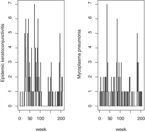
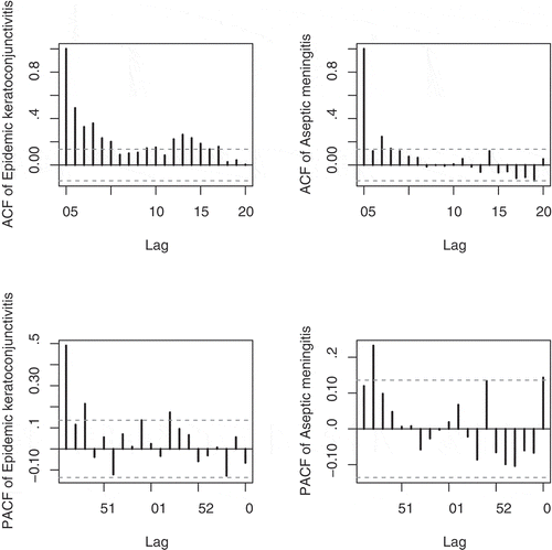
Figure 2 shows the sample ACF and PACF plots for each disease. The figure shows the time dependency but any long-range dependence is not observed, so it is acceptable to fit the MGINAR(1) model.

Figure 2. The sample ACF and PACF for the epidemic keratoconjunctivitis data (left hand side) and aseptic meningitis data (right hand side).

We suppose that the time series count data $\{X_t=(X_t^{(\mathrm{E}\mathrm{K})},X_t^{(\mathrm{A}\mathrm{M})}{)}^{\mathrm{T}}\}$ follows

$X_t=A\circ X_{t-1}+{ϵ}_t$

where both of the thinning operator and the innovation follows the Binomial or Poisson distribution. The CLS estimator (${\hat{a}}_{CLS},{\hat{A}}_{CLS}$) for the parameter ($a,A$) is obtained as follows:

$\left({\hat{a}}_{CLS},{\hat{A}}_{CLS}\right)=\left(\left[\begin{array}{c}0.4050\\ 0.5534\end{array}\right],\left[\begin{array}{cc}0.4845& 0.1240\\ 0.0188& 0.1179\end{array}\right]\right).$

Next, our proposed estimators for the Binomial thinning and the Binomial innovation (${\hat{a}}_{E.B},{\hat{A}}_{E.B}$) and for the Poisson thinning and the Poisson innovation (${\hat{a}}_{E.P},{\hat{\mathit{A}}}_{E.P}$) are obtained as follows:

$\left({\hat{a}}_{E.B},{\hat{\mathit{A}}}_{E.B}\right)=\left(\left[\begin{array}{c}0.1813\\ 0.3404\end{array}\right],\left[\begin{array}{cc}0.5208& 0.1222\\ 0.0338& 0.1664\end{array}\right]\right),$

$\left({\hat{a}}_{E.P},{\hat{\mathit{A}}}_{E.P}\right)=\left(\left[\begin{array}{c}0.1703\\ 0.2575\end{array}\right],\left[\begin{array}{cc}0.4747& 0.0534\\ 0.0191& 0.1207\end{array}\right]\right).$

For both cases of the Binomial distribution and the Poisson distribution, ${\hat{a}}_{CLS}$ is greatly changed by our proposed estimation. In contrast, there is not much change with respect to ${\hat{\mathit{A}}}_{CLS}$.

Finally, we evaluate the goodness of fit for each estimator based on AIC. Denote AIC for an estimator $(\hat{a},\hat{\mathit{A}})$ under the Binomial distribution by $AI{C}_{Bin}(\hat{a},\hat{\mathit{A}})$, and under the Poisson distribution by $AI{C}_{Pois}(\hat{a},\hat{\mathit{A}})$. Then, we obtained

$AI{C}_{Bin}({\hat{a}}_{CLS},{\hat{\mathit{A}}}_{CLS})=794.0651,AI{C}_{Bin}({\hat{a}}_{E.B},{\hat{\mathit{A}}}_{E.B})=718.821$

$AI{C}_{Pois}({\hat{a}}_{CLS},{\hat{\mathit{A}}}_{CLS})=43240.3805,AI{C}_{Pois}({\hat{a}}_{E.P},{\hat{\mathit{A}}}_{E.P})=43081.671$

From the above results, we can see that our proposed estimators take good performance in terms of goodness of fit.

Acknowledgements

We thank the anonymous referees for constructive comments. This work was supported by JSPS KAKENHI, Grant Number JP16K00036.

Additional information

Funding

This work was supported by the JSPS [JP16K00036].

Notes on contributors

Hiroshi Shiraishi

Hiroshi Shiraishi received the BS degree in mathematics in 1998 and the MS and Dr degrees in mathematical science from Waseda University, Japan in 2004 and 2007, respectively. He joined the GE Edison Life Insurance Company, the Prudential Life Insurance Company of Japan and the Hannover-Re Reinsurance Company, in 1998, 2000 and 2005, respectively. His research interests are actuarial science, time series analysis, econometric theory and financial engineering. In particular, he investigates the statistical analysis of discrete-valued time series/the statistical estimation of optimal dividend problems in the field of the actuarial science/the statistical estimation of Hawkes graphs and so on. He is currently an associate professor in the Department of Mathematics, Keio University, Japan. He is a fellowof the Institute of Actuary of Japan (FIAJ).

Appendix

Proof of Theorem 1 The proof is similar to that for Theorem 1 in Drost et al. (2008).

Expansion of the log-likelihood ratio: Let $\mathit{u}=(u_1,\dots ,u_q{)}^{\mathrm{T}}\in {\mathbb{R}}^q\mathrm{\setminus }\{\mathbf{0}\}$ with $q=d+d^{2}p$. Under Assumption (A1), we obtain by Taylor’s theorem,

$log\frac{L_n\left(\theta +\frac{\mathit{u}}{\sqrt{n}}|{\mathit{X}}_{-p},\dots ,{\mathit{X}}_n\right)}{L_n\left(\theta |{\mathit{X}}_{-p},\dots ,{\mathit{X}}_n\right)}={\mathit{u}}^{\mathrm{T}}{S}_n(\theta )-\frac{1}{2}{\mathit{u}}^{\mathrm{T}}{\mathit{J}}_n({\tilde{\theta }}_n)\mathit{u}(7)$

where ${\tilde{\theta }}_n$ is a random point on the line-segment between $\theta$ and $\theta +u/\sqrt{n}$ and

$J_n(\theta )=-\frac{1}{\sqrt{n}}\frac{\mathrm{\partial }}{\mathrm{\partial }{\theta }^{\mathrm{T}}}{S}_n(\theta ).(8)$

Then, we show

• Part 0: auxiliary calculations

• Part 1: ${\mathit{S}}_n(\theta )\stackrel{d}{\to }N(\mathbf{0},\mathit{J})$ under ${\mathbb{P}}_{\nu ,\theta ,F,G}$

• Part 2: ${\mathit{J}}_n(\tilde{\theta })\stackrel{P}{\to }J$ under ${\mathbb{P}}_{\nu ,\theta ,F,G}$

• Part 3: non-singularity of $\mathit{J}$.

In what follows, for simplicity, we write $({\mathit{X}}_s,\dots ,{\mathit{X}}_t):={\mathit{X}}_{s:t}$ and $(x_s,\dots ,x_t):=x_{s:t}$ for $s,t\in \mathbb{Z}$ with $s<t$.

Part 0: We first show that the existence of $\mathit{J}$. To do so, we need to show for each ${\theta }_i,{\theta }_j\in \theta$

${\mathbb{E}}_{\nu ,\theta ,F,G}\left[{\dot{\mathrm{\ell }}}_{{\theta }_i}({\mathit{X}}_{(-p):0};\theta ){\dot{\mathrm{\ell }}}_{{\theta }_j}({\mathit{X}}_{(-p):0};\theta )\right]<\mathrm{\infty }.(9)$

It can be shown by Assumptions (A4) and (A6).□

Part 1: From Equations (3) and (4), it follows that

${\mathbb{E}}_{\nu ,\theta ,F,G}\left[{\dot{\mathrm{\ell }}}_{a_i}({\mathit{X}}_{(t-p):t};\theta )|{\mathit{X}}_{(t-p):(t-1)}\right]={\mathbb{E}}_{\nu ,\theta ,F,G}\left[\frac{\mathrm{\partial }}{\mathrm{\partial }{a}_i}log{F}_{a_i}({ϵ}_{i,t})|{\mathit{X}}_{(t-p):(t-1)}\right]=0$

${\mathbb{E}}_{\nu ,\theta ,F,G}\left[{\dot{\mathrm{\ell }}}_{A_{i,j}^{(k)}}({\mathit{X}}_{(t-p):t};\theta )|{\mathit{X}}_{(t-p):(t-1)}\right]={\mathbb{E}}_{\nu ,\theta ,F,G}\left[\frac{\mathrm{\partial }}{\mathrm{\partial }{A}_{i,j}^{(k)}}log{G}_{A_{i,j}^{(k)}}({\xi }_{i,j,r}^{(k)})|{\mathit{X}}_{(t-p):(t-1)}\right]=0$

since ${ϵ}_{i,t}$ and ${\xi }_{i,j,r}^{(k)}$ are independent of $\{{\mathit{X}}_{t-p},\dots ,{\mathit{X}}_{t-1}\}$. Let $w\in {\mathbb{R}}^q$ and ${\dot{\mathrm{\ell }}}_{\theta }={\left({\dot{\mathrm{\ell }}}_{a_1},\dots ,{\dot{\mathrm{\ell }}}_{a_d},{\dot{\mathrm{\ell }}}_{A_{1,1}^{(1)}},\dots ,{\dot{\mathrm{\ell }}}_{A_{d,d}^{(p)}}\right)}^{\mathrm{T}}$. From the above equations, it follows that

${\mathbb{E}}_{\nu ,\theta ,F,G}\left[w^{\mathrm{T}}{\dot{\mathrm{\ell }}}_{\theta }({\mathit{X}}_{(t-p):t};\theta )|{\mathit{X}}_{(t-p):(t-1)}\right]=0$

and by Part 0, it follows that

${\mathbb{E}}_{\nu ,\theta ,F,G}\left[{\left\{w^{\mathrm{T}}{\dot{\mathrm{\ell }}}_{\theta }({\mathit{X}}_{(t-p):t};\theta )\right\}}^2\right]=w^{\mathrm{T}}\mathit{J}w<\mathrm{\infty }.$

Hence, we have, by Lemma B.1 of Drost et al. (2008),

$\frac{1}{\sqrt{n}}\sum _{t=0}^n\left[w^{\mathrm{T}}{\dot{\mathrm{\ell }}}_{\theta }({\mathit{X}}_{(t-p):t};\theta )\right]\stackrel{d}{\to }{w}^{\mathrm{T}}N(\mathbf{0},J)\mathrm{u}\mathrm{n}\mathrm{d}\mathrm{e}\mathrm{r}{\mathbb{P}}_{\nu ,\theta ,F,G}.$

An application of the Cramér-Wold device concludes the proof of Part 1.□

Part 2: Assumption (A3) implies that, for fixed $x_{-p},\dots ,x_0\in {\mathbb{Z}}_{+}^d$ and for each ${\theta }_i,{\theta }_j\in \mathit{\theta }$, the mapping

$\mathit{\theta }\mapsto (\mathrm{\partial }/\mathrm{\partial }{\theta }_i)log{\dot{\mathrm{\ell }}}_{{\theta }_j}(x_{(-p):0};\mathit{\theta })$

is continuous, respectively. Since we have already proved (9) in Part 0, by Lemma B.3 of Drost et al. (2008), the proof is completed if we have $J_n(\theta )\stackrel{p}{\to }J$ where

${\mathit{J}}_n(\theta )=-\frac{1}{n}\sum _{t=0}^n\left(\begin{array}{cc}\left(\frac{\mathrm{\partial }}{\mathrm{\partial }{a}_i}{\dot{\mathrm{\ell }}}_{a_{i^{\prime }}}({\mathit{X}}_{(t-p):t};\theta )\right)& \left(\frac{\mathrm{\partial }}{\mathrm{\partial }{a}_i}{\dot{\mathrm{\ell }}}_{A_{i^{\prime },j^{\prime }}^{(k^{\prime })}}({\mathit{X}}_{(t-p):t};\theta )\right)\\ \left(\frac{\mathrm{\partial }}{\mathrm{\partial }{A}_{i,j}^{(k)}}{\dot{\mathrm{\ell }}}_{a_{i^{\prime }}}({\mathit{X}}_{(t-p):t};\theta )\right)& \left(\frac{\mathrm{\partial }}{\mathrm{\partial }{A}_{i,j}^{(k)}}{\dot{\mathrm{\ell }}}_{A_{i^{\prime },j^{\prime }}^{(k^{\prime })}}({\mathit{X}}_{(t-p):t};\theta )\right)\\ \hspace{0.17em}& \hspace{0.17em}\end{array}\right).$

For $i,i^{\prime }\in \{1,\dots ,d\}$ and $t\in \{0,1,\dots ,n\}$, it follows that from Equation (3)

$\begin{array}{l}\frac{\partial }{\partial a_i}{\dot{\ell }}_{a_{i^{\prime }}}(x_{(t-p):t};\theta )\\ =\partial \partial a_i\left[\prod _{i^{″}=1}^d\left\{{\tilde{F}}_{i^{\prime },i^{″}}⊛\left(\begin{array}{l}\otimes k=1,\cdots ,p{G}_{A_{i^{″},j}^{(k)}}^{x_{j,t-k^{\otimes }}}\\ j=1,\cdots ,d\end{array}\right)\right\}\left(x_{i^{″}=1}\right)\right]\frac{1_{(0,1}\left(P_{{(x_{t-p},\cdots ,x_{t-1})}^{,x_t}}^{\theta }\right)}{{\left(P_{{(x_{t-p},\cdots ,x_{t-1})}^{,x_t}}^{\theta }\right)}^2}\\ -\left(\partial \partial a_i{P}_{{(x_{t-p},\cdots ,x_{t-1})}^{,x_t}}^{\theta }\right)\prod _{i^{″}=1}^d{\tilde{F}}_{i^{\prime },i^{″}}⊛\left\{{\tilde{F}}_{i^{\prime },i^{″}}⊛\left(\begin{array}{l}\otimes k=1,\cdots ,p{G}_{A_{i^{″},j}^{(k)}}^{x_{j,t-k^{\otimes }}}\\ j=1,\cdots ,d\end{array}\right)\right\}\left(x_{i^{″}=1}\right)\frac{1_{(0,1]}\left(P_{{(x_{t-p},\cdots ,x_{t-1})}^{,x_t}}^{\theta }\right)}{{\left(P_{{(x_{t-p},\cdots ,x_{t-1})}^{,x_t}}^{\theta }\right)}^2}\\ =\prod _{i^{″}=1}^d{\tilde{F}}_{i^{\prime },i^{″}}⊛\left\{{\tilde{F}}_{i^{\prime },i^{″}}⊛\left(\begin{array}{l}\otimes k=1,\cdots ,p{G}_{A_{i^{″},j}^{(k)}}^{x_{j,t-k^{\otimes }}}\\ j=1,\cdots ,d\end{array}\right)\right\}(x_{{i^{\prime }}^{\prime },t})\frac{1_{(0,1}\left(P_{(x_{(t-p):(t-1)}),x_t}^{\theta }\right)}{P_{x_{(t-p):(t-1)},x_t}^{\theta }}\\ -{\dot{\ell }}_{a_i}(x_{(t-p):t};\theta ){\dot{\ell }}_{a_{i^{\prime }}}(x_{(t-p):t};\theta )\\ ={\mathbb{E}}_{\nu ,\theta ,F,G}\left[{\partial }_{a_i,a_{i^{\prime }}}\log F_a\left({ϵ}_t\right)|X_{(t-p):t}=x_{(t-p):t}\right]-{\dot{\ell }}_{a_i}(x_{(t-p):t};\theta ){\dot{\ell }}_{a_{i^{\prime }}}(x_{(t-p):t};\theta )\end{array}$

where

${\tilde{\tilde{F}}}_{i,i^{\prime },i^{″}}=\{\begin{array}{l}{\dot{f}}_{a_i}\text{if}i=i^{\prime }=i^{″}\\ f_{a_i}\text{if}i=i^{″}\ne i^{\prime }\\ f_{a_{i^{\prime }}}\text{if}i\ne i^{\prime }=i^{″}\\ F_{a_{i^{″}}}\text{others}\end{array}$

and

${\mathrm{\partial }}_{a_i,a_{i^{\prime }}}log{F}_a\left({ϵ}_t\right)=\left\{\begin{array}{cc}\frac{{\mathrm{\partial }}^2}{{(\mathrm{\partial }{a}_i)}^2}log{F}_{a_i}\left({ϵ}_{i,t}\right)& \mathrm{i}\mathrm{f}i=i^{\prime }\\ \frac{\mathrm{\partial }}{\mathrm{\partial }{a}_i}log{F}_{a_i}\left({ϵ}_{i,t}\right)\frac{\mathrm{\partial }}{\mathrm{\partial }{a}_{i^{\prime }}}log{F}_{a_{i^{\prime }}}\left({ϵ}_{i^{\prime },t}\right)& \mathrm{i}\mathrm{f}i\ne i^{\prime }\\ \hspace{0.17em}& \hspace{0.17em}\end{array}\right.$

which implies that

${\mathbb{E}}_{\nu ,\theta ,F,G}\left[\frac{\mathrm{\partial }}{\mathrm{\partial }{a}_i}{\dot{\mathrm{\ell }}}_{a_{i^{\prime }}}({\mathit{X}}_{(t-p):t};\theta )\right]={\mathbb{E}}_{\nu ,\theta ,F,G}\left[{\mathbb{E}}_{\nu ,\theta ,F,G}\left[{\mathrm{\partial }}_{a_i,a_{i^{\prime }}}log{F}_a\left({ϵ}_t\right)|{\mathit{X}}_{(t-p):t}\right]-{\dot{\mathrm{\ell }}}_{a_i}({\mathit{X}}_{(t-p):t};\mathit{\theta }){\dot{\mathrm{\ell }}}_{a_{i^{\prime }}}({\mathit{X}}_{(t-p):t};\theta )\right]={\mathbb{E}}_{\nu ,\theta ,F,G}\left[{\mathbb{E}}_{\nu ,\theta ,F,G}\left[{\mathrm{\partial }}_{a_i,a_{i^{\prime }}}log{F}_a\left({ϵ}_t\right)|{\mathit{X}}_{(t-p):(t-1)}\right]\right]-{\mathbb{E}}_{\nu ,\theta ,F,G}\left[{\dot{\mathrm{\ell }}}_{a_i}({\mathit{X}}_{(t-p):t};\theta ){\dot{\mathrm{\ell }}}_{a_{i^{\prime }}}({\mathit{X}}_{(t-p):t};\theta )\right]={\mathbb{E}}_{\nu ,\theta ,F,G}\left[{\mathrm{\partial }}_{a_i,a_{i^{\prime }}}log{F}_a\left({ϵ}_t\right)\right]-J_{a_i,a_{i^{\prime }}}=-J_{a_i,a_{i^{\prime }}}$

where the third equation follows the independence between ${ϵ}_t$ and $X_{(t-p):(t-1)}$. This result and Lemma B.3 of Drost et al. (2008) yield

$-\frac{1}{n}\sum _{t=0}^n\frac{\mathrm{\partial }}{\mathrm{\partial }{a}_i}{\dot{\mathrm{\ell }}}_{a_{i^{\prime }}}({\mathit{X}}_{(t-p):t};\mathit{\theta })\stackrel{p}{\to }-{\mathbb{E}}_{\nu ,\theta ,F,G}\left[\frac{\mathrm{\partial }}{\mathrm{\partial }{a}_i}{\dot{\mathrm{\ell }}}_{a_{i^{\prime }}}({\mathit{X}}_{(-p):0};\mathit{\theta })\right]=J_{a_i,a_{i^{\prime }}}$

By the same argument, we obtain

$\begin{array}{l}-\frac{1}{n}{\displaystyle \sum _{t=0}^n\frac{\partial }{\partial a_i}}{\dot{\ell }}_{A_{i^{\prime },j^{\prime }}^{(k^{\prime })}}(X_{(t-p):t};\theta )\stackrel{p}{\to }{J}_{a_i,A_{i^{\prime },j^{\prime }}^{(k^{\prime })}},-\frac{1}{n}{\displaystyle \sum _{t=0}^n\frac{\partial }{\partial A_{i,j}^{(k)}}}{\dot{\ell }}_{a_{i^{\prime }}}(X_{(t-p):t};\theta )\stackrel{p}{\to }{J}_{A_{i,j}^{(k)},a_{i^{\prime }}},\\ -\frac{1}{n}{\displaystyle \sum _{t=0}^n\frac{\partial }{\partial A_{i,j}^{(k)}}}{\dot{\ell }}_{A_{i^{\prime },j^{\prime }}^{(k^{\prime })}}(X_{(t-p):t};\theta )\stackrel{p}{\to }{J}_{A_{i,j}^{(k)},A_{i^{\prime },j^{\prime }}^{(k^{\prime })}}.\end{array}$

This completes the proof of Part 2.

Part 3: The proof of the non-singularity for $J$ is provided by Assumption (A5) in the same way as Drost et al. (2008).

Proof of Theorem 2 The proof is the same as Theorem 3.2 of Drost et al. (2008).

To calculate the one-step estimator $({\hat{\theta }}_{\ast })$, we need to know the score functions $({\dot{\mathrm{\ell }}}_{a_i})$ and $({\dot{\mathrm{\ell }}}_{A_{i,j}^{(k)}})$ for each distribution. In what follows, we show the derivation of these functions for Cases 1 and 2 in Section 4.

Derivation of the score $\dot{\mathrm{\ell }}$ for the Case 1 For Case 1, the probability functions $G_{A_{i,j}}$ and $F_{a_i}$ are given by

$G_{A_{i,j}}(x)=A_{i,j}^x(1-A_{i,j}{)}^{1-x},F_{a_i}(x)=a_i^x(1-a_i{)}^{1-x}$

for $x\in \{0,1\}$, which implies that the derivatives $g_{A_{i,j}}$ and $f_{a_i}$ are written as

$g_{A_{i,j}}(x)=\left(\frac{x}{A_{i,j}}-\frac{1-x}{1-A_{i,j}}\right)G_{A_{i,j}}(x),f_{a_i}(x)=\left(\frac{x}{a_i}-\frac{1-x}{1-a_i}\right)F_{a_i}(x).$

Let

$\mathrm{B}\mathrm{i}{\mathrm{n}}_{(n,A)}(x)=\left(\begin{array}{c}n\\ \\ x\end{array}\right)A^x(1-A{)}^{n-x},{\mathrm{B}\mathrm{i}\mathrm{n}}_{(n,A)}^{\mathrm{♢}}(x)=\left(\frac{x}{A}-\frac{n-x}{1-A}\right)\mathrm{B}\mathrm{i}{\mathrm{n}}_{(n,A)}(x)$

for $n\in \mathbb{N}$ and $x\in \{0,\dots ,n\}$. Let $\mathrm{B}\mathrm{i}{\mathrm{n}}_{(0,A)}(0)=1,{\mathrm{B}\mathrm{i}\mathrm{n}}_{(0,A)}^{\mathrm{♢}}(0)=0$ and $\mathrm{B}\mathrm{i}{\mathrm{n}}_{(0,A)}(x)={\mathrm{B}\mathrm{i}\mathrm{n}}_{(0,A)}^{\mathrm{♢}}(x)=0$ for $x\ne 0$. Then, we obtain for $i,j=1,2,$

$P_{(x_{t-1}),x_t}^{\theta }=\sum _{(1)}\mathrm{B}\mathrm{i}{\mathrm{n}}_{(1,a_1)}(n_1)\mathrm{B}\mathrm{i}{\mathrm{n}}_{(x_{1,t-1},A_{1,1})}(n_2)\mathrm{B}\mathrm{i}{\mathrm{n}}_{(x_{2,t-1},A_{1,2})}(n_3)\times \sum _{(2)}\mathrm{B}\mathrm{i}{\mathrm{n}}_{(1,a_2)}(n_1^{\prime })\mathrm{B}\mathrm{i}{\mathrm{n}}_{(x_{1,t-1},A_{2,1})}(n_2^{\prime })\mathrm{B}\mathrm{i}{\mathrm{n}}_{(x_{2,t-1},A_{2,2})}(n_3^{\prime }),$

${\dot{\mathrm{\ell }}}_{a_i}(x_{t-1},x_t;\theta )=\sum _{(1)}{\mathrm{B}\mathrm{i}\mathrm{n}}_{(1,a_i)}^{\mathrm{♢}}(n_1)\mathrm{B}\mathrm{i}{\mathrm{n}}_{(x_{1,t-1},A_{i,1})}(n_2)\mathrm{B}\mathrm{i}{\mathrm{n}}_{(x_{2,t-1},A_{i,2})}(n_3)\times \sum _{(2)}\mathrm{B}\mathrm{i}{\mathrm{n}}_{(1,a_{3-i})}(n_1^{\prime })\mathrm{B}\mathrm{i}{\mathrm{n}}_{(x_{1,t-1},A_{3-i,1})}(n_2^{\prime })\mathrm{B}\mathrm{i}{\mathrm{n}}_{(x_{2,t-1},A_{3-i,2})}(n_3^{\prime })/P_{(x_{t-1}),x_t}^{\theta }$

${\dot{\mathrm{\ell }}}_{A_{i,j}}(x_{t-1},x_t;\theta )=\sum _{(1)}\mathrm{B}\mathrm{i}{\mathrm{n}}_{(1,a_i)}(n_1){\mathrm{B}\mathrm{i}\mathrm{n}}_{(x_{j,t-1},A_{i,j})}^{\mathrm{♢}}(n_{j+1})\mathrm{B}\mathrm{i}{\mathrm{n}}_{(x_{3-j,t-1},A_{i,3-j})}(n_{4-j})\times \sum _{(2)}\mathrm{B}\mathrm{i}{\mathrm{n}}_{(1,a_{3-i})}(n_1^{\prime })\mathrm{B}\mathrm{i}{\mathrm{n}}_{(x_{1,t-1},A_{3-i,1})}(n_2^{\prime })\mathrm{B}\mathrm{i}{\mathrm{n}}_{(x_{2,t-1},A_{3-i,2})}(n_3^{\prime })/P_{(x_{t-1}),x_t}^{\theta }$

where ${\sum }_{(1)}={\sum }_{\begin{array}{c}{n}_1+n_2+n_3=x_{i,t},\\ n_1\in \{0,1\},\\ n_2\in \{0,\dots ,x_{1,t-1}\},\\ n_3\in \{0,\dots ,x_{2,t-1}\}\end{array}}$ and ${\sum }_{(2)}={\sum }_{\begin{array}{c}{n^{\prime }}_1+{n^{\prime }}_2+{n^{\prime }}_3=x_{3-i,t},\\ {n^{\prime }}_1\in \{0,1\},\\ {n^{\prime }}_2\in \{0,\dots ,x_{1,t-1}\},\\ {n^{\prime }}_3\in \{0,\dots ,x_{2,t-1}\}\end{array}}$.

The derivation of the score $\dot{\mathrm{\ell }}$ for Case 2 For Case 2, the probability functions $G_{A_{i,j}}$ and $F_{a_i}$ are given by

$G_{A_{i,j}}(x):=(A_{i,j}{)}^{x}exp(-(A_{i,j}))/x!,F_{a_i}(x):=(a_i{)}^{x}exp(-(a_i))/x!$

for $x\in {\mathbb{Z}}_{+}$, which implies that the derivatives $g_{A_{i,j}}$ and $f_{a_i}$ are written by

$g_{A_{i,j}}(x)=\left(\frac{x}{A_{i,j}}-1\right)G_{A_{i,j}}(x),f_{a_i}(x)=\left(\frac{x}{a_i}-1\right)F_{a_i}(x).$

Let

$\mathrm{P}\mathrm{o}\mathrm{i}{\mathrm{s}}_{(\lambda )}(x)=\frac{{\lambda }^x{e}^{-\lambda }}{x!},{\mathrm{P}\mathrm{o}\mathrm{i}\mathrm{s}}_{(\lambda )}^{\mathrm{♢}}(x)=\left(\frac{x}{\lambda }-1\right)\frac{{\lambda }^x{e}^{-\lambda }}{x!}$

and

${\mathrm{P}\mathrm{o}\mathrm{i}\mathrm{s}}_{(nA)}^{\mathrm{♢}\mathrm{♢}}(x)=\left\{\begin{array}{cc}0& \mathrm{i}\mathrm{f}n=0\\ {\mathrm{P}\mathrm{o}\mathrm{i}\mathrm{s}}_{(A)}^{\mathrm{♢}}(x)& \mathrm{i}\mathrm{f}n=1\\ \sum _{x_1+x_2=x}n{\mathrm{P}\mathrm{o}\mathrm{i}\mathrm{s}}_{(A)}^{\mathrm{♢}}(x_1)\mathrm{P}\mathrm{o}\mathrm{i}{\mathrm{s}}_{((n-1)A)}(x_2)& \mathrm{i}\mathrm{f}n>1\\ \hspace{0.17em}& \hspace{0.17em}\end{array}\right.$

for $n\in {\mathbb{Z}}_{+},A>0,x\in {\mathbb{Z}}_{+}$. Then, we obtain for $i,j=1,2,$

$P_{(x_{t-1}),x_t}^{\theta }=\sum _{(3)}\mathrm{P}\mathrm{o}\mathrm{i}{\mathrm{s}}_{(a_1)}(n_1)\mathrm{P}\mathrm{o}\mathrm{i}{\mathrm{s}}_{(x_{1,t-1}{A}_{1,1})}(n_2)\mathrm{P}\mathrm{o}\mathrm{i}{\mathrm{s}}_{(x_{2,t-1}{A}_{1,2})}(n_3)\times \sum _{(4)}\mathrm{P}\mathrm{o}\mathrm{i}{\mathrm{s}}_{(a_2)}(n_1^{\prime })\mathrm{P}\mathrm{o}\mathrm{i}{\mathrm{s}}_{(x_{1,t-1}{A}_{2,1})}(n_2^{\prime })\mathrm{P}\mathrm{o}\mathrm{i}{\mathrm{s}}_{(x_{2,t-1}{A}_{2,2})}(n_3^{\prime })$

${\dot{\mathrm{\ell }}}_{a_i}(x_{t-1},x_t;\theta )=\sum _{(3)}{\mathrm{P}\mathrm{o}\mathrm{i}\mathrm{s}}_{(a_i)}^{\mathrm{♢}}(n_1)\mathrm{P}\mathrm{o}\mathrm{i}{\mathrm{s}}_{(x_{1,t-1}{A}_{i,1})}(n_2)\mathrm{P}\mathrm{o}\mathrm{i}{\mathrm{s}}_{(x_{2,t-1}{A}_{i,2})}(n_3)\times \sum _{(4)}\mathrm{P}\mathrm{o}\mathrm{i}{\mathrm{s}}_{(a_{3-i})}(n_1^{\prime })\mathrm{P}\mathrm{o}\mathrm{i}{\mathrm{s}}_{(x_{1,t-1}{A}_{3-i,1})}(n_2^{\prime })\mathrm{P}\mathrm{o}\mathrm{i}{\mathrm{s}}_{(x_{2,t-1}{A}_{3-i,2})}(n_3^{\prime })/P_{(x_{t-1}),x_t}^{\theta }$

${\dot{\mathrm{\ell }}}_{A_{i,j}}(x_{t-1},x_t;\theta )=\sum _{(3)}\mathrm{P}\mathrm{o}\mathrm{i}{\mathrm{s}}_{(a_i)}(n_1){\mathrm{P}\mathrm{o}\mathrm{i}\mathrm{s}}_{(x_{j,t-1}{A}_{i,j})}^{\mathrm{♢}\mathrm{♢}}(n_{j+1})\mathrm{P}\mathrm{o}\mathrm{i}{\mathrm{s}}_{(x_{3-j,t-1}{A}_{i,3-j})}(n_{4-j})\times \sum _{(4)}\mathrm{P}\mathrm{o}\mathrm{i}{\mathrm{s}}_{(a_{3-i})}(n_1^{\prime })\mathrm{P}\mathrm{o}\mathrm{i}{\mathrm{s}}_{(x_{1,t-1}{A}_{3-i,1})}(n_2^{\prime })\mathrm{P}\mathrm{o}\mathrm{i}{\mathrm{s}}_{(x_{2,t-1}{A}_{3-i,2})}(n_3^{\prime })/P_{(x_{t-1}),x_t}^{\theta }$

where ${\sum }_{(3)}={\sum }_{\genfrac{}{}{0ex}{}{n_1+n_2+n_3=x_{i,t},}{n_1,n_2,n_3\in \{0,\dots ,x_{i,t}\}}}$ and ${\sum }_{(4)}={\sum }_{\genfrac{}{}{0ex}{}{{n^{\prime }}_1+{n^{\prime }}_2+{n^{\prime }}_3=x_{3-i,t},}{{n^{\prime }}_1,{n^{\prime }}_2,{n^{\prime }}_3\in \{0,\dots ,x_{3-i,t}\}}}$□

References

- Al-Osh, M. A., & Alzaid, A. A. (1987). First-order integer-valued autoregressive (INAR(1)) process. Journal of Time Series Analysis, 8(3), 261–18. doi:10.1111/j.1467-9892.1987.tb00438.x
- Alzaid, A. A., & Al-Osh, M. A. (1990). An integer-valued pth-order autoregressive structure (INAR(p)) process. Journal of Applied Probability, 27(2), 314–324. doi:10.2307/3214650
- Bu, R., McCabe, B., & Hadri, K. (2008). Maximum likelihood estimation of higher-order integer-valued autoregressive processes. Journal of Time Series Analysis, 29(6), 973–994. doi:10.1111/j.1467-9892.2008.00590.x
- Cox, D. R., & Hinkley, D. (1974). Theoretical statistics. London: Chapman and Hall.
- Drost, F. C., Van Den Akker, R., & Werker, B. J. M. (2008). Local asymptotic normality and efficient estimation for INAR (p) models. Journal of Time Series Analysis, 29(5), 783–801. doi:10.1111/j.1467-9892.2008.00581.x
- Du, J. G., & Li, Y. (1991). The integer-valued autoregressive (INAR(p)) model. Journal of Time Series Analysis, 12(2), 129–142. doi:10.1111/j.1467-9892.1991.tb00073.x
- Franke, J., & Subba Rao, T. 1993. Multivariate first-order integer-valued autoregression. Technical report No.95, Universität Kaiserslautern.
- Karlis, D., & Pedeli, X. (2013). Flexible bivariate INAR(1) processes using copulas. Communications in Statistics-Theory and Methods, 42(4), 723–740. doi:10.1080/03610926.2012.754466
- Latour, A. (1997). The multivariate GINAR(p) process. Advances in Applied Probability, 29(1), 228–248. doi:10.2307/1427868
- Latour, A. (1998). Existence and stochastic structure of a non-negative integer-valued autoregressive process. Journal of Time Series Analysis, 19(4), 439–455. doi:10.1111/jtsa.1998.19.issue-4
- McKenzie, E. (1985). Some simple models for discrete variate time series. Water Resources Bulletin, 21(4), 645–650. doi:10.1111/j.1752-1688.1985.tb05379.x
- McKenzie, E. (1988). Some ARMA models for dependent sequences of Poisson counts. Advances in Applied Probability, 20(4), 822–835. doi:10.2307/1427362
- Ristić, M. M., Bakouch, H. S., & Nastić, A. S. (2009). A new geometric first-order integer-valued autoregressive (NGINAR(1)) process. Journal of Statistical Planning and Inference, 139(7), 2218–2226. doi:10.1016/j.jspi.2008.10.007
- Serfling, R. (2011). Asymptotic relative efficiency in estimation. In M. Lovric (Ed.), International encyclopedia of statistical science, (pp. 68–82). Berlin, Heidelberg: Springer.
- Weiß, C. H. (2018). An introduction to discrete-valued time series. Chichester: John Wiley & Sons.