On a symbolic method for neutral functional-differential equations with proportional delays

Abstract

In this paper, we present a new symbolic method for solving neutral functional-differential equations with proportional delays having variable coefficients via homotopy perturbation method. The proposed symbolic method is also applicable to solve the multi-pantograph equations with variable coefficients. Several numerical examples are given to illustrate the proposed method and the results show that the proposed symbolic method is very effective.

Keywords:

• multi-pantograph equations
• neutral functional-differential equations
• homotopy perturbation method
• symbolic method

PUBLIC INTEREST STATEMENT

Functional-differential equations (FDEs) and multi-pantograph equations (MPEs) are playing an important role in the mathematical modeling of real-world phenomena. FDEs find use in mathematical models that assume a specified behavior or phenomenon depends on the present as well as the past state of a system. In other words, past events explicitly influence future results. For this reason, FDEs are used to in many applications rather than ordinary differential equations, in which future behavior only implicitly depends on the past. FDEs and the MPEs arise in many applications, such as number theory, probability theory on algebraic structures, electrodynamics, astrophysics, non-linear dynamical systems, quantum mechanics, cell growth, etc.

1. Introduction

Functional-differential equations are playing an important role in the mathematical modeling of real-world phenomena and the multi-pantograph equations arise in many applications, such as number theory, probability theory on algebraic structures, electrodynamics, astrophysics, non-linear dynamical systems, quantum mechanics,and cell growth, etc., these equations cannot be solved by one of the known standard methods. Functional-differential equations find use in mathematical models that assume a specified behavior or phenomenon depends on the present as well as the past state of a system. In other words, past events explicitly influence future results. For this reason, Functional-differential equations are used to in many applications rather than ordinary differential equations, in which future behavior only implicitly depends on the past. Properties of the analytic solution of these equations as well as numerical methods have been studied by several authors, see, for example (Chen & Wang:, 2010; Derfel & Vogl, 1996; Feldstein & Liu, 1998; Sezer et al., 2008).

In this paper, we focus on a new symbolic method to obtain an analytic or approximate solution of a given neutral functional-differential equations in easy and efficient manner. The main idea is that, we follow, similar to the symbolic methods for differential equations discussed in (Thota, 2019; Thota & Kumar, 2016, 2015; Thota & Kumar, 2016a, 2016b, 2015, 2017; Thota et al., 2012; Thota, 2017, 2019a, 2018a, 2018b, 2018c, 2018d, 2019b) to present the proposed method symbolically. Indeed, in this paper, we propose a new symbolic method for finding an analytic or approximate solution of neutral functional-differential equations as well as the multi-pantograph equations with variable coefficients by using the concept of homotopy perturbation method (HPM). The approach to analytic solution of this method is easy and computationally very attractive.

The HPM was introduced first by Dr. He in 1998 (He, 1999; He, 2000). This HPM is one of the a powerful and efficient techniques to find the solutions of the given non-linear equations without using a linearization process. This method is based on a combination of the perturbation and homotopy methods. HPM can take the advantages of the conventional perturbation method while eliminating its restrictions. Many engineers, scientists, and researchers have been applied successfully this method to solve several kinds of non-linear and linear equations in science and engineering (Biazar & Ghazvini, 2008; He, 1999, 2019, 2004; He, 2000; He & Ain, 2020; He & Jin, 2020; Shang, 2012). For example, in (He, 2019), the authors discussed the simpler, the better: Analytical methods for nonlinear oscillators and fractional oscillators; in (Shang, 2012), authors presented a Lie algebra approach to susceptible-infected-susceptible epidemics, Lie algebraic discussion for affinity-based information diffusion in social networks, analytical solution for an in-host viral infection model with time-inhomogeneous rates; in (Biazar & Ghazvini, 2008), new promises and future challenges of fractal calculus: From two-scale thermodynamics to fractal variational principle are presented; and in (He & Jin, 2020) the authors focused a short review on analytical methods for the capillary oscillator in a nanoscale deformable tube.

The main objective of this paper is to present a new easy and efficient symbolic method to obtain an analytic or approximate solution of a given neutral functional-differential equation. In detail, we propose a symbolic method to find an analytic or approximate solution of a given neutral functional-differential equations as well as the multi-pantograph equations with variable coefficients by using the concept of HPM. In this paper, we concern with the neutral functional-differential equation with proportional delays (Jafari & Aminataei, 2012) of the following form

(1) $\begin{array}{cc}\hspace{0.17em}& {(y(x)+\beta (x)y(q_{n}x))}^{(n)}=\lambda y(x)+\sum _{j=0}^{n-1}{\mu }_j(x)y^{(j)}(q_{j}x)+f(x),x\ge 0,\\ \hspace{0.17em}& y^{(i)}(0)=c_i,i=0,1,\dots ,n-1.\end{array}$(1)

where $\lambda ,c_0,c_1,\dots ,c_{n-1}\in \mathbb{C}$; ${\mu }_j(x)$ and $f(x)$ are analytic functions; $0<q_1<\cdots <q_{n-1}\le 1$, and the superscripts indicate differentiation. In order to propose a new method, we rewrite equation (1)(1) $\begin{array}{cc}\hspace{0.17em}& {(y(x)+\beta (x)y(q_{n}x))}^{(n)}=\lambda y(x)+\sum _{j=0}^{n-1}{\mu }_j(x)y^{(j)}(q_{j}x)+f(x),x\ge 0,\\ \hspace{0.17em}& y^{(i)}(0)=c_i,i=0,1,\dots ,n-1.\end{array}$(1) as

(2) $\begin{array}{cc}\hspace{0.17em}& y^{(n)}(x)=\lambda y(x)-{(\beta (x)y(q_{n}x))}^{(n)}+\sum _{j=0}^{n-1}{\mu }_j(x)y^{(j)}(q_{j}x)+f(x),x\ge 0,\\ \hspace{0.17em}& y^{(i)}(0)=c_i,i=0,1,\dots ,n-1.\end{array}$(2)

The multi-pantograph equation is a kind of delay differential equations of the form

(3) $\begin{array}{cc}\hspace{0.17em}& y^{\prime }(x)=\lambda y(x)+\sum _{i=1}^n{\mu }_i(x)y(q_{i}x)+f(x),x\ge 0,\\ \hspace{0.17em}& y(0)=c_0.\end{array}$(3)

Since we are interested to find an analytical or approximate solution of the given neutral functional-differential equations with proportional delays as well as the multi-pantograph equations with variable coefficients in symbolic manner, we use a powerful and efficient method namely HPM. This method is coupling of the homotopy method, a basic concept of topology, and the classical perturbation technique, provides us with a suitable way to obtain approximate or analytic solution for wide variety of problems arising in different fields. One of the advantages of this HPM is, good approximate solutions can be obtained with only a few iterations and HPM yields a very rapid convergence of the solution series in most cases, and another advantage of HPM is that the perturbation equation can be freely constructed in many ways by homotopy in topology and the initial approximation can also be freely selected. In Section 2 we describe the symbolic formulation of the proposed method. Several examples are given in Section 3 to illustrate the efficiency of the symbolic method, and comparisons are made to confirm the reliability of the symbolic method.

1.1. Basic ideas of homotopy perturbation method

In this section, we recall the basic ideas of the HPM, see, for example (He, 1999; He, 2000; Shakeri & Dehghan, 2008) for more details. Consider the following non-linear differential equation:

(4) $L(y)=f(x),x\in \mathcal{S},$(4)

with the initial conditions

(5) $I_c(y,y^{\prime })=0,x\in \mathrm{\Omega },$(5)

where $L$ is a differential operator, $I_c$ is a initial condition operator, $\mathrm{\Omega }$ is the set of initial conditions of the domain $\mathcal{S}$, and $f(x)$ is a forcing analytical function. One can divide the differential operator $L$ into two parts $L_l$ and $L_n$, where $L_l$ is a linear operator and $L_n$ ia a non-linear operator. Now the equation (4)(4) $L(y)=f(x),x\in \mathcal{S},$(4) can be written as

(6) $L_l(y)+L_n(y)=f(x).$(6)

Using HPM, we can construct a homotopy $v(x,p):\mathcal{S}\times [0,1]\to R$ which satisfies, for $p\in [0,1],x\in \mathcal{S}$,

(7) $H(v,p)=(1-p)[L_l(v)-L_l(y_0)]+p[L(v)-f(x)]=0,$(7)

(8) $=L_l(v)-L_l(y_0)+p{L}_l(y_0)+p[L_n(v)-f(x)]=0,$(8)

where $y_0$ is an initial approximation and $p$ is an embedding parameter. One can easily observe that $H(v,0)=L_l(v)-L_l(y_0)=0$ and $H(v,1)=L(v)-f(x)=0$. According to the HPM, we can take the parameter $p$ as a small, and assume that the solution of (7) and (8) can be written as a power series in $p$

$v=\sum _{n=0}^{\mathrm{\infty }}{p}^n{v}_n.$

Setting $p=1$, the approximate solution of non-linear differential equation (4)(4) $L(y)=f(x),x\in \mathcal{S},$(4) is

$y=\underset{p\to 1}{lim}v=\sum _{n=0}^{\mathrm{\infty }}{v}_n.$

In the following section, we present the proposed method.

2. Symbolic formulation

In this section, we illustrate the basic idea of the proposed method to find the solution of the neutral functional-differential equations corresponding to the special choice of $\mathcal{S}=C^{\mathrm{\infty }}[0,1]$ for simplicity. Recall equation (2)(2) $\begin{array}{cc}\hspace{0.17em}& y^{(n)}(x)=\lambda y(x)-{(\beta (x)y(q_{n}x))}^{(n)}+\sum _{j=0}^{n-1}{\mu }_j(x)y^{(j)}(q_{j}x)+f(x),x\ge 0,\\ \hspace{0.17em}& y^{(i)}(0)=c_i,i=0,1,\dots ,n-1.\end{array}$(2) as follows:

(9) $\begin{array}{cc}\hspace{0.17em}& L(y(x)+\beta (x)y(q_{n}x))=\lambda y(x)+\sum _{j=0}^{n-1}{\mu }_j(x)y^{(j)}(q_{j}x)+f(x),\\ \hspace{0.17em}& y(0)=c_0,\mathrm{D}y(0)=c_1,{\mathrm{D}}^{2}y(0)=c_2,\dots ,{\mathrm{D}}^{(n-1)}y(0)=c_{n-1},\end{array}$(9)

where $L:\mathcal{S}\to \mathcal{S}$ is a linear differential operator, i.e., $L={\mathrm{D}}^n=\frac{d^n}{d{x}^n}$, $y\in \mathcal{S}$, and $c_0,\dots ,c_{n-1}$ are constants of $\mathbb{C}$. Analytically speaking, the differential operator $L$ acts on the Banach space ($C[0,1],\parallel \cdot {\parallel }_{\mathrm{\infty }}$) with dense domain of definition $C^n[0,1]$ and algebraically speaking, the domain of $L$ is the complex vector space $C^{\mathrm{\infty }}[0,1]$ without any prescribed topology.

The solution of the fully non-homogeneous neutral functional-differential equations with proportional delays (FDEs) (2) can be divided into the solution of semi non-homogeneous FDEs, i.e., the solution of

(10) $\begin{array}{cc}\hspace{0.17em}& y^{(n)}(x)=\lambda y(x)-{(\beta (x)y(q_{n}x))}^{(n)}+\sum _{j=0}^{n-1}{\mu }_j(x)y^{(j)}(q_{j}x)+f(x),x\ge 0,\\ \hspace{0.17em}& y^{(i)}(0)=0,i=0,1,\dots ,n-1,\end{array}$(10)

and the solution of semi homogeneous FDEs, i.e., the solution of

(11) $\begin{array}{cc}\hspace{0.17em}& y^{(n)}(x)=0,\\ \hspace{0.17em}& y^{(i)}(0)=c_i,i=0,1,\dots ,n-1.\end{array}$(11)

The solution of the semi non-homogeneous FDEs (10) is obtained using the variation of parameters formula (see (Coddington & Levinson, 1955; Thota, 2019; Thota & Kumar, 2016, 2015; Thota & Kumar, 2016a, 2016b, 2015, 2017; Thota et al., 2012; Thota, 2017, 2019a)) and the solution of semi homogeneous FDEs (11) is obtained using the interpolation technique (see (Thota, 2019; Thota & Kumar, 2015; Thota & Kumar, 2016a, 2015, 2017; Thota, 2017, 2019a, 2018a, 2018b, 2018c, 2018d, 2019b)). The solution of the semi non-homogeneous FDEs is computed as follows: Since the solution of (10) involves integration, we introduce an operator $\mathrm{I}$, called integral operator, for computing the antiderivative as follows:

$\mathrm{I}f(x)={\int }_0^{x}f(\xi )d\xi ,$

and $\mathrm{D}\mathrm{I}f=f$, i.e., $\mathrm{D}\mathrm{I}=1$, the operator $\mathrm{I}$ is called the right inverse of $\mathrm{D}$. The powers of integral operator $\mathrm{I}$ can be defined in the obvious way. Of course, every ${\mathrm{I}}^{n}f$ must be continuous. In particular,

$\mathrm{O}\mathrm{A}\mathrm{M}\mathrm{A}\mathrm{\_}\mathrm{A}\mathrm{\_}1813961$

From replacement lemma (Collins, 2006), we have

(12) ${\mathrm{I}}^{2}f(x)=x{\int }_0^{x}f(\xi )d\xi -{\int }_0^x\xi f(\xi )d\xi .$(12)

Thus, equation (12)(12) ${\mathrm{I}}^{2}f(x)=x{\int }_0^{x}f(\xi )d\xi -{\int }_0^x\xi f(\xi )d\xi .$(12) can be written in terms of $I$ as follows

${\mathrm{I}}^{2}f(x)=x\mathrm{I}f(x)-\mathrm{I}xf(x),$

and as an operator we have ${\mathrm{I}}^2=x\mathrm{I}-\mathrm{I}x$. We can easily check that ${\mathrm{D}}^2{\mathrm{I}}^2=1$ and also ${\mathrm{D}}^2(x\mathrm{I}-\mathrm{I}x)=1$. The operator $x\mathrm{I}-\mathrm{I}x$ is called the normal form of ${\mathrm{I}}^2$. Now replacement lemma can be restated in operator-based notations as follows:

Lemma 2.1. If $f(x)$ is integrable, then $I^{2}f(x)=xIf(x)-Ixf(x)$ for all $x\in [0,1]$.

Proof. Result easily follows from the integration by parts as $\mathrm{I}xf(x)=x\mathrm{I}f(x)-{\mathrm{I}}^{2}f(x)$.

Since $D^n{I}^n=1$, $I^n$ is the right inverse of $L=D^n$, and by Lemma 2.1, one can easily compute the normal form of $I^n$ by induction on $n$. Let the normal form of right inverse, $I^n$, be denoted by $L^{†}$ and then $L{L}^{†}=1$. We can also compute the normal form of the right inverse of the differential operator $L$ by using the variation of parameters formula (see (Coddington & Levinson, 1955)) as follows:

Lemma 2.2. For a given differential operator $L=D^n$ with the fundamental system $1,x,x^2,\dots ,x^{n-1}$, the normal form of the right inverse of $L$ is given by

(13) $L^{†}=\sum _{i=1}^n\frac{x^{i-1}}{1!2!\cdots (n-1)!}Idet(W_i),$(13)

where $I$ is the integral operator, i.e., $If={\int }_0^{x}fdx$, $W_i$ is the Wronskian matrix associated with $1,x,\dots ,x^{n-1}$ whose $i$-th column is the $n$-th unit vector.

The solution of the semi homogeneous FDEs is computed as follows: It is clear that the solution of the semi non-homogeneous FDEs (see, e.g. (Thota, 2019; Thota & Kumar, 2016, 2015; Thota & Kumar, 2016a, 2016b, 2015, 2017; Thota et al., 2012; Thota, 2017, 2019a)) depends on the interpolation technique. Indeed, to compute the solution of the IVP (11), it is enough to compute the interpolating function which is satisfying the initial data. Therefore the solution is

$y(x)=\sum _{i=0}^{n-1}{c}_i\frac{x^i}{i!}.$

Now the symbolic formulation of the solution of (9) in terms of normal form is given by,

(14) $y(x)=\varphi +L^{†}g(x,y,y^{\prime },\dots ,y^{(n-1)}),$(14)

where $\varphi =-\beta (x)y(q_{n}x)+{\sum }_{i=0}^{n-1}{c}_i\frac{x^i}{i!}$; $L^{†}$ is the right inverse of the differential operator $L$ as given in the Lemma 2.2; and $g(x,y,y^{\prime },\dots ,y^{(n-1)})=\lambda y(x)+{\sum }_{j=0}^{n-1}{\mu }_j(x)y^{(j)}(q_{j}x)+f(x)$.

As mentioned, in introduction, that one of the advantages of HPM is that the perturbation equation can be freely constructed in many ways by homotopy in topology and the initial approximation can also be freely selected. Here, we are going to discuss two ways to construct the perturbation equation. One way to construct the perturbation equation is as follows.

According to HPM (He, 1999; He, 2000), we can write the solution (14) as a power series in $p$,

(15) $v=\sum _{n=0}^{\mathrm{\infty }}{p}^n{v}_n.$(15)

Setting $p=1$, the approximate solution of equation (15)(15) $v=\sum _{n=0}^{\mathrm{\infty }}{p}^n{v}_n.$(15) is

(16) $y=\underset{p\to 1}{lim}v=\sum _{n=0}^{\mathrm{\infty }}{v}_n.$(16)

To solve the given equation (1)(1) $\begin{array}{cc}\hspace{0.17em}& {(y(x)+\beta (x)y(q_{n}x))}^{(n)}=\lambda y(x)+\sum _{j=0}^{n-1}{\mu }_j(x)y^{(j)}(q_{j}x)+f(x),x\ge 0,\\ \hspace{0.17em}& y^{(i)}(0)=c_i,i=0,1,\dots ,n-1.\end{array}$(1) using HPM, we have the convex homotopy from equation (7)(7) $H(v,p)=(1-p)[L_l(v)-L_l(y_0)]+p[L(v)-f(x)]=0,$(7) as follows:

(17) $\begin{array}{cc}H(v,p)=& (1-p)[v^{(n)}(x)-y_0^{(n)}(x)]+p[v^{(n)}(x)-\lambda v(x)+\beta (x)v^{(n)}(q_{n}x)\\ \hspace{0.17em}& -\sum _{j=0}^{n-1}{\mu }_j(x)v^{(j)}(q_{j}x)-f(x)]=0.\end{array}$(17)

Substituting (15) in (17) and equating the coefficients of powers of $p$, yield

$p^0:v_0^{(n)}(x)-y_0^{(n)}(x)=0,v_0^{(i)}(0)=c_i,i=0,1,\dots ,n-1,$

$p^1:v_1^{(n)}(x)+y_0^{(n)}(x)-\lambda y_0(x)+\beta (x)y_0^{(n)}(q_{n}x)-\sum _{j=0}^{n-1}{\mu }_j(x)y_0^{(j)}(q_{j}x),$

$v_1^{(i)}(0)=0,i=0,1,\dots ,n-1,$

$⋮$

$p^k:v_k^{(n)}(x)+\beta (x)y_{k-1}^{(n)}(q_{n}x)-\lambda y_{k-1}(x)-\sum _{j=0}^{n-1}{\mu }_j(x)y_{k-1}^{(j)}(q_{j}x),$

$v_k^{(i)}(0)=0,i=0,1,\dots ,n-1.$

Identifying the components $v_i$’s, the $n$th approximation of the exact solution can be obtained as

$y_n=\sum _{i=0}^n{v}_i.$

Another way to construct the perturbation equation is as follows.

Using the HPM, we can construct the following homotopy for the equation (1)(1) $\begin{array}{cc}\hspace{0.17em}& {(y(x)+\beta (x)y(q_{n}x))}^{(n)}=\lambda y(x)+\sum _{j=0}^{n-1}{\mu }_j(x)y^{(j)}(q_{j}x)+f(x),x\ge 0,\\ \hspace{0.17em}& y^{(i)}(0)=c_i,i=0,1,\dots ,n-1.\end{array}$(1) . The functions $v_n$, for $n=0,1,\dots$, are determined as follows (see, e.g. (He, 1999), (He, 2000)):

(18) $\sum _{n=0}^{\mathrm{\infty }}{p}^n{v}_n=\varphi +p\left(L^{†}\sum _{n=0}^{\mathrm{\infty }}{p}^n{v}_n\right).$(18)

The functions $v_n$ are obtained by equating the corresponding coefficient of power of $p$ on both sides, for $n=1,2,3,\dots$,

(19) $\begin{array}{cc}{p}^0:v_0=& \varphi \\ p^n:v_n=& L^{†}{v}_{n-1}.\end{array}$(19)

Here, we are mainly concerned about the perturbation equation that can be constructed easily in many ways by homotopy, and the initial guess that can also be selected freely by HPM. Once one chooses these parts, the homotopy equation is completely determined, because the remaining part is actually the original equation and we have less freedom to change it.

Remark: This theory can also be easily extended to fractal calculus.

2.1. Error involving due to approximation

If $y_k(x)$ is an approximate solution at level $n=k$, then the error involved due to the approximation is calculated as follows and it must be approximately zero, for $i=0,1,\dots$,

$E_k(x_i)=|y(x_i)-y_k(x_i)|\stackrel{\approx }{\text{relbar}\phantom{{ }_{\text{vbox}to.5ex\text{vss}}}}0$

or

$E_k(x_i)=\begin{array}{c}{(y_k(x_i)+\beta (x_i)y_k(q_n{x}_i))}^{(n)}-\lambda y_k(x_i)-{\sum }_{j=0}^{n-1}{\mu }_j(x_i)y_k^{(j)}(q_j{x}_i)+f(x_i)\end{array}\stackrel{\approx }{\text{relbar}\phantom{{ }_{\text{vbox}to.5ex\text{vss}}}}0.$

In the following section, we present several numerical examples to illustrate the simplicity and efficiency of the proposed method.

3. Numerical examples

Example 3.1. Consider the following multi-pantograph equation

(20) $\begin{array}{cc}\hspace{0.17em}& y^{\prime }(x)=\lambda y(x)+\mu y(\frac{x}{2}),\\ \hspace{0.17em}& y(0)=1,0\le x\le 1.\end{array}$(20)

where $\lambda =\frac{a}{2}$ and $\mu =\frac{a}{2}{e}^{\frac{ax}{2}}$. In symbolic notations, we have $Ly(x)=f(x,y)$ where $L=D$, $f(x,y)=\frac{a}{2}{e}^{\frac{ax}{2}}y(\frac{x}{2})+\frac{a}{2}y(x)$ and $c_0=1$. The right inverse of $L$, computed as discussed in Section 2, is $L^{†}=I$.

By HPM, we have the following convex homotopy

(21) $\sum _{n=0}^{\mathrm{\infty }}{p}^n{y}_n=c_0+p\left(L^{†}\sum _{n=0}^{\mathrm{\infty }}{p}^n\left(\lambda y_n(x)+\mu y_n(\frac{x}{2})\right)\right).$(21)

Comparing the corresponding coefficient of power of $p$ on both sides, for $n=1,2,3,\dots$,

$\begin{array}{cc}{p}^0:y_0=& c_0=1,\\ \\ p^1:y_1=& L^{†}\left(\lambda y_0(x)+\mu y_0(\frac{x}{2})\right)=\frac{a}{2}x+e^{\frac{ax}{2}}-1,\\ \\ p^2:y_2=& L^{†}\left(\lambda y_1(x)+\mu y_1(\frac{x}{2})\right)=-\frac{1}{6}-\frac{ax}{2}+\frac{x^2{a}^2}{8}+\frac{2}{3}{e}^{\frac{3ax}{4}}+\frac{ax-2}{4}{e}^{\frac{ax}{2}},\\ \\ p^3:y_3=& \frac{1}{28}+\frac{8}{21}{e}^{\frac{7ax}{8}}-\frac{x^2{a}^2}{8}+\frac{x^3{a}^3}{48}+\frac{1}{96}(3x^2{a}^2-40-12ax)e^{\frac{ax}{2}}+\frac{ax}{12}\left(e^{\frac{3ax}{4}-1}\right),\end{array}$

and so on, in this manner the rest of components of the homotopy perturbation solution can be obtained. Now we can approximate the analytical solution $y(x)$ by truncated series as

$y(x)=\sum _{i=0}^n{y}_n\to e^{ax}\mathrm{a}\mathrm{s}n\to \mathrm{\infty }.$

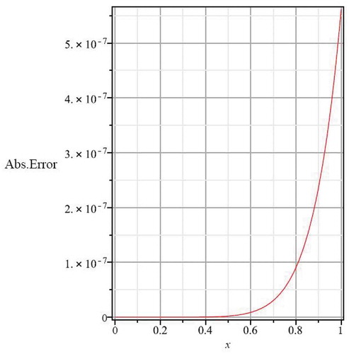
Figure 1 shows the graphical comparison between the exact solution and the approximate solution obtained by the proposed method for $a=1$. It can be seen that the solution obtained by the present method nearly identical to the exact solution. The simplicity and accuracy of the proposed method is illustrated by computing the absolute error $E_7=|y_{exact}(x)-y_{appox}(x)|$. Figure 2 shows the absolute error between the exact and approximate solution at level $n=7$ which is significantly small; thus, it indicates the convergence of series solution very rapidly. The accuracy of the results can be improved by introducing more terms of the approximate solutions. In Table 1, the solution is compared with the well-known exact solution of the given equation (20)(20) $\begin{array}{cc}\hspace{0.17em}& y^{\prime }(x)=\lambda y(x)+\mu y(\frac{x}{2}),\\ \hspace{0.17em}& y(0)=1,0\le x\le 1.\end{array}$(20) . From the numerical results in Table 1, it is clear that the approximate solution is in high agreement with the exact solution. The table also shows the absolute error between the exact solution and approximate solution. The convergence rate of the solution series is very fast.

Figure 1. Graphical results for Example, 3.1.

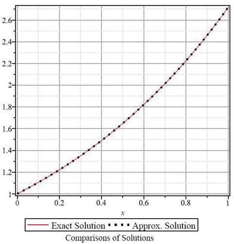
Figure 2. The absolute error $E_7$ for Example, 3.1.

Example 3.2. Consider a second-order neutral functional-differential equation with proposed delay

(22) $\begin{array}{cc}{y}^{\prime \prime }(x)=& y^{\prime }(\frac{x}{2})-\frac{x}{2}{y}^{\prime \prime }(\frac{x}{2})+2,x\in [0,1]\\ y(0)=& 1,y^{\prime }(0)=0.\end{array}$(22)

In symbolic notations, we have $Ly=f(x,y)$ where $L=D^2$, $f(x,y)=y^{\prime }(\frac{x}{2})-\frac{x}{2}{y}^{\prime \prime }(\frac{x}{2})+2$ and $c_0=1,c_1=0$. The right inverse of $L$ is $L^{†}=xI-Ix$. The symbolic representation of (22) is

(23) $y=1+(xI-Ix)\left(y^{\prime }(\frac{x}{2})-\frac{x}{2}{y}^{\prime \prime }(\frac{x}{2})+2\right)$(23)

Now applying the HPM, we have the following convex homotopy

(24) $\sum _{n=0}^{\mathrm{\infty }}{p}^n{y}_n=1+p\left((xI-Ix)\sum _{n=0}^{\mathrm{\infty }}{p}^n{y^{\prime }}_n(\frac{x}{2})-\frac{x}{2}{y}_{n^{\prime \prime }}(\frac{x}{2})+2\right).$(24)

Comparing the corresponding coefficient of power of $p$ on both sides in equation (24)(24) $\sum _{n=0}^{\mathrm{\infty }}{p}^n{y}_n=1+p\left((xI-Ix)\sum _{n=0}^{\mathrm{\infty }}{p}^n{y^{\prime }}_n(\frac{x}{2})-\frac{x}{2}{y}_{n^{\prime \prime }}(\frac{x}{2})+2\right).$(24) , we have, for $n=1,2,3,\dots$,

$\begin{array}{cc}{p}^0:y_0=& 1,\\ \\ p^1:y_1=& (xI-Ix)\left({y^{\prime }}_0(\frac{x}{2})-\frac{x}{2}{y}_{0^{\prime \prime }}(\frac{x}{2})+2\right)=x^2,\\ \\ p^2:y_2=& (xI-Ix)\left({y^{\prime }}_1(\frac{x}{2})-\frac{x}{2}{y}_{1^{\prime \prime }}(\frac{x}{2})+2\right)=x^2,\\ \\ p^3:y_3=& x^2,\\ \\ p^4:y_4=& x^2,\\ \hspace{0.17em}& \hspace{0.17em}\end{array}$

Now we approximate the analytical solution $y(x)$ by truncated series as

$y(x)=\sum _{i=0}^n{y}_n=1+\sum _{i=1}^n{x}^2\to 1+x^2\mathrm{a}\mathrm{s}n\to \mathrm{\infty },$

which is coincides with the exact solution.

Example 3.3. Now consider a third-order neutral functional-differential equation with proposed delay

(25) $\begin{array}{cc}{y}^{\prime \prime \prime }(x)=& y(x)+y^{\prime }(\frac{x}{2})+y^{\prime \prime }(\frac{x}{3})+\frac{1}{2}{y}^{\prime \prime \prime }(\frac{x}{4})\\ \hspace{0.17em}& -x^4-\frac{x^3}{2}-\frac{4x^2}{3}+21x,x\in [0,1]\\ y(0)=& y^{\prime }(0)=y^{\prime \prime }(0)=0.\end{array}$(25)

In symbolic representation, $Ly=f(x,y)$ where $L=D^3$, $f(x,y)=y(x)+y^{\prime }(\frac{x}{2})+y^{\prime \prime }(\frac{x}{3})+\frac{1}{2}{y}^{\prime \prime \prime }(\frac{x}{4})-x^4-\frac{x^3}{2}-\frac{4x^2}{3}+21x$ and $c_0=c_1=c_2=0$. We have the right inverse is $L^{†}=-xIx+\frac{x^2}{2}I+I\frac{x^2}{2}$. The symbolic representation of (25) is

(26) $y=\left(-xIx+\frac{x^2}{2}I+I\frac{x^2}{2}\right)\left(y(x)+y^{\prime }(\frac{x}{2})+y^{\prime \prime }(\frac{x}{3})+\frac{1}{2}{y}^{\prime \prime \prime }(\frac{x}{4})-x^4-\frac{x^3}{2}-\frac{4x^2}{3}+21x\right)$(26)

Applying the HPM, we have the following convex homotopy

(27) $\begin{array}{cc}\sum _{n=0}^{\mathrm{\infty }}{p}^n{y}_n=& p[\left(-xIx+\frac{x^2}{2}I+I\frac{x^2}{2}\right)\sum _{n=0}^{\mathrm{\infty }}{p}^n{y}_n(x)+y_{n^{\prime }}(\frac{x}{2})+y_{n^{\prime \prime }}(\frac{x}{3})+\frac{1}{2}{y}_{n^{\prime \prime \prime }}(\frac{x}{4})\\ \hspace{0.17em}& -x^4-\frac{x^3}{2}-\frac{4x^2}{3}+21x].\end{array}$(27)

Comparing the corresponding coefficient of power of $p$ on both sides in equation (27)(27) $\begin{array}{cc}\sum _{n=0}^{\mathrm{\infty }}{p}^n{y}_n=& p[\left(-xIx+\frac{x^2}{2}I+I\frac{x^2}{2}\right)\sum _{n=0}^{\mathrm{\infty }}{p}^n{y}_n(x)+y_{n^{\prime }}(\frac{x}{2})+y_{n^{\prime \prime }}(\frac{x}{3})+\frac{1}{2}{y}_{n^{\prime \prime \prime }}(\frac{x}{4})\\ \hspace{0.17em}& -x^4-\frac{x^3}{2}-\frac{4x^2}{3}+21x].\end{array}$(27) , for $n=1,2,3,\dots$,

$\begin{array}{cc}{p}^0:y_0=& 0,\\ \\ p^1:y_1=& -\frac{1}{210}{x}^7-\frac{1}{240}{x}^6-\frac{1}{45}{x}^5+\frac{7}{8}{x}^4\\ \\ p^2:y_2=& -\frac{1}{151200}{x}^{10}-\frac{1}{107520}{x}^9-\frac{7411}{104509440}{x}^8-\frac{5617}{8709120}{x}^7\\ \hspace{0.17em}\\ & -\frac{1031}{1492992}{x}^6-\frac{1}{288}{x}^5+\frac{63}{64}{x}^4,\\ \hspace{0.17em}& \hspace{0.17em}\end{array}$

and so on, in this manner the rest of components of the homotopy perturbation solution can be obtained. Now we can approximate the analytical solution $y(x)$ by truncated series as

$y(x)=\sum _{i=0}^n{y}_n\to x^{2}asn\to \mathrm{\infty }.$

Figure 3. Graphical results for Example, 3.3.

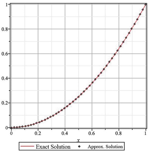
Table 1. Numerical results for Example, 3.1

$x$	Exact value $y(x)$	Approx. value $y(x)$	Absolute errors
$0.10$	$1.105170918$	$1.105170918$	$0$
$0.18$	$1.197217363$	$1.197217364$	$1.0\times {10}^{-9}$
$0.25$	$1.284025417$	$1.284025416$	$1.0\times {10}^{-9}$
$0.37$	$1.447734615$	$1.447734613$	$2.0\times {10}^{-9}$
$0.50$	$1.648721271$	$1.648721269$	$2.0\times {10}^{-9}$
$0.78$	$2.181472265$	$2.181472192$	$7.3\times {10}^{-8}$
$1.00$	$2.718281828$	$2.718281267$	$5.61\times {10}^{-7}$

In Figure 3, we show the graphical comparison between the exact solution and the approximate solution obtained by the proposed method at the level $n=5$ and the absolute errors $E_4,E_5$, and $E_6$ are given in Table 2.

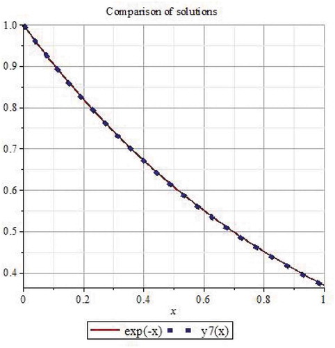
Example 3.4. Consider a following NFDE with proportional delay (Biazar & Ghanbari, 2012)

$y^{\prime }(x)=\frac{1}{2}y\left(\frac{x}{2}\right)-y(x)+\frac{1}{2}{y}^{\prime }\left(\frac{x}{2}\right)x\in [0,1]$

$y(0)=1.$

Table 2. Numerical results for Example, 3.3

$x$	$E_4$	$E_5$	$E_6$
$0.20$	$4.09e-7$	$5.12e-8$	$6.40e-10$
$0.40$	$6.90e-6$	$8.63e-7$	$1.07e-7$
$0.60$	$3.69e-5$	$4.62e-6$	$5.78e-7$
$0.80$	$1.24e-4$	$1.55e-5$	$1.94e-6$
$1.00$	$3.25e-4$	$4.07e-5$	$5.09e-6$

Following the proposed method, similar to Example 3.1, the seventh order of HPM approximate solution is

$y_7(x)=1-\frac{127}{128}x+\frac{8001}{16384}{x}^2-\frac{82677}{524288}{x}^3+\frac{1240155}{33554432}{x}^4-\frac{1736217}{268435456}{x}^5$

$+\frac{1736217}{2147483648}{x}^6-\frac{248031}{4294967296}{x}^7,$

and the exact solution of the given NFDE is $y(x)=e^{-x}$. The graphical comparison of the approximate solution at seventh iteration with the exact solution is shown in Figure 4. From Figure 4, it is clear that the approximate solution almost same as the exact solution.

Figure 4. Comparison of approximate and Exact solutions for Example 3.4.

4. Conclusion

In this article, we presented a new symbolic method for solving the neutral functional-differential equations with variable coefficients via homotopy perturbation method to obtain quick and accurate solution. We also presented several examples and comparisons of the results obtained by the proposed method with the exact solution reveals that the present method is very effective and convenient. This theory can also be easily extended to fractal calculus, i.e., one can try to apply the proposed method to get the approximate solution for fractal calculus problems.

Acknowledgements

The authors sincerely thank to the anonymous reviewers and editor for their valuable suggestions and remarkable comments to improve the content of this manuscript.

Additional information

Funding

The authors received no direct funding for this research.

Notes on contributors

Srinivasarao Thota

Srinivasarao Thota (corresponding author) completed his M.Sc. in Mathematics from Indian Institute of Technology (IIT) Madras, India and Ph.D. in Mathematics from Motilal Nehru National institute of Technology (NIT) Allahabad, India. His research interests are Computer Algebra (Symbolic methods for differential equations), Numerical Analysis (Root finding algorithms) and Mathematical Modelling (Ecology). He has published more than 30 research papers in various international journals and attended and presented research work in several national and international conferences. Also, he had given more than 9 special/invited conferences talks. He has more than 10 years of teaching and research experience. Presently, he is working at Department of Applied Mathematics, School of Applied Natural Sciences, Adama Science and Technology University, Ethiopia.

References

- Biazar, J., & Ghanbari, B. (2012). The homotopy perturbation method for solving neutral functional-differential equations with proportional delays. Journal of King Saud University-Science, 24(1), 33–13. https://doi.org/10.1016/j.jksus.2010.07.026
- Biazar, J., & Ghazvini, H. (2008). Homotopy perturbation method for solving hyperbolic partial differential equations. Computers & Mathematics with Applications, 56(2), 453–458. https://doi.org/10.1016/j.camwa.2007.10.032
- Chen, X., & Wang, L. (2010). The variational iteration method for solving a neutral functional-differential equation with proportional delays. Computer and Mathematics with Applications, 59(8), 2696–2702. https://doi.org/10.1016/j.camwa.2010.01.037
- Coddington, E. A., & Levinson, N. (1955). Theory of ordinary differential equations. McGraw-Hill Book Company, Inc.
- Collins, P. J. (2006). Differential and integral equations. Oxford University Press.
- Derfel, G. A., & Vogl, F. (1996). On the asymptotics of solutions of a class of linear functional-differential equations. European Journal of Applied Mathematics, 7(5), 511–518. https://doi.org/10.1017/S0956792500002527
- Feldstein, A., & Liu, Y. (1998). On neutral functional-differential equations with variable time delays, Math. Mathematical Proceedings of the Cambridge Philosophical Society, 124(2), 371–384. https://doi.org/10.1017/S0305004198002497
- He, J. H. (1999). Homotopy perturbation technique. Computer Methods in Applied Mechanics and Engineering, 178(3–4), 257–262. https://doi.org/10.1016/S0045-7825(99)00018-3
- He, J. H. (2000). A coupling method of homotopy technique and a perturbation technique for non linear problems. International Journal of Non-Linear Mechanics, 35(1), 37–43. https://doi.org/10.1016/S0020-7462(98)00085-7
- He, J. H. (2004). The homotopy perturbation method for nonlinear oscillators with discontinuities. Applied Mathematics and Computation, 151, 287–292.
- He, J. H. (2019). The simpler, the better: Analytical methods for nonlinear oscillators and fractional oscillators. Journal of Low Frequency Noise, Vibration and Active Control, 38(3–4), 1252–1260. https://doi.org/10.1177/1461348419844145
- He, J. H., & Ain, Q. T. (2020). New promises and future challenges of fractal calculus: From two-scale Thermodynamics to fractal variational principle. Thermal Science, 24(2A), 659–681. https://doi.org/10.2298/TSCI200127065H
- He, J. H., & Jin, X. (2020). A short review on analytical methods for the capillary oscillator in a nanoscale deformable tube. Mathematical Methods in the Applied Sciences, 1-8. http://dx.doi.org/10.1002/mma.6321
- Jafari, M. A., & Aminataei, A. (2012). Method of successive approximations for solving the multi-pantograph delay equations. General Mathematics Notes, 8(1), 23–28. https://www.emis.de/journals/GMN/yahoo_site_admin/assets/docs/4_GMN-892-V8N1.160183624.pdf
- Sezer, M., Yalcinbas, S., & Sahin, N. (2008). Approximate solution of multi-pantograph equation with variable coefficients. Journal of Computational and Applied Mathematics, 241(2), 406–416. https://doi.org/10.1016/j.cam.2007.03.024
- Shakeri, F., & Dehghan:, M. (2008). Solution of delay differential equations via a homotopy perturbation method. Mathematical and Computer Modelling, 48(3–4), 486–498. https://doi.org/10.1016/j.mcm.2007.09.016
- Shang:, Y. (2012). A lie algebra approach to susceptible-infected-susceptible epidemics. Electronic Journal of Differential Equations, 2012(233), 1–7. https://ejde.math.txstate.edu/Volumes/2012/233/abstr.html
- Thota, S. A study on symbolic algorithms for solving ordinary and partial linear differential equations, Ph.D. thesis, Motilal Nehru national Institute of Technology Allahabad. (2017).
- Thota, S. (2018a). On a new symbolic method for initial value problems for systems of higher-order linear differential equations. International Journal of Mathematical Models and Methods in Applied Sciences, 12, 194–202. https://www.naun.org/main/NAUN/ijmmas/2018/a502001-adw.pdf
- Thota, S. (2018b). A symbolic algorithm for polynomial interpolation with integral conditions. Applied Mathematics & Information Sciences, 12(5), 995–1000. https://doi.org/10.18576/amis/120512
- Thota, S. (2018c). Initial value problems for system of differential-algebraic equations in Maple. BMC Research Notes, 11(1), 651. https://doi.org/10.1186/s13104-018-3748-0
- Thota, S. (2018d). On a symbolic method for error estimation of a mixed interpolation. Kyungpook Mathematical Journal, 58(3), 453–462. https://doi.org/10.5666/KMJ.2019.59.1.13
- Thota, S. (2019). On a new symbolic method for solving two-point boundary value problems with variable coefficients. International Journal of Mathematics and Computers in Simulation, 13, 160–164. https://www.naun.org/main/NAUN/mcs/2019/a502002-abh.pdf
- Thota, S. (2019a). On a symbolic method for fully inhomogeneous boundary value problems. Kyungpook Mathematical Journal, 59(1), 13–22.
- Thota, S. (2019b). A symbolic algorithm for polynomial interpolation with stieltjes conditions in maple. Proceedings of the Institute of Applied Mathematics, 8(2), 112–120.
- Thota, S., & Kumar, S. D. (2015). A new method for general solution of system of higher-order linear differential equations. International Conference on Inter Disciplinary Research in Engineering and Technology, 1, 240–243. https://edlib.net/2015/icidret/icidret2015039.html
- Thota, S., & Kumar, S. D. Symbolic method for polynomial interpolation with Stieltjes conditions, International conference on frontiers in mathematics (2015), Gauhati University, Guwahati, Assam, India. 225–228.
- Thota, S., & Kumar, S. D. (2016). Solving system of higher-order linear differential equations on the level of operators. International Journal of Pure and Apllied Mathematics, 106(4), 11–21. https://doi.org/10.12732/ijpam.v106i4.1
- Thota, S., & Kumar, S. D. (2016a). On a mixed interpolation with integral conditions at arbitrary nodes. Cogent Mathematics, 3(1), 1–10. https://doi.org/10.1080/23311835.2016.1151613
- Thota, S., & Kumar, S. D. (2016b). Symbolic algorithm for a system of differential-algebraic equations. Kyungpook Mathematical Journal, 56(4), 1141–1160. https://doi.org/10.5666/KMJ.2016.56.4.1141
- Thota, S., & Kumar, S. D. (2017). Maple implementation of symbolic methods for initial value problems. Research for Resurgence-An Edited Multidisciplinary Research Book, I(1), 240–243. https://d1wqtxts1xzle7.cloudfront.net/55878169/Chapter_3_SThota.pdf?1519376397=&response-content-disposition=inline%3B+filename%3DMaple_Implementation_of_Symbolic_Methods.pdf&Expires=1599120501&Signature=BvC-eJGrqP~tBOjPZfZC5thyXxUgJrj-X2lPR5ZP0RMEKprV1FdZ~mpjTYqyi0PwuFe9bIvoZtWq~8FyShZko4QQuOwRIYlvUhDotPxmm59v1RkoFpeUYhwiGAR9C~RKPxJuHBsvkY21s-4nAGM5LqqWuvlpK8hu86LxFcuQtVZuKI5i96Qgika6OcnOeR3SXhGr2by8K8Al2VCTcw7ZRMLqD7Fz7mOZVwneh8OaFU6dSU5KYBBuT1~8e1G3lstPEni6CIAeFaG7p~52W4ceoG2ZlLLR7CiASZXkYYsCQ2KyuBrVysd-qvR2FsHGX~VAw2n7le~HSKFn84Bc85tnlA__&Key-Pair-Id=APKAJLOHF5GGSLRBV4ZA
- Thota, S., Rosenkranz, M., & Kumar, S. D. Solving systems of linear differential equations over integro-differential algebras, International conference on applications of computer algebra, June 24–29, 2012, Sofia, Bulgaria.