Computational method for singularly perturbed two-parameter parabolic convection-diffusion problems

Abstract

This paper deals with the numerical solution of singularly perturbed parabolic convection-diffusion problems with two small positive parameters multiplying the convection and diffusion terms. A parameter-uniform computational method is developed to solve these problems. The stability and consistency of the method are well established. Numerical experimentation is done and it is observed that the formulated method is stable, consistent and gives more accurate results than some methods exist in the literature.

Keywords:

• singularly perturbed
• parabolic convection-diffusion
• computational method
• two-parameter
• parameter uniform

PUBLIC INTEREST STATEMENT

Singularly perturbed differential equations are very important to describe some phenomena like viscous flow of fluids at high Reynolds number, convective heat transport problem, electromagnetic field problem in moving media, financial modeling, and turbulence model, reaction-diffusion process, etc. The solution to such problems changes unexpectedly in some regions of the domain where it exhibits boundary layers. The construction of numerical schemes which is not affected by the singular perturbation parameter is, however, not an easy task because of the singularity in the layer regions. But, the present work formulated a numerical method that is convergent independent of the effect of the singular perturbation parameter and is very helpful for scholars working in the aforementioned areas.

1. Introduction

Singularly perturbed problems (SPPs) play a significant role in applied sciences and engineering like quantum mechanics, modelling of water quality problems in river networks, fluid flow at high Reynolds/Peclet numbers, drift-diffusion equation of semiconductor device modeling, control theory like control of aerospace, chemical flow reactor theory, lubrication theory, etc. These and other applications are given in Kadalbajoo and Yadaw (2012), Patidar (2008), Phaneendra and Mahesh (2017), Ramos (2005), Zahra et al. (2014), and Zahra and El Mhlawy (2013) the references therein. So finding the solutions to such problems is an important phenomenon and essential in these applications.

The main characteristics of such problems are the swift growth or deterioration of their solutions in one or more narrow boundary layer region(s). In most cases, not only determining analytical solutions to such problems is difficult but also the convergence analysis due to the presence of boundary layers and multi-scale characters in their solution. As a result, the classical finite difference method is not reliable to preserve the stability property as they require the introduction of very fine meshes inside the boundary layers, which requires more computational cost. Even in contrary to the usual expectation, the maximum point-wise error may not decrease as the mesh is refined. To get rid of such shortcomings, we need to develop simple and more accurate computational methods that also convergent independent of the value of the perturbation parameter for solving the problem under consideration.

In comparison to problems with one parameter (singularly perturbed problems), only a few researchers tackled problems with two parameters. Although O’Malley was the kick starter to study the asymptotic solution of problems with two parameters in the mid-1960s, much is not known about robust numerical methods for solving these problems until the authors Vulanović (2001), O’Riordan et al. (2003), and Roos and Uzelac (2003) published their work.

So far, some fitted numerical methods with different approaches have been developed. In the formulation of the methods, it is mandatory either to have a priori information about the behaviour of derivatives of the exact solution for refining the mesh or simply try to use an adaptive method. To mention some: Chandru et al. (2019), Clavero et al. (2017), Gupta et al. (2019), Jha and Kadalbajoo (2015), Kadalbajoo and Yadaw (2012), Khandelwal and Khan (2017), O’Riordan et al. (2006), Phaneendra and Mahesh (2017), Zahra et al. (2014), and Zahra and El Mhlawy (2013) proposed a numerical scheme depending on a priori information for the problem under consideration using piecewise uniform mesh. Bullo et al. (2019), Kadalbajoo and Jha (2012), Munyakazi (2015), and Patidar (2008) constructed a numerical scheme using uniform mesh. For a priori information about the solution is not known, Das and Mehrmann (2016) constructed an adaptive mesh method that automatically detects the layer region.

Further, the heat transfer problem of laminar fluid flow, commonly called the Graetz problem, is solved analytically through the separation of variable by Belhocine and Wan Omar (2017) and numerically based on orthogonal collocation, followed by the Crank-Nicholson finite difference method by Belhocine (2016) and Belhocine (2017). On the other hand, a nonlinear Partial Differential Equation (PDE) with fractional order time derivative that better express nonlinear diffusion phenomena than integer order has been treated by the fractional symmetry group method Liu et al. (2019) and symmetry analysis method Liu et al. (2020). These methods constitute reducing the problem into a fractional ordinary differential equation (ODE) based on the symmetry obtained.

Most of the aforementioned schemes developed for the problem with one perturbation parameter where it is multiplied with its highest order derivative. Here, our concern is with a problem involving two perturbation parameters that affect the second- and first-order derivative terms. To develop the methods, Clavero et al. (2017), Chandru et al. (2019), Das and Mehrmann (2016), Gupta et al. (2019), Jha and Kadalbajoo (2015), Munyakazi (2015), and Zahra et al. (2014) used the classical Euler method for temporal discretization. Clavero et al. (2017) and Chandru et al. (2019) considered if there is a discontinuity in the data. The former authors used a simple upwind finite difference scheme on a Shishkin mesh for the spatial discretization. But, the latter authors used upwind and backward finite difference approximation in different sections of the domain.

In this paper, we treated the time-dependent two-parameter singularly perturbed initial-boundary value problem (IBVP) (1)-(3), using uniform meshes in a different approach from that of Munyakazi (2015) and Bullo et al. (2019). We have designed a numerical scheme based on two steps; semi-temporal discretization followed by spatial discretization. First, we have used the Crank-Nicholson method to discretize the time variable, and then the central difference approximation on the nonstandard methodology of Mickens for the space variable. A denominator function has been introduced in the nonstandard method, in such a way that it suits the central difference. The stability analysis of the method is treated by the von Neumann stability analysis technique.

2. Problem formulation

Consider a cluster of a one-dimensional parabolic time-dependent convection-diffusion problem with two perturbation parameters multiplying the convection and diffusion terms given by Das and Mehrmann (2016). So we need to find an approximate solution to a function $u(x,t)$ in the domain $D=\mathrm{\Omega }\times (0,T],\mathrm{\Omega }=(0,1)$ which satisfies

(1) $L_{\epsilon ,\mu }u:=\frac{\mathrm{\partial }u}{\mathrm{\partial }t}-\epsilon \frac{{\mathrm{\partial }}^{2}u}{\mathrm{\partial }{x}^2}-\mu a(x,t)\frac{\mathrm{\partial }u}{\mathrm{\partial }x}+b(x,t)u=f(x,t),(x,t)\in D,$(1)

together with initial and boundary conditions

(2) $u(x,0)=u_0(x),x\in \bar{\mathrm{\Omega }},$(2)

(3) $u(0,t)=0=u(1,t),t\in [0,T].$(3)

where $0<\epsilon \ll 1$ and $0<\mu \ll 1$ are two perturbation parameters, and we suppose that the coefficient $a(x,t)$ of the convection term, $b(x,t)$ of the reaction term, and the source term $f(x,t)$ are sufficiently smooth such that $a(x,t)\ge \alpha >0,b(x,t)\ge \beta >0$ for all $(x,t)\in D$. We also assume that sufficient smoothness and suitability of the function $u_0(x)$ at the two endpoints $(0,0)$ and $(1,0)$ (i.e. $u_0(0)=0=u_0(1)$), to be guaranteed of the existence and uniqueness of the solution $u(x,t)$.

The rest of this paper is organized as follows. In section 3, the detailed description of the method is given. The stability and convergence analysis of the current method is given in section 4. In section 5, the behavior of the scheme is verified by numerical examples. Discussion of the results and conclusion of our work are provided in section 6.

3. Formulation of the numerical scheme

This section deals with the detailed description of the method and its analysis.

Time variable discretization: Let $k$ be the step size in the time direction and $M$ be the number of subintervals of $[0,T]$ with equal length. This gives a time mesh

$D_t^M=\left\{t_m=(m-1)k,m=1,2,\dots ,M+1,k=\frac{T}{M}\right\}.$

Using the Crank-Nicholson method, we obtain

$\frac{u(x,t_m)-u(x,t_{m-1})}{k}-\epsilon \frac{u_{xx}(x,t_m)+u_{xx}(x,t_{m-1})}{2}+$

$\mu \frac{a(x,t_m)u_x(x,t_m)+a(x,t_{m-1})u_x(x,t_{m-1})}{2}-$

$\frac{b(x,t_m)u(x,t_m)+b(x,t_{m-1})u(x,t_{m-1})}{2}=\frac{f(x,t_m)+f(x,t_{m-1})}{2}.$

subject to the condition

$u(x,0)=u_0(x),\mathrm{\forall }x\in \mathrm{\Omega }\mathrm{a}\mathrm{n}\mathrm{d}u(0,t_m)=0,u(1,t_m)=0,m=1,2,\dots ,M+1,$

which is a system of linear equations in space at each time. Now collecting the $(m)$th and $(m-1)$th time level, we obtain

$\frac{u(x,t_m)}{k}-\frac{\epsilon }{2}{u}_{xx}(x,t_m)-\frac{\mu a(x,t_m)}{2}{u}_x(x,t_m)+\frac{b(x,t_m)}{2}u(x,t_m)=\frac{u(x,t_{m-1})}{k}$

$+\frac{\epsilon }{2}{u}_{xx}(x,t_{m-1})+\frac{\mu a(x,t_{m-1})}{2}{u}_x(x,t_{m-1})-\frac{b(x,t_{m-1})}{2}u(x,t_{m-1})$

(4) $+\frac{f(x,t_m)+f(x,t_{m-1})}{2}.$(4)

Rearranging we can write it as

$-\epsilon u_{xx}(x,t_m)-\mu a(x,t_m)u_x(x,t_m)+\left(b(x,t_m)+\frac{2}{k}\right)u(x,t_m)=\epsilon u_{xx}(x,t_{m-1})+$

$\mu a(x,t_{m-1})u_x(x,t_{m-1})-\left(b(x,t_{m-1})-\frac{2}{k}\right)u(x,t_{m-1})+f(x,t_m)+f(x,t_{m-1}).$

(5) ${\bar{L}}_{\epsilon ,\mu }u(x,t_m):\equiv -\epsilon u_{xx}(x,t_m)-\mu a(x,t_m)u_x(x,t_m)+q(x,t_m)u(x,t_m)=g(x,t_m),$(5)

where

$q(x,t_m)=\left(b(x,t_m)+\frac{2}{k}\right),$

$g(x,t_m)=\epsilon u_{xx}(x,t_{m-1})+\mu a(x,t_{m-1})u_x(x,t_{m-1})-\left(b(x,t_{m-1})-\frac{2}{k}\right)u(x,t_{m-1})$

(6) $+f(x,t_m)+f(x,t_{m-1}).$(6)

Truncation Error: The error estimate in the temporal direction is obtained using Taylor’s theorem. Now, we can express

(7) $u(x,t_m)=u(x,t_{m-1/2+1/2})=u(x,t_{m-1/2}+k/2),$(7)

and

(8) $u(x,t_{m-1})=u(x,t_{m-1/2-1/2})=u(x,t_{m-1/2}-k/2).$(8)

Then, Equation (4)(4) $+\frac{f(x,t_m)+f(x,t_{m-1})}{2}.$(4) becomes

$\frac{u(x,t_m)-u(x,t_{m-1})}{k}=\epsilon \frac{u_{xx}(x,t_m)+u_{xx}(x,t_{m-1})}{2}$

$+\mu \frac{a(x,t_m)u_x(x,t_m)+a(x,t_{m-1})u_x(x,t_{m-1})}{2}$

(9) $-\frac{b(x,t_m)u(x,t_m)+b(x,t_{m-1})u(x,t_{m-1})}{2}+\frac{f(x,t_m)+f(x,t_{m-1})}{2}.$(9)

From Taylor’s series expansion about the point $(x,t_{m-1/2})$, we have

$u(x,t_m)=u(x,t_{m-1/2})+\frac{(k/2)}{1!}\frac{\mathrm{\partial }u}{\mathrm{\partial }t}(x,t_{m-1/2})+\frac{{(k/2)}^2}{2!}\frac{{\mathrm{\partial }}^{2}u}{\mathrm{\partial }{t}^2}(x,t_{m-1/2})$

(10) $+\frac{{(k/2)}^3}{3!}\frac{{\mathrm{\partial }}^{3}u}{\mathrm{\partial }{t}^3}(x,t_{m-1/2})+\dots ,$(10)

$u(x,t_{m-1})=u(x,t_{m-1/2})-\frac{(k/2)}{1!}\frac{\mathrm{\partial }u}{\mathrm{\partial }t}(x,t_{m-1/2})+\frac{{(k/2)}^2}{2!}\frac{{\mathrm{\partial }}^{2}u}{\mathrm{\partial }{t}^2}(x,t_{m-1/2})$

(11) $-\frac{{(k/2)}^3}{3!}\frac{{\mathrm{\partial }}^{3}u}{\mathrm{\partial }{t}^3}(x,t_{m-1/2})+\dots$(11)

Subtracting Equation (11)(11) $-\frac{{(k/2)}^3}{3!}\frac{{\mathrm{\partial }}^{3}u}{\mathrm{\partial }{t}^3}(x,t_{m-1/2})+\dots$(11) from Equation (10)(10) $+\frac{{(k/2)}^3}{3!}\frac{{\mathrm{\partial }}^{3}u}{\mathrm{\partial }{t}^3}(x,t_{m-1/2})+\dots ,$(10) gives

(12) $\frac{\mathrm{\partial }u}{\mathrm{\partial }t}(x,t_{m-1/2})=\frac{u(x,t_m)-u(x,t_{m-1})}{k}+{\tau }_1,$(12)

where

${\tau }_1=-\frac{k^2}{24}\frac{{\mathrm{\partial }}^{3}u}{\mathrm{\partial }{t}^3}(x,t_{m-1/2})\equiv O(k^2).$

This indicates that the error estimate of the time discretization is

(13) $\parallel T{E}_1\parallel \le C(k^2),$(13)

where $C={max}_{x,t\in [0,1]}\left|-\frac{{\mathrm{\partial }}^{3}u}{\mathrm{\partial }{t}^3}(x,t)\right|$ is a positive constant independent of the perturbation parameters $\epsilon$ and $\mu$ and the time mesh size $k$.

Spatial variable discretization: Let $h$ be the step size in spatial direction and $N$ be the number of subintervals of $[0,1]$ with equal length. This gives a space mesh

$D_x^N=\left\{x_n=(n-1)h,n=1,2,\dots ,N+1,h=\frac{1}{N}\right\}.$

Now fixing the time variable, and considering the homogeneous part of Equation (5)(5) ${\bar{L}}_{\epsilon ,\mu }u(x,t_m):\equiv -\epsilon u_{xx}(x,t_m)-\mu a(x,t_m)u_x(x,t_m)+q(x,t_m)u(x,t_m)=g(x,t_m),$(5) with constant coefficients, where the constant coefficients are the lower bounds of the coefficient functions, we get

$-\epsilon \frac{d^{2}u}{d{x}^2}-\mu \alpha \frac{du}{dx}+q^{\ast }u=0,$

where $q(x,t_m)\ge q^{\ast }>0$. Its characteristic equation is $-\epsilon r^2(x)-\mu \alpha r(x)+q^{\ast }=0$. This has two independent solutions (say):

$r_1=\frac{\mu \alpha +\sqrt{{\mu }^2{\alpha }^2+4\epsilon q^{\ast }}}{-2\epsilon }\mathrm{a}\mathrm{n}\mathrm{d}{r}_2=\frac{\mu \alpha -\sqrt{{\mu }^2{\alpha }^2+4\epsilon q^{\ast }}}{-2\epsilon },$

that describes the boundary layers at $x=0$ and $x=1$ respectively. This is shown by Munyakazi (2015) and Bullo et al. (2019) in two cases ${\mu }^2\le C\epsilon$ and ${\mu }^2\ge C\epsilon$. Let the approximate solution to $u(x,t_m)$ at the grid point $x_n$ be given by

$U_n=Aexp(r_1{x}_n)+Bexp(r_2{x}_n).$

Using the construction of nonstandard finite difference (NSFD) methodology of Mickens (2000) and Mickens (2005), we have the determinant

(14) $\left|\begin{array}{ccc}{U}_{n-1}& exp(r_1{x}_{n-1})& exp(r_2{x}_{n-1})\\ U_n& exp(r_1{x}_n)& exp(r_2{x}_n)\\ U_{n+1}& exp(r_1{x}_{n+1})& exp(r_2{x}_{n+1})\end{array}\right|=0.$(14)

$\left|\begin{array}{ccc}{U}_{n-1}& exp(r_1{x}_n-r_{1}h)& exp(r_2{x}_n-r_{2}h)\\ U_n& exp(r_1{x}_n)& exp(r_2{x}_n)\\ U_{n+1}& exp(r_1{x}_n+r_{1}h)& exp(r_2{x}_n+r_{2}h)\end{array}\right|=0,$

$exp(r_1{x}_n+r_2{x}_n)\left|\begin{array}{ccc}{U}_{n-1}& exp(-r_{1}h)& exp(-r_{2}h)\\ U_n& 1& 1\\ U_{n+1}& exp(r_{1}h)& exp(r_{2}h)\end{array}\right|=0.$

Evaluation of the determinant and simplification of the terms using double angle formula for hyperbolic functions yields

(15) $exp\left(\frac{-\mu \alpha h}{2\epsilon }\right)U_{n-1}-2cosh\left(\frac{h\sqrt{{\mu }^2{\alpha }^2+4\epsilon q^{\ast }}}{2\epsilon }\right)U_n+exp\left(\frac{\mu \alpha h}{2\epsilon }\right)U_{n+1}=0.$(15)

According to Mickens (2000), the scheme given in Equation (15)(15) $exp\left(\frac{-\mu \alpha h}{2\epsilon }\right)U_{n-1}-2cosh\left(\frac{h\sqrt{{\mu }^2{\alpha }^2+4\epsilon q^{\ast }}}{2\epsilon }\right)U_n+exp\left(\frac{\mu \alpha h}{2\epsilon }\right)U_{n+1}=0.$(15) is said to be ’exact’ in the sense that it has the same general solution as the corresponding differential equation. To construct the nonstandard finite difference scheme, we need to find a suitable denominator function which replaces $h^2$. But, it is not as such a simple thing to do directly from Equation (15)(15) $exp\left(\frac{-\mu \alpha h}{2\epsilon }\right)U_{n-1}-2cosh\left(\frac{h\sqrt{{\mu }^2{\alpha }^2+4\epsilon q^{\ast }}}{2\epsilon }\right)U_n+exp\left(\frac{\mu \alpha h}{2\epsilon }\right)U_{n+1}=0.$(15) . Patidar (2008) emphasized the fact that the layer behaviors of the solution of Equation (5)(5) ${\bar{L}}_{\epsilon ,\mu }u(x,t_m):\equiv -\epsilon u_{xx}(x,t_m)-\mu a(x,t_m)u_x(x,t_m)+q(x,t_m)u(x,t_m)=g(x,t_m),$(5) and that of the problem in the case when $q^{\ast }=0$ are similar (Gupta et al., 2019). So, considering the exact scheme for the latter case, we get

$exp\left(\frac{-\mu \alpha h}{2\epsilon }\right)U_{n-1}-\left(exp\left(\frac{\mu \alpha h}{2\epsilon }\right)+exp\left(\frac{-\mu \alpha h}{2\epsilon }\right)\right)U_n+exp\left(\frac{\mu \alpha h}{2\epsilon }\right)U_{n+1}=0.$

Now, multiplying both sides by 2, and then adding and subtracting the terms $exp\left(\frac{\mu \alpha h}{2\epsilon }\right)U_{n-1}$ and $exp\left(\frac{-\mu \alpha h}{2\epsilon }\right)U_{n+1}$, yields

$\left(exp\left(\frac{\mu \alpha h}{2\epsilon }\right)+exp\left(\frac{-\mu \alpha h}{2\epsilon }\right)\right)\left(U_{n+1}-2Un+U_{n-1}\right)$

$+\left(exp\left(\frac{\mu \alpha h}{2\epsilon }\right)-exp\left(\frac{-\mu \alpha h}{2\epsilon }\right)\right)\left(U_{n+1}-U_{n-1}\right)=0.$

This can definitely be written as

(16) $-\epsilon \frac{U_{n-1}-2U_n+U_{n+1}}{\frac{2h\epsilon }{-\mu \alpha }tanh\left(\frac{-\mu \alpha h}{2\epsilon }\right)}-\mu \alpha \frac{U_{n+1}-U_{n-1}}{2h}=0.$(16)

As we can observe, the classical denominator $h^2$ is replaced by the denominator function ${\gamma }^2=\frac{2h\epsilon }{-\mu \alpha }tanh\left(\frac{-\mu \alpha h}{2\epsilon }\right)$ (due to which the method is called nonstandard), and implementing it for the variable coefficient problem at $(m)$th time level we get

(17) ${\gamma }_{n,m}^2=\frac{2h\epsilon }{-\mu a_n^m}tanh\left(\frac{-\mu a_n^{m}h}{2\epsilon }\right),$(17)

where $a_n^m=a(x_n,t_m)$.

Remark 1.1: From the power series expansion of hyperbolic tangent function we have

${\gamma }^2=\frac{2h\epsilon }{-\mu \alpha }tanh\left(\frac{-\mu \alpha h}{2\epsilon }\right)$

$=\frac{2h\epsilon }{-\mu \alpha }\left[\frac{-\mu \alpha h}{2\epsilon }-\frac{1}{3}{\left(\frac{-\mu \alpha h}{2\epsilon }\right)}^3+\frac{2}{15}{\left(\frac{-\mu \alpha h}{2\epsilon }\right)}^5+\dots \right],$

${\gamma }^2\approx h^2-\frac{h^4}{12}\frac{{\mu }^2{\alpha }^2}{{\epsilon }^2}.$

The total discrete scheme is obtained by using Equation (17)(17) ${\gamma }_{n,m}^2=\frac{2h\epsilon }{-\mu a_n^m}tanh\left(\frac{-\mu a_n^{m}h}{2\epsilon }\right),$(17) into Equation (4)(4) $+\frac{f(x,t_m)+f(x,t_{m-1})}{2}.$(4) as

$\frac{U_n^m}{k}-\frac{\epsilon }{2}\left(\frac{U_{n-1}^m-2U_n^m+U_{n+1}^m}{{\gamma }_{n,m}^2}\right)-\frac{\mu a_n^m}{2}\left(\frac{U_{n+1}^m-U_{n-1}^m}{2h}\right)+\frac{b_n^m}{2}{U}_n^m$

$=\frac{U_n^{m-1}}{k}+\frac{\epsilon }{2}\left(\frac{U_{n-1}^{m-1}-2U_n^{m-1}+U_{n+1}^{m-1}}{h^2}\right)+\frac{\mu a_n^{m-1}}{2}\left(\frac{U_{n+1}^{m-1}-U_{n-1}^{m-1}}{2h}\right)$

$-\frac{b_n^{m-1}}{2}{U}_n^{m-1}+\frac{1}{2}\left(f_n^m+f_n^{m-1}\right).$

It can be written as

$U_n^m+k\left[A_n^{-}{U}_{n-1}^m+A_n^c{U}_n^m+A_n^{+}{U}_{n+1}^m\right]=U_n^{m-1}$

$+k\left[B_n^{-}{U}_{n-1}^{m-1}+B_n^c{U}_n^{m-1}+B_n^{+}{U}_{n+1}^{m-1}\right]+F_n^m,$

(18) $\mathrm{f}\mathrm{o}\mathrm{r}n=2,3,\dots ,N,m=2,3,\dots ,M+1,$(18)

subject to the conditions

$U_n^1=u_0(x_n),n=1,2,3,\dots ,N,U_1^m=0=U_{N+1}^m,m=1,2,3,\dots ,M+1,$

where

$A_n^{-}=-\frac{\epsilon }{2{\gamma }_{n,m}^2}+\frac{\mu a_n^m}{4h},B_n^{-}=\frac{\epsilon }{2h^2}-\frac{\mu a_n^{m-1}}{4h},$

$A_n^c=\frac{\epsilon }{{\gamma }_{n,m}^2}+\frac{b_n^m}{2},B_n^c=-\frac{\epsilon }{h^2}-\frac{b_n^{m-1}}{2},$

$A_n^{+}=-\frac{\epsilon }{2{\gamma }_{n,m}^2}-\frac{\mu a_n^m}{4h},B_n^{+}=\frac{\epsilon }{2h^2}+\frac{\mu a_n^{m-1}}{4h},$

$F_n^m=\frac{k}{2}\left(f_n^m+f_n^{m-1}\right).$

In our case, the given boundary conditions are zero (we can insert linear combinations in the first and last equations as follows). Associating this fact together with Equation (18)(18) $\mathrm{f}\mathrm{o}\mathrm{r}n=2,3,\dots ,N,m=2,3,\dots ,M+1,$(18) , we can obtain a linear $(N+1)\times (N+1)$ system of equations at $m$th time level as

$U_1^m+k{U}_1^m=U_1^{m-1}+k{U}_1^{m-1}+0,$

$U_2^m+k[A_2^{-}{U}_1^m+A_2^c{U}_2^m+A_2^{+}{U}_3^m]=U_2^{m-1}+k[B_2^{-}{U}_1^{m-1}+B_2^c{U}_2^{m-1}+B_2^{+}{U}_3^{m-1}]+F_2^m,$

$U_3^m+k[A_3^{-}{U}_2^m+A_3^c{U}_3^m+A_3^{+}{U}_4^m]=U_3^{m-1}+k[B_3^{-}{U}_2^{m-1}+B_3^c{U}_3^{m-1}+B_3^{+}{U}_4^{m-1}]+F_3^m,$

$U_4^m+k[A_4^{-}{U}_3^m+A_4^c{U}_4^m+A_4^{+}{U}_5^m]=U_4^{m-1}+k[B_4^{-}{U}_3^{m-1}+B_4^c{U}_4^{m-1}+B_4^{+}{U}_5^{m-1}]+F_4^m,$

$\dots \dots \dots ,$

$U_N^m+k[A_N^{-}{U}_{N-1}^m+A_N^c{U}_N^m+A_N^{+}{U}_{N+1}^m]=U_N^{m-1}+k[B_N^{-}{U}_{N-1}^{m-1}+B_N^c{U}_N^{m-1}+B_N^{+}{U}_{N+1}^{m-1}]+F_N^m,$

$U_{N+1}^m+k{U}_{N+1}^m=U_{N+1}^{m-1}+k{U}_{N+1}^{m-1}+0.$

This yields a matrix form

(19) $\left(I+kA\right)V^m=\left(I+kB\right)V^{m-1}+H^m,m=2,\dots ,M+1.$(19)

The solution of Equation (19)(19) $\left(I+kA\right)V^m=\left(I+kB\right)V^{m-1}+H^m,m=2,\dots ,M+1.$(19) can be obtained by the matrix inversion method, where

$I=\left(\begin{array}{ccccc}1& 0& 0& \dots & 0\\ 0& 1& 0& \dots & 0\\ 0& 0& 1& \dots & 0\\ \dots & \dots & \dots & \dots & \dots \\ 0& 0& 0& \dots & 1\end{array}\right),A=\left(\begin{array}{cccccc}1& 0& 0& 0& \dots & 0\\ A_2^{-}& A_2^{-c}& A_2^{+}& 0& \dots & 0\\ 0& A_3^{-}& A_3^c& A_3^{+}& \dots & 0\\ \dots & \dots & \dots & \dots & \dots & \dots \\ 0& \dots & 0& A_N^{-}& A_N^c& A_N^{+}\\ 0& 0& 0& \dots & 0& 1\end{array}\right),$

$B=\left(\begin{array}{cccccc}1& 0& 0& 0& \dots & 0\\ B_2^{-}& B_2^{-c}& B_2^{+}& 0& \dots & 0\\ 0& B_3^{-}& B_3^c& B_3^{+}& \dots & 0\\ \dots & \dots & \dots & \dots & \dots & \dots \\ 0& \dots & 0& B_N^{-}& B_N^c& B_N^{+}\\ 0& 0& 0& \dots & 0& 1\end{array}\right),V^m=\left(\begin{array}{c}{U}_1^m\\ U_2^m\\ U_3^m\\ \dots \\ U_{N+1}^m\end{array}\right),$

$V^{m-1}=\left(\begin{array}{c}{U}_1^{m-1}\\ U_2^{m-1}\\ U_3^{m-1}\\ \dots \\ U_{N+1}^{m-1}\end{array}\right),H^m=\left(\begin{array}{c}{F}_1^m\\ F_2^m\\ F_3^m\\ \dots \\ F_{N+1}^m\end{array}\right).$

4. Stability and convergence analysis

To examine the stability of the developed scheme in Equation (18)(18) $\mathrm{f}\mathrm{o}\mathrm{r}n=2,3,\dots ,N,m=2,3,\dots ,M+1,$(18) , let us apply the Fourier series (von Neumann) method. Assume the solution at the grid point $(x_n,t_m)$ is given by

(20) $U_n^m={\xi }^m{e}^{in\theta },$(20)

where, $i=\sqrt{-1}$, $\theta$ is a real number and $\xi$ is the amplification factor of the scheme. Substituting Equation (20)(20) $U_n^m={\xi }^m{e}^{in\theta },$(20) into the homogeneous part of Equation (18)(18) $\mathrm{f}\mathrm{o}\mathrm{r}n=2,3,\dots ,N,m=2,3,\dots ,M+1,$(18) and solving for $\xi$ gives

$\xi =\frac{\frac{\epsilon }{2h^2}\left(e^{i\theta }-2+e^{-i\theta }\right)+\frac{\mu a_n^{m-1}}{4h}\left(e^{i\theta }-e^{-i\theta }\right)-\left(\frac{b_n^{m-1}}{2}-\frac{1}{k}\right)}{\frac{-\epsilon }{2{\gamma }_{n,m}^2}\left(e^{i\theta }-2+e^{-i\theta }\right)-\frac{\mu a_n^m}{4h}\left(e^{i\theta }-e^{-i\theta }\right)+\left(\frac{b_n^m}{2}+\frac{1}{k}\right)}=-\frac{{\gamma }_{n,m}^2}{h^2}.$

By remark 1.1, we have $\left|\xi \right|\le 1$, which shows the developed scheme is unconditionally stable.

To analyze its consistency, using Taylor series expansion

$U_{n+1}(t)=U_n(t)+h{\left(U_x(t)\right)}_n+\frac{h^2}{2!}{\left(U_{xx}(t)\right)}_n+\frac{h^3}{3!}{\left(U_{xxx}(t)\right)}_n+\frac{h^4}{4!}{\left(U_{xxxx}(t)\right)}_n+\dots ,$

$U_{n-1}(t)=U_n(t)-h{\left(U_x(t)\right)}_n+\frac{h^2}{2!}{\left(U_{xx}(t)\right)}_n-\frac{h^3}{3!}{\left(U_{xxx}(t)\right)}_n+\frac{h^4}{4!}{\left(U_{xxxx}(t)\right)}_n-\dots ,$

let us see the error bounds of the spatial semi-discrete.

$\left|{\bar{L}}_{\epsilon ,\mu }{U}_n(t)-L^h{U}_n(t)\right|=|-\epsilon {\left(U_{xx}(t)\right)}_n-\mu a_n(t){\left(U_x(t)\right)}_n+q_n(t)U_n(t)$

$\left.-\left\{-\epsilon \frac{U_{n+1}(t)-2U_n(t)+U_{n-1}(t)}{{\gamma }_n^2(t)}-\mu a_n(t)\frac{U_{n+1}(t)-U_{n-1}(t)}{2h}+q_n(t)U_n(t)\right\}\right|$

$=\left|-\epsilon \left(1-\frac{h^2}{{\gamma }_n^2}\right){\left(U_{xx}(t)\right)}_n+\frac{h^2\mu a_n(t)}{6}{\left(U_{xxx}(t)\right)}_n+\frac{\epsilon h^4}{12{\gamma }_n^2}{\left(U_{xxxx}(t)\right)}_n\right|$

$\le h^2\left(\left|\frac{\mu a_n(t)}{6}{\left(U_{xxx}(t)\right)}_n\right|+\left|\frac{\epsilon h^2}{12{\gamma }_n^2}{\left(U_{xxxx}(t)\right)}_n\right|\right)\le C(h^2)$

This shows that the truncation error of space discretization is

(21) $\parallel T{E}_2\parallel \le C(h^2).$(21)

Now using Equations (13)(13) $\parallel T{E}_1\parallel \le C(k^2),$(13) and (21(21) $\parallel T{E}_2\parallel \le C(h^2).$(21) ) we can have the following theorem.

Theorem 1.1: Let $u(x_n,t_m)$ and $U(x_n,t_m)$ be the exact and approximate solutions of Equations (1)(1) $L_{\epsilon ,\mu }u:=\frac{\mathrm{\partial }u}{\mathrm{\partial }t}-\epsilon \frac{{\mathrm{\partial }}^{2}u}{\mathrm{\partial }{x}^2}-\mu a(x,t)\frac{\mathrm{\partial }u}{\mathrm{\partial }x}+b(x,t)u=f(x,t),(x,t)\in D,$(1) –(3(3) $u(0,t)=0=u(1,t),t\in [0,T].$(3) ) at the point $(x_n,t_m)$, then we obtain the required bound as

$max\parallel u(x_n,t_m)-U(x_n,t_m)\parallel \le C(h^2+k^2).$

This tells us that the obtained scheme is consistent and its order of convergence is two. Therefore, the method is stable and consistent, and then it is convergent by the Lax-Richtmyer theorem.

5. Numerical examples and results

To demonstrate the accuracy, maximum absolute errors, parameter-uniform convergence, and the corresponding rate of convergence of the proposed scheme, we carry out numerical experiments using the following two examples.

Example 1.1: For the problem in Kadalbajoo and Yadaw (2012)

$\frac{\mathrm{\partial }u}{\mathrm{\partial }t}-\epsilon \frac{{\mathrm{\partial }}^{2}u}{\mathrm{\partial }{x}^2}-\mu (1+x)\frac{\mathrm{\partial }u}{\mathrm{\partial }x}+u=-16x^2(1-x{)}^2,$

$\mathrm{s}\mathrm{u}\mathrm{b}\mathrm{j}\mathrm{e}\mathrm{c}\mathrm{t}\mathrm{t}\mathrm{o}:u(x,0)=0,u(0,t)=0=u(1,t).$

Example 1.2: For the problem in Das and Mehrmann (2016)

$\frac{\mathrm{\partial }u}{\mathrm{\partial }t}-\epsilon \frac{{\mathrm{\partial }}^{2}u}{\mathrm{\partial }{x}^2}-\mu (1+x-x^2+t^2)\frac{\mathrm{\partial }u}{\mathrm{\partial }x}+(1+5xt)u=-(x-x^2)(e^t-1),$

$\mathrm{s}\mathrm{u}\mathrm{b}\mathrm{j}\mathrm{e}\mathrm{c}\mathrm{t}\mathrm{t}\mathrm{o}:u(x,0)=0,u(0,t)=0=u(1,t).$

We define the absolute maximum errors using the double mesh principle, as it is difficult to get the exact solution of the given examples, using the formula

$E_{\epsilon ,\mu }^{N,M}=\underset{1\le n\le N+1,1\text{lem}\le M+1}{max}|U_N^M-U_{2N}^{2M}|,$

where $M$ and $N$ are the number of mesh points in the $t$ and $x$ directions with $k$ and $h$ step sizes respectively. $U_N^M$ is the approximate solution obtained using $M$ and $N$ number of meshes and $U_{2N}^{2M}$ is approximate solution obtained using double number of meshes $2M$ and $2N$ with half step sizes. As well, the corresponding rate of convergence is defined by

$R=\frac{log(E_{\epsilon ,\mu }^{N,M})-log(E_{\epsilon ,\mu }^{2N,2M})}{log(2)}.$

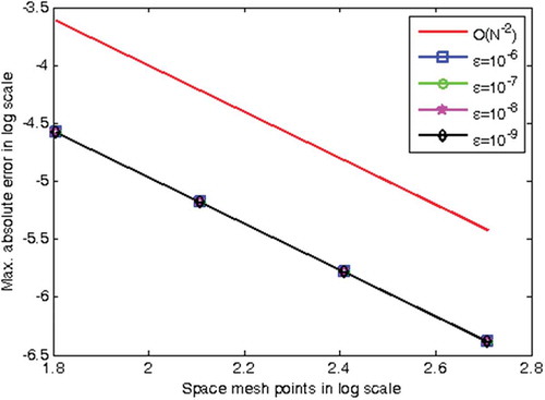
Figure 1. Log-log plot error for Example 1.2 with $N$ number of space mesh and $\mu ={10}^{-7}$

6. Discussion and conclusion

A numerical scheme is developed to solve a one-dimensional parabolic time-dependent convection-diffusion problem with two small perturbation parameters whose solution displays a parabolic layer. The method is developed in two steps, discretizing the time variable by the Crank-Nicholson method and the spatial variable by nonstandard finite difference method. We have established the consistency and stability of the proposed method to show its convergence. Using equally sized meshes, a parameter-uniform convergent scheme is obtained and it is observed to be in agreement with the result obtained by Munyakazi (2015). The validation of the theoretical analysis is done by taking two examples whose absolute maximum error of the solution is given in Tables 1 and 2. From tabular results, one can observe that as the value of the perturbation parameter approaches to zero the error goes constant. Furthermore, as the mesh size decreases the rate of convergence approaches to two, and the absolute maximum error decreases. These show that the solution of the scheme converges parameter uniformly (independent of the parameter) with the rate of convergence in agreement with the theoretical estimate.

Table 1. The maximum point-wise error and rate of convergence for example 1.1 where $\epsilon =2^{-5}$ and different values of $\mu$

$\mu \downarrow$	$N=32$	$N=64$	$N=128$	$N=256$	$N=512$
	$M=16$	$M=32$	$N=64$	$N=128$	$N=256$
Current method
$2^{-6}$	$2.4078e-04$	$6.0546e-05$	$1.5181e-05$	$3.7997e-06$	$9.5053e-07$
$2^{-8}$	$2.3648e-04$	$5.9390e-05$	$1.4884e-05$	$3.7252e-06$	$9.3180e-07$
$2^{-10}$	$2.3571e-04$	$5.9186e-05$	$1.4827e-05$	$3.7106e-06$	$9.2814e-07$
$2^{-12}$	$2.3551e-04$	$5.9135e-05$	$1.4814e-05$	$3.7073e-06$	$9.2729e-07$
$2^{-14}$	$2.3546e-04$	$5.9122e-05$	$1.4811e-05$	$3.7065e-06$	$9.2708e-07$
$\mathrm{P}\mathrm{r}\mathrm{a}\mathrm{b}\mathrm{a}$	$2.3545e-04$	$5.9119e-05$	$1.4810e-05$	$3.7063e-06$	$9.2703e-07$
$2^{-18}$	$2.3545e-04$	$5.9118e-05$	$1.4810e-05$	$3.7062e-06$	$9.2702e-07$
$2^{-20}$	$2.3545e-04$	$5.9118e-05$	$1.4810e-05$	$3.7062e-06$	$9.2702e-07$
$2^{-22}$	$2.3545e-04$	$5.9118e-05$	$1.4810e-05$	$3.7062e-06$	$9.2726e-07$
$2^{-24}$	$2.3544e-04$	$5.9118e-05$	$1.4810e-05$	$3.7062e-06$	$9.2713e-07$
$R$	1.9916	1.9958	1.9983	1.9991	1.9996
Method in Kadalbajoo and Yadaw (2012)
$2^{-6}$	$5.091e-3$	$4.580e-3$	$3.325e-3$	$2.004e-3$	$1.101e-3$
$2^{-8}$	$5.090e-3$	$4.327e-3$	$3.148e-3$	$1.898e-3$	$1.043e-3$
$2^{-10}$	$5.088e-3$	$4.265e-3$	$3.105e-3$	$1.873e-3$	$1.029e-3$
$2^{-12}$	$5.089e-3$	$4.250e-3$	$3.094e-3$	$1.866e-3$	$1.026e-3$
$2^{-14}$	$5.087e-3$	$4.246e-3$	$3.091e-3$	$1.865e-3$	$1.024e-3$
$2^{-16}$	$5.087e-3$	$4.245e-3$	$3.091e-3$	$1.864e-3$	$1.024e-3$
$2^{-18}$	$5.087e-3$	$4.245e-3$	$3.091e-3$	$1.864e-3$	$1.024e-3$
$2^{-20}$	$5.087e-3$	$4.245e-3$	$3.091e-3$	$1.864e-3$	$1.024e-3$
$2^{-22}$	$5.087e-3$	$4.245e-3$	$3.091e-3$	$1.864e-3$	$1.024e-3$
$2^{-24}$	$5.087e-3$	$4.245e-3$	$3.091e-3$	$1.864e-3$	$1.024e-3$
$R$	0.1527	0.4670	0.7302	0.8640	0.9314

Table 2. The maximum point-wise error and rate of convergence for example 1.2 where $\mu ={10}^{-7}$ and different values of $\epsilon$

$\epsilon \downarrow$	$N=64$	$N=128$	$N=256$	$N=512$
	$M=16$	$M=32$	$N=64$	$N=128$
Current method
${10}^{-6}$	$2.6377e-05$	$6.5877e-06$	$1.6474e-06$	$4.1182e-07$
${10}^{-7}$	$2.6377e-05$	$6.5877e-06$	$1.6474e-06$	$4.1182e-07$
${10}^{-8}$	$2.6377e-05$	$6.5877e-06$	$1.6474e-06$	$4.1182e-07$
${10}^{-9}$	$2.6377e-05$	$6.5877e-06$	$1.6474e-06$	$4.1182e-07$
$R$	$2.0014$	$1.9996$	$2.0001$	$1.9999$
Result in Gupta et al. (2019)
${10}^{-6}$	$3.8754e-5$	$1.0214e-5$	$2.6170e-6$	$6.6241e-7$
${10}^{-7}$	$3.8753e-5$	$1.0214e-5$	$2.6170e-6$	$6.6241e-7$
${10}^{-8}$	$3.8753e-5$	$1.0214e-5$	$2.6170e-6$	$6.6241e-7$
${10}^{-9}$	$3.8753e-5$	$1.0214e-5$	$2.5461e-6$	$6.6241e-7$
$R$	$1.9238$	$1.9646$	$1.9821$	$1.9910$
Result in Das and Mehrmann (2016)
${10}^{-6}$	$9.6949e-4$	$4.9906e-4$	$2.5231e-4$	$1.2824e-4$
${10}^{-7}$	$9.8712e-4$	$5.0049e-4$	$2.5485e-4$	$1.2853e-4$
${10}^{-8}$	$9.5128e-4$	$5.0026e-4$	$2.5237e-4$	$1.2781e-4$
${10}^{-9}$	$9.6746e-4$	$5.0012e-4$	$2.5461e-4$	$1.2804e-4$
$R$	$0.95193$	$0.97394$	$0.99186$	$0.99188$

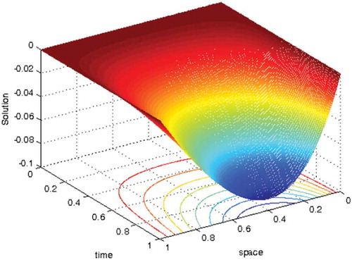
Numerical solution profiles are given in Figures 3 and 4 which show the geometrical appearance and property of the computed solution obtained by the proposed scheme. They confirm that the solution to the problem under investigation exhibits a parabolic type boundary layer. To show the relationship between the solution and the space variable, we have used the log-log plot in Figures 1 and 2 which is a straight line. This indicates the solution changes as a power of the space variable and the error is constant.

Figure 4. Numerical solution of Example 1.1 for $N=M=2^9,\epsilon =2^{-24}$ and $\mu =2^{-8}$

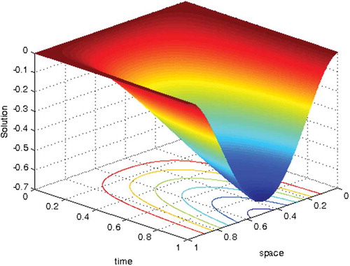
Figure 2. Log-log plot error for Example 1.1 with $N$ number of space mesh and $\epsilon =2^{-5}$

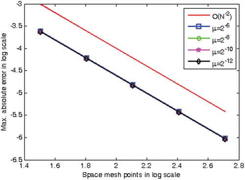
Figure 3. Numerical solution of Example 1.2 for $N=2^9,M=2^8,\epsilon ={10}^{-9}$ and $\mu ={10}^{-7}$

Both the theoretical and numerical analysis shows that the present method is second-order accurate and the convergence is parameter uniform. Further, it is observed that the formulated method is stable and consistent and gives more accurate results than some methods exist in the literature.

In a concise manner, the present method is simple and stable and convergent independent of the value of the perturbation parameter. Hence, the method is a good alternative method to solve problems of fluid flow where the Reynolds/Peclet number is sufficiently large.

List of Symbols

T	=	Maximum time value
M	=	Number of subintervals of the time domain
N	=	Number of subintervals of the space domain
k	=	Stepsize in the time direction
h	=	Stepsize in the space direction
$D_t^M$	=	Time mesh (the set of time nodes)
$D_x^N$	=	Space mesh (the set of space nodes)
TE1	=	Truncation error in the time direction
TE2	=	Truncation error in the space direction
C	=	Any generic constant independent of the perturbation parameters and the step sizes
U	=	The approximate solution to the analytical solution u
$E_{\epsilon ,\mu }^{N,M}$	=	Maximum pointwise error
R	=	Rate of convergence
Greek letters	=
$\epsilon$	=	Perturbation parameters multiplying the diffusion term
$\mu$	=	Perturbation parameters multiplying the convection term
${\tau }_1$	=	Reminder term of the Taylor series expansion in the time direction
$\alpha$	=	The smallest positive value of the convection coefficient on the given domain
${\gamma }^2$	=	Denominator function which replaces h2
$\xi$	=	Amplification factor

Additional information

Funding

The authors received no direct funding for this research.

Notes on contributors

Gemechis File Duressa

The research of the authors spans both on pure and applied mathematics. Much of their work has been focused on numerical solution of singular perturbation problems; finite difference methods, finite element methods, fitted operator and fitted mesh methods for solving singularly perturbed boundary value problem in ODEs and PDEs.

Gemechis File Duressa is an Associate Professor of Mathematics and faculty member of the Department of Mathematics, College of Natural Sciences at Jimma University. So far he has published more than 50 research articles in reputable journals.

Tariku Birabasa Mekonnen is a Ph.D. Scholar at the Department of Mathematics, College of Natural and Computational Sciences, Wollega University, Nekemte, Ethiopia.

References

- Belhocine, A. (2016). Numerical study of heat transfer in fully developed laminar flow inside a circular tube. The International Journal of Advanced Manufacturing Technology, 85(9–12), 2681–16. DOI: 10.1007/s00170-015-8104-0
- Belhocine, A. (2017). An approximate numerical solution to the Graetz problem with constant wall temperature. International Journal of Computing Science and Mathematics, 8(1), 35–51. https://doi.org/10.1504/IJCSM.2017.083126
- Belhocine, A., & Wan Omar, W. Z. (2017). An analytical method for solving exact solutions of the convective heat transfer in fully developed laminar flow through a circular tube. Heat Transfer-Asian Research, 46(8), 1342–1353. https://doi.org/10.1002/htj.21277
- Bullo, T., Duressa, G., & DEGLA, G. (2019). Higher order fitted operator finite difference method for two-parameter parabolic convection-diffusion problems. International Journal of Engineering and Applied Sciences, 11(4), 455–467. https://doi.org/10.24107/ijeas.644160
- Chandru, M., Prabha, T., Das, P., & Shanthi, V. (2019). A numerical method for solving boundary and interior layers dominated parabolic problems with discontinuous convection coefficient and source terms. Differential Equations and Dynamical Systems, 27(1–3), 91–112. https://doi.org/10.1007/s12591-017-0385-3
- Clavero, C., Gracia, J. L., Shishkin, G. I., & Shishkina, L. P. (2017). An efficient numerical scheme for 1d parabolic singularly perturbed problems with an interior and boundary layers. Journal of Computational and Applied Mathematics, 318, 634–645. http://dx.doi.org/10.1016/j.cam.2015.10.031
- Das, P., & Mehrmann, V. (2016). Numerical solution of singularly perturbed convection-diffusion-reaction problems with two small parameters. BIT Numerical Mathematics, 56(1), 51–76. https://doi.org/10.1007/s10543-015-0559-8
- Gupta, V., Kadalbajoo, M. K., & Dubey, R. K. (2019). A parameter-uniform higher order finite difference scheme for singularly perturbed time-dependent parabolic problem with two small parameters. International Journal of Computer Mathematics, 96(3), 474–499. https://doi.org/10.1080/00207160.2018.1432856
- Jha, A., & Kadalbajoo, M. K. (2015). A robust layer adapted difference method for singularly perturbed two-parameter parabolic problems. International Journal of Computer Mathematics, 92(6), 1204–1221. https://doi.org/10.1080/00207160.2014.928701
- Kadalbajoo, M., & Yadaw, A. S. (2012). Parameter-uniform finite element method for two-parameter singularly perturbed parabolic reaction- diffusion problems. International Journal of Computational Methods, 9(4), 1250047. https://doi.org/10.1142/S0219876212500478
- Kadalbajoo, M. K., & Jha, A. (2012). Exponentially fitted cubic spline for two-parameter singularly perturbed boundary value problems. International Journal of Computer Mathematics, 89(6), 836–850. https://doi.org/10.1080/00207160.2012.663492
- Khandelwal, P., & Khan, A. (2017). Singularly perturbed convection- diffusion boundary value problems with two small parameters using non- polynomial spline technique. Mathematical Sciences, 11(2), 119–126. https://doi.org/10.1007/s40096-017-0215-3
- Liu, J.-G., Yang, X.-J., & Feng, -Y.-Y. (2019). On integrability of the time fractional nonlinear heat conduction equation. Journal of Geometry and Physics, 144, 190–198. https://doi.org/10.1016/j.geomphys.2019.06.004
- Liu, J.-G., Yang, X.-J., Feng, -Y.-Y., & Zhang, H.-Y. (2020). On the generalized time fractional diffusion equation: Symmetry analysis, conservation laws, optimal system and exact solutions. IJGMM, 17(1), 2050013–2050028. DOI: 10.1142/S0219887820500139
- Mickens, R. E. (2000). Applications of nonstandard finite difference schemes. World Scientific.
- Mickens, R. E. (2005). Advances in the applications of nonstandard finite difference schemes. World Scientific.
- Munyakazi, J. B. (2015). A robust finite difference method for two-parameter parabolic convection-diffusion problems. Applied Mathematics & Information Sciences, 9(6), 2877. http://dx.doi.org/10.12785/amis/090614
- O’Riordan, E., Pickett, M., & Shishkin, G. (2006). Parameter-uniform finite diffusion schemes for singularly perturbed parabolic diffusion-convection- reaction problems. Mathematics of Computation, 75(255), 1135–1154. https://doi.org/10.1090/S0025-5718-06-01846-1
- O’Riordan, E., Pickett, M. L., & Shishkin, G. I. (2003). Singularly perturbed problems modeling reaction-convection-diffusion processes. Computational Methods in Applied Mathematics, 3(3), 424–442. https://doi.org/10.2478/cmam-2003-0028
- Patidar, K. C. (2008). A robust fitted operator finite difference method for a two-parameter singular perturbation problem1. Journal of Difference Equations and Applications, 14(12), 1197–1214. https://doi.org/10.1080/10236190701817383
- Phaneendra, K., and Mahesh, G. (2017). Solution of two parameters singular perturbation problem using higher order compact numerical method. Global and Stochastic Analysis, 4(2), 225–236. https://www.mukpublications.com/resources/6.%20PHANEENDRA.pdf
- Ramos, J. I. (2005). An exponentially-fitted method for singularly perturbed, one-dimensional, parabolic problems. Applied Mathematics and Computation, 161(2), 513–523. https://doi.org/10.1016/j.amc.2003.12.046
- Roos, H.-G., & Uzelac, Z. (2003). The Sdfem for a convection-diffusion problem with two small parameters. Computational Methods in Applied Mathematics, 3(3), 443–458. https://doi.org/10.2478/cmam-2003-0029
- Vulanović, R. (2001). A higher-order scheme for quasilinear boundary value problems with two small parameters. Computing, 67(4), 287–303. https://doi.org/10.1007/s006070170002
- Zahra, W., & El Mhlawy, A. M. (2013). Numerical solution of two- parameter singularly perturbed boundary value problems via exponential spline. Journal of King Saud University-Science, 25(3), 201–208. https://doi.org/10.1016/j.jksus.2013.01.003
- Zahra, W., El-Azab, M., & El Mhlawy, A. M. (2014). Spline difference scheme for two-parameter singularly perturbed partial differential equations. Journal of Applied Mathematics & Informatics, 32(1_2), 185–201. https://doi.org/10.14317/jami.2014.185