The Hydroacoustic Network of the CTBT International Monitoring System: Access and Exploitation

ABSTRACT

The hydroacoustic network of the International Monitoring System for verifying compliance with the Comprehensive Nuclear-Test-Ban Treaty consists of six hydrophone array stations and five land-based seismic stations for recording T-phases. We provide a comprehensive overview of the network with details of the station configurations and data accessibility. Since 2014, data from all stations on the territory of Australia, the United Kingdom and the United States of America (four hydrophone arrays and one T-phase station) have been freely available, and we demonstrate how this data can be obtained and displayed with openly available software and minimal amounts of code. We detail which open seismic stations may act as limited surrogates for closed IMS stations. We demonstrate how the most fundamental characteristics of the hydroacoustic data can be obtained using open software, and we advocate extensive exploitation of this data for interpreting both hydroacoustic and converted seismic signals. We demonstrate signals from the 2017 North Korean nuclear test on both seismic and hydrophone data. Optimizing procedures using the open data allows us to explore the likely capability for all stations, even if real-time detection and processing outside the CTBT system is currently limited to hydrophone stations HA01, HA08, HA10 and HA11.

KEYWORDS:

• CTBT
• IMS
• open data
• hydroacoustic
• DPRK
• test-ban-treaty monitoring

Introduction

The verification regime for the Comprehensive Nuclear-Test-Ban Treaty (CTBT) includes networks of sensors for four distinct technologies: radionuclide, seismic, infrasound and hydroacoustic. These sensor networks, together with radionuclide laboratories, constitute the International Monitoring System or IMS. The seismic, infrasound and hydroacoustic networks detect signals in the solid earth, atmosphere and oceans which could be generated by an explosion, and the radionuclide network exists to verify the nuclear nature of an event detected and located by the other technologies: the so-called waveform technologies. It is an oversimplification to say that the seismic, infrasound, and hydroacoustic networks exist to detect respectively underground, atmospheric, and underwater nuclear tests. The solid earth, oceans, and atmosphere constitute a coupled system with wave interactions between the different domains and many events, both natural and anthropogenic, are recorded by two or all three of the waveform technologies. The data recorded by these sensors is transmitted in near-real-time to the International Data Center (IDC) in Vienna where it is collected and analyzed.

IMS data is made available to State Parties through their National Authorities but is owned by the State Party that hosts the station. The treaty text (CTBTO 1996) states (Article II, Paragraph 7) that “Each State Party shall treat as confidential and afford special handling to information and data that it receives in confidence from the Organization in connection with the implementation of this Treaty”. This has the consequence that IMS data is, in general, not available to the general public; the only exceptions to this are when the host State Party actively makes data openly available. Recognizing the value that much of the IMS data has for broader scientific purposes has resulted in some advances in making data available. Access to all IMS data is possible via the vDEC or virtual Data Exploration Center (https://www.ctbto.org/specials/vdec/) but this requires submitting an application and signing a contract which sets strict conditions for the use of data, for example, that it can only be used for exactly the purpose specified in the application, and that raw data cannot be redistributed. Data obtained via the vDEC is also necessarily archive data and this precludes, for example, processing of the data in near-real-time. Much IMS data is made available to the general public directly from the host State Party, sometimes through the designated National Data Center (NDC) and sometimes through third-party data repositories. In this paper, we focus on the hydroacoustic component of the IMS and investigate what data the network consists of and which part of it is openly available. The interactive map at https://www.ctbto.org/map/ provides an overview of the locations of stations for the different technologies, but there is insufficient information here alone to allow a user outside the CTBT system to know the extent of the data and find out how it is obtained. There are, however, other open resources which contain this information and our aim here is to collect this information in one place.

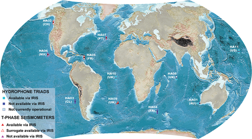
Oceanic sound can travel global distances with minimal loss in the so-called SOFAR (Sound Fixing and Ranging) or Deep Sounding channel, at which the speed of sound is a minimum. This is typically at a depth of approximately 750 m below the sea surface. The hydroacoustic network comprises 11 stations as displayed in Figure 1. There are two types of stations: hydrophone arrays and T-phase stations. The former consist of one or two triads of hydrophones submerged directly in the SOFAR channel. The latter consist of pairs of three-component seismic stations deployed close to steep-sloping coastlines to record so-called T-phases: seismic body waves generated when the hydroacoustic wave meets land at depth. These stations are called T-phase stations (T standing for Tertiary, in a naming convention consistent with P, primary, and S, secondary, seismic waves). There are qualitative differences between the two types of stations:

• The hydrophones measure the pressure wave directly in the SOFAR channel, whereas the T-phase stations rely on a conversion in which energy is lost.

• The hydrophone triads are arrays which can measure phase velocity, direction and coherence, and help determine from where a wave has arrived. In principle, particle motion can help identify a T-phase but, since it is a seismic body wave, unambiguous identification may require considerable work, experience and skill.

Figure 1. The hydroacoustic component of the International Monitoring System (IMS) for monitoring compliance with the Comprehensive Nuclear-Test-Ban Treaty (CTBT). There are six hydrophone stations and five so-called T-phase stations.

The rationale behind the deployment of the T-phase stations is given by Okal (2001) and Stevens et al. (2001), Stevens et al. (2021) model both the hydroacoustic propagation and the conversion to seismic body waves at the T-stations. The advantages of the hydrophone stations come at a cost; the cost of deploying and maintaining these stations dwarfs the cost of deploying T-phase seismic stations.

The Incorporated Research Institution for Seismology (or IRIS) stores and redistributes waveform data for research purposes. Except for data under a temporary embargo, as is typical for field deployments where a project has paid for the deployment and operation of stations, all data available from IRIS are open to all users with no pre-conditions. All data at IRIS are arranged according to network as specified by a two-letter code as assigned through membership of FDSN, the Federation of Digital Seismic Networks (https://www.fdsn.org/). In recent years, IRIS has stored seismic, infrasound and hydroacoustic data under the code IM (International Miscellaneous) including IMS data offered by State Parties willing to share their data openly in this way. The map obtained through https://ds.iris.edu/gmap/#network=IM&planet=earth shows the locations of all sites recorded under this network code. Not all of the sites displayed indicate that data from a particular station is openly available but, for the IMS hydroacoustic stations HA01, HA08, HA09, HA10 and HA11, this data is indeed open and clicking on a given site will provide information about the time history and holdings of the station (e.g. https://ds.iris.edu/mda/IM/H08S2/?starttime=2002-01-17&endtime=2599-12-31). Observing the naming conventions applied, it was possible to identify the locations of all sites through the station registry of the International Seismological Center (ISC). This applied to both hydrophone and T-phase stations, including those not currently generally available. We will provide an overview of the locations and configurations of all stations.

In addition to open data, scientific progress has advanced through the availability of easy-to-apply open-source software. The ObsPy package (https://pypi.org/project/obspy/) allows direct access to waveforms stored at IRIS and other data sources using only a few lines of code. We provide examples of how to load and display open IMS hydroacoustic data using obspy. The instant access that this software provides for those stations that are made openly available lowers the threshold for investigating data for the presence of signals. A user that asks “Is a signal visible on this station for this event?” can answer that question within seconds for the open stations. Even though the vDEC may provide access to data for the closed stations, the threshold for applying is high. Array processing is central to the interpretation of hydrophone data, and we demonstrate the application of free software made available by the University of Alaska, Fairbanks. With the station overviews and data examples, it is our intention to raise awareness of this source of data and encourage exploitation to a wide range of applications, both within test ban treaty monitoring and more generally.

Methodology

We search the publicly available information on the IMS hydroacoustic network from the CTBTO website, the IRIS website, and the International Seismological Center and summarize what data is available to persons with no association with the CTBTO or National Data Centers. We search the websites of providers of open software for means to obtain and analyze the openly available data. We describe what is necessary to access the data that is not currently open via the CTBTO vDEC (virtual Data Exploration Center) and the conditions that are attached.

The Hydroacoustic Network

Table 1 provides the registered coordinates for all the sites of the six hydrophone stations. However, the coordinates for HA03 are valid only for data until 2010 as this station was re-established in 2014 after it had been rendered inoperable by the tsunami generated by the large Chilean earthquake of 2010. The coordinates of the HA03 hydrophones installed in 2014 are available through the vDEC to registered users. The HA04 coordinates listed in the table are to be considered only as nominal and are different from those of the hydrophones certified in 2017. The accurate HA04 coordinates are also available through vDEC to registered users. We note that, unlike seismic stations, hydrophones may experience a drift of location with time and, at the IDC, the exact locations are continually updated through empirical calibrations. The most up-to-date coordinates for all hydrophone stations are available through the vDEC to registered users.

Table 1. Stations of the IMS hydrophone network. All stations consist of two sets of hydrophone triads except for HA01 with only a single hydrophone triad. We indicate the open availability of data and the names of the closest open seismic stations. Note that the coordinates provided are those registered in the International Seismological Center’s station registry and have changed for some stations (see text). Unlike seismic stations which are fixed in the solid earth, hydrophones are subject to drift and the exact coordinates are continually calibrated and recalculated. Up-to-date coordinates are available via the virtual Data Exploration Center (vDEC).

Station	Registered coordinates. (See text for additional notes)			IRIS availability	Nearest open seismic stations	Station name
	Site	Latitude	Longitude
HA01	H01W1	−34.8930	114.1540	IM(2014-12-12)	IU.NWAO	Cape
(AU)	H01W2	−34.8985	114.1338	AU(2019-10-14)	AU.RKGY	Leeuwin
	H01W3	−34.8832	114.1361
	H03N1	−33.4412	−78.9120
	H03N2	−33.4399	−78.9324			Juan
HA03	H03N3	−33.4556	−78.9240	Not	C1.VA04	Fernandez
(CL)	H03S1	−33.8437	−78.9058	available		Islands
	H03S2	−33.8370	−78.9262
	H03S3	−33.8258	−78.9095
	H04N1	−46.1608	51.7792
	H04N2	−46.1644	51.8025
HA04	H04N3	−46.1772	51.7832	Not	G.CRZF	Crozet
(FR)	H04S1	−46.8409	51.9130	available		Islands
	H04S2	−46.8536	51.8935
	H04S3	−46.8354	51.8870
	H08N1	−6.3421	71.0143	Not
	H08N2	−6.3251	71.0001	operational
HA08	H08N3	−6.3454	70.9919		II.DGAR	Diego
(UK)	H08S1	−7.6453	72.4744			Garcia
	H08S2	−7.6453	72.4933	IM(2014-12-12)
	H08S3	−7.6275	72.4838
	H10N1	−7.8457	−14.4802
	H10N2	−7.8278	−14.4875
HA10	H10N3	−7.8409	−14.5017	IM(2014-12-11)	II.ASCN	Ascension
(UK)	H10S1	−8.9412	−14.6484			Island
	H10S2	−8.9591	−14.6453
	H10S3	−8.9527	−14.6629
	H11N1	19.7136	166.8911
	H11N2	19.7311	166.8968
HA11	H11N3	19.7179	166.9099	IM(2014-12-11)	IU.WAKE	Wake
(US)	H11S1	18.5083	166.7003			Island
	H11S2	18.4905	166.7054
	H11S3	18.4949	166.6873

The stations’ locations are displayed, together with the topobathymetric context, in Figure 2. Station HA01 has a central hub at Cape Leeuwin on mainland Australia with a single triad of hydrophones approximately 100 km to the southwest. This distance from shore is needed to attain the necessary depth in the SOFAR channel. All the remaining stations have central hubs situated on islands and a pair of hydrophone triads, one to the north and one to the south of the island or archipelago. We see in Figure 2 how the water depths surrounding the island hubs vary and the consequences that this has for the locations of the hydrophone triads with respect to their land-based hubs. This has, in turn, consequences for logistics and the cost of deployment. The island and shallow bathymetry typically block the propagation of oceanic sound and this is the basis for placing a hydrophone triad on either side of an island.

Figure 2. Geometries of the 6 hydrophone array stations and locations with respect to the closest open seismic stations. Each of the hydrophone triads forms an approximate equilateral triangle of sensors with around 2 km from sensor to sensor. The scales vary slightly from panel to panel in an attempt to provide the most useful contextual picture of the stations in relation to their topobathymetric surroundings.

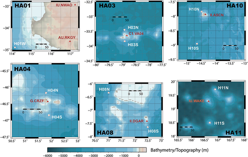
The bathymetric constraints at HA08 are exceptionally complicated, and the northern triad is over 200 km to the northwest of the southern triad. At the time of writing, the northern triad has been inoperational for many years, with both logistical and political barriers to making it operational again. While operational, data from the northern triad had been used for purposes ranging from earthquake observation (e.g. Hanson and Bowman 2006) to monitoring marine mammals (e.g. Cerchio et al. 2020). The southern triad is still operational. It is on the right side of the bathymetric barrier (Pulli and Upton 2002) to observe sound from earthquakes to the East and was used by Tolstoy and Bohnenstiehl (2005) and Guilbert et al. (2005) to track the rupture of the 26 December 2004 great Sumatra-Andaman earthquake.

The different panels of Figure 2 indicate that the island or shallow bathymetry does not always mean that sound is blocked from one or the other hydrophone triad. There are clearly many directions from which signals propagating towards HA10 (Ascension Island) or HA11 (Wake Island) would be detected on both sets of triads, further increasing confidence in any association of signals with a potential source.

We note that all the hydrophone arrays are near fully open seismic stations which may act as a proxy for the hydrophone array. This applies to the two hydrophone stations which are not open (HA03 and HA04) and all the hydrophone stations prior to December 2014. Stevens et al. (2021) provide direct comparisons between hydroacoustic signals on station HA10 and the corresponding T-phases observed on the seismic station II.ASCN. A clear T-phase visible on the seismic stations C1.VA04 or G.CRZF may indicate that hydrophone data from HA03 or HA04 is worth investigating for the relevant time interval. The station HA01 was transferred from the IM network to the AU network (Geoscience Australia) in 2019. This does not have any consequences for access to the data other than that the correct network code must be specified for the requested time period. (Indeed, a wild card can usually be specified in place of the network code.)

Table 2 and Figure 3 present the locations and contexts of all the T-phase stations. H09N1 and H09W1 on the island of Tristan da Cunha have both been open since December 2014 and the GEOSCOPE station G.TRIS may act as a surrogate T-phase station even further back in time. The stations HA02 and HA05 are not available via IRIS, but the stations CN.VIB, CN.DIB, WI.DSD and WI.MPOM are almost co-located with H02N1, H02S1, H05N1 and H05S1, respectively, so close that the waveforms are likely to be almost identical if the different instrument responses are accounted for. HA06 and HA07 (Socorro, Mexico and Flores, Portugal) are unique in not having, to the best of our knowledge, surrogate open stations. Stations HA02 and HA05 have many other open seismic stations relatively close (not displayed).

Figure 3. Geometries of the 5 T-phase stations. Stations with names in red are almost co-located with the CTBT T-phase stations and are freely available from IRIS. H09N1 and H09W1 are also open. The scales vary slightly from panel to panel in an attempt to provide the most useful contextual picture of the stations in relation to their topobathymetric surroundings.

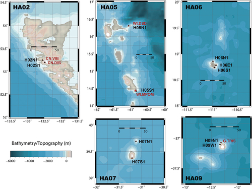
Table 2. Seismic stations of the IMS T-phase network. A surrogate station means a seismic station in the immediate vicinity of the CTBT station which has openly available data and for which the data is likely to closely resemble that on the CTBT station.

Station	Site	Latitude	Longitude	IRIS availability	Open surrogate station (IRIS)	Name
HA02	H02N1	53.2519	−132.5419	Not available	CN.VIB (2005-09-23)	Van Inlet
(CN)	H02S1	53.2025	−132.4766		CN.DIB (2005-09-23)	Dawson Inlet
HA05	H05N1	16.3164	−61.0567	Not available	WI.DSD (2013-01-01)	Guadeloupe
(FR)	H05S1	14.4250	−60.8367		WI.MPOM (2013-05-2)	Martinique
HA06	H06N1	18.8616	−110.9861	Not available	None	Socorro
(MX)	H06S1	18.7347	−110.9575
	H06E1	18.7805	−110.9253
HA07	H07N1	39.6912	−31.1196	Not available	None	Flores
(PT)	H07S1	39.3786	−31.2061
HA09	H09N1	−37.0681	−12.3152	IM(2014-12-18)	G.TRIS	Tristan
(UK)	H09W1	−37.0972	−12.3350		(2004-03-03)	Da Cunha

Processing Examples

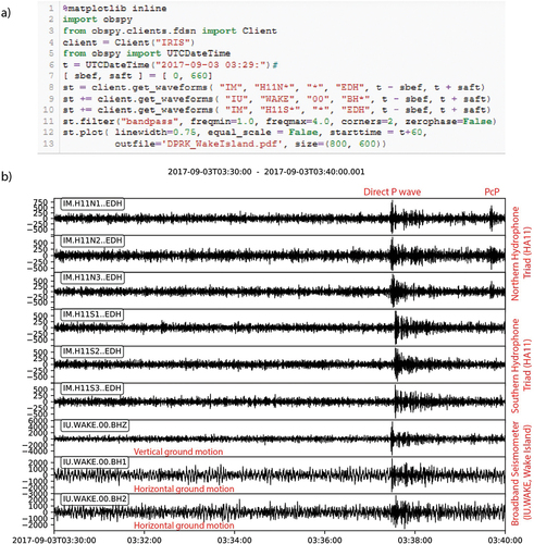
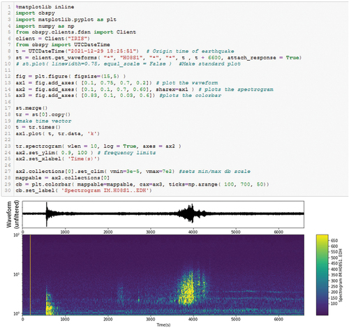
Obspy provides a means of reading in data segments using only a few lines of python code. Figure 4(a) shows a 13-line segment of code which reads in and plots a 10-minute-long segment of waveform data from the hydrophone triads of station HA11 (Wake Island) together with the corresponding data from the open broadband seismometer IU.WAKE. Figure 4(b) shows an annotated display of what this code segment generates. The waveform plot begins at a time 03:30 UTC on 3 September 2017: the time at which North Korea carried out its sixth and largest nuclear test. The Punggye-ri nuclear test site is about 4300 km from the station IU.WAKE and the direct seismic P-wave takes 7 minutes, 25 seconds to reach the station. The signal is the clearest on the channel IU.WAKE.00.BHZ which records vertical ground motion. The BH1 and BH2 channels are horizontal sensors at right angles to each other. The signal is also visible on these channels but is less clear against the background noise. What may come as a greater surprise is that the P-wave is clearly recorded on all six of the hydrophone sensors: a seismic wave in the solid earth resulting in a pressure wave in the water. An inspection of the International Seismological Center bulletin entry for this event shows that the P-wave arrivals at the sensors H11S1, H11S2 and H11S3 are in fact used to constrain the event location. The sensors H11N1, H11N2 and H11N3 are not used in this solution. A second signal is visible on the northern triad of hydrophones 2 minutes after the first P-wave arrival. The time of this arrival corresponds with the time we would expect to see PcP, the P-wave that has dived down and rebounded off the Core-Mantle-Boundary. The PcP arrival is not visible on either the southern triad or the IU.WAKE station.

Figure 4. Ten minutes of data from the seismic station IU.WAKE and the two hydrophone triads of the station HA11 (Wake Island) following the 3 September 2017, DPRK nuclear test. The short code sequence required to generate the plot is displayed in panel (a) and an annotated image of the result is displayed in panel (b) with the added text in red.

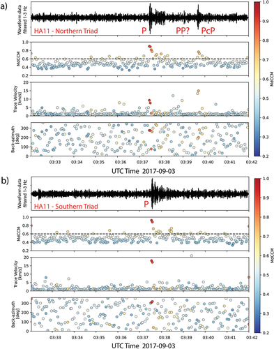
As the two hydrophone triads are minimal array stations, we are able to measure the small time delays between the signals on the different sensors to estimate the direction and the speed at which the wavefront crosses the station. (We use the word minimal since 3 is the minimum number of sensors needed to do this.) This is useful for associating a signal with a source and for determining what kind of signal it is. Does it travel with the speed of a seismic wave or with the speed of a water wave? The University of Alaska, Fairbanks, has developed free software which measures and displays the speed and direction of wavefronts crossing arrays (link provided in the data availability statement). The software was developed for infrasound arrays, but the exact same algorithm can be applied to the hydrophone data. The outcome of this software applied to the North Korean seismic signal on the hydrophone arrays is displayed in Figure 5. The high values of the parameter labelled MdCCM, with the associated red colors, indicate that the signals on the different sensors are very similar at a given moment: that they are coherent across the array. The time of the P-wave arrival for both hydrophone triads is associated with high coherence, a high trace velocity (consistent with the apparent velocity of a seismic P-wave), and a direction of about 300 degrees, pointing back towards the North Korean nuclear test site. Figure 5 confirms our identification of this as being a seismic P-phase from this event transferred into the water column. The identification of the PcP phase on the northern triad is also supported by high coherence, high phase velocity, the frequency content and an appropriate direction. Its visibility on the northern triad is as surprising as its absence on the seismometer and the southern hydrophone triad. This is the result of heterogeneity (or roughness) in the solid earth. The observation of PcP is less predictable than the observation of P as there are more places in the mantle where it may be deflected away or attenuated (e.g. Gassner et al. 2015, and references therein). It is likely such a deflection that leads to its non-observation of PcP at the WAKE seismometer or the southern hydrophone triad of HA11. Its observation at H11N is worthy of note. A possible PP phase (a P phase that has bounced off Earth’s surface between the source and station) is seen but it is not strong enough to be confirmed by array measurements, and so we leave a question mark at this small signal.

Figure 5. Properties of the pressure field in the hydrophone data estimated using correlation analysis between the traces on the different hydrophone sensors. MdCCM measures the coherence between the signals on the different sensors. The trace velocity or apparent velocity is how fast the wave appears to cross the array. The trace velocity for a hydroacoustic phase would be around 1.5 km/s, about ten times slower than the trace velocities observed here. The back-azimuth is the direction, moving clockwise from the North from which the wave arrives. The timing, speed and direction of the signals indicates that they are consist with converted seismic signals from the North Korean nuclear test. A window length of 5 seconds, and a filter 1–3 Hz was applied. The dashed line for MdCCM = 0.6 is an arbitrarily chosen threshold value.

Figures 4 and 5 show only seismic phases, not true hydroacoustic phases. Zampoli et al. (2021) display the converted seismic signals from this underground nuclear explosion on several of the hydrophone triads. In addition, they show evidence of a weak tertiary phase detected at HA11 together with a possible excitation mechanism for this arrival.

Figure 6 shows a far longer segment of hydrophone data at station HA08 at the time of a large earthquake. We see the impulsive seismic P-wave arrival about nine and a half minutes after the earthquake and this is followed over an hour later by a signal which emerges out of the noise. Figure 6 also displays a so-called spectrogram which indicates energy in the seismic signal as a function of both time and frequency. Spectrograms (or sonograms) are a very typical means of displaying hydroacoustic data as signals of interest frequency occupy very specific frequencies and can often change in both frequency and time. We see that the seismic signal is focused at far lower frequencies (1–4 Hz) than the subsequent hydroacoustic signal (5–15 Hz). We also see a signal at about 2300 seconds in the spectrogram which is difficult to see in the waveform data. Figure 6 also displays all the code needed to generate the plot in a Jupyter notebook.

Figure 6. Hydrophone trace and spectrogram for station HA08 almost two hours following a magnitude 7.3 earthquake in Indonesia (https://earthquake.usgs.gov/earthquakes/eventpage/us7000g7lx/executive). The code displayed above is sufficient to generate the image displayed.

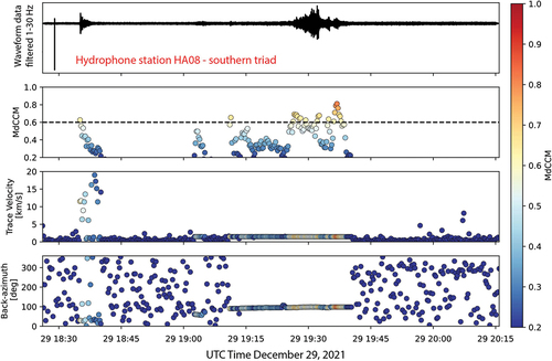
We apply the array processing software also to this segment of data and display the outcome in Figure 7. In Figure 5, we wanted to measure the speed and direction of a rather short-duration signal in a low-frequency band. With a 5-second window length in the 1–3 Hz frequency band, we have a relatively low time bandwidth product and so the coherence measure, MdCCM, was relatively high at many points with no clear signals. In Figure 7, we process a much longer data segment with a much wider frequency band. With this higher time-bandwidth product, it is far more difficult for the signals on the different sensors to resemble each other by sheer coincidence; a high coherence value is far more likely to indicate a common cause. The earthquake is approximately 6000 km east of the station and if we assume a sound speed of approximately 1500 m/s, then we would expect a direct sound wave to arrive at around 4000 seconds. From Figure 6 we see that this is when the maximum amplitude is achieved, close to the end of the wavetrain. For many minutes before this time, coherent energy has arrived at the station with a water sound speed and from directions similar to that of the earthquake. The seismic waves radiate out from the location of the earthquake and generate tertiary phases in the ocean at interfaces between the solid earth and water, located between the source and receiver. T-waves that are generated at interfaces closer to the receiver than the earthquake itself will arrive before the direct waves as they propagate shorter distances in the medium with the slower wave speed. It is possible to map out accurately the origins of such sound waves, including reflections that arrive much later than the direct waves (e.g. Upton et al. 2006).

Figure 7. Properties of the hydroacoustic wavefield at station HA08 following the Indonesia earthquake using correlation analysis. We see clear differences between the converted seismic arrival (fast-arriving, short duration, high trace velocity) and the true hydroacoustic signal (slow-arrival, long duration, low trace velocity). A window length of 30 seconds, and a filter 1–30 Hz was applied. The dashed line for MdCCM = 0.6 is an arbitrarily chosen threshold value.

We note that the resolution in trace velocity and direction is far higher on the hydrophone triads for the hydroacoustic signal than for the seismic phases. With approximately 2 km between the sensors, the time-delay for a hydroacoustic wave arrival on two sensors can exceed a second. A teleseismic wave, like that displayed in Figures 4 and 5, travels much faster and, due to the angle of incidence, covers the ground with about 15 km/s: 10 times faster than the hydroacoustic signal. Compounded by the lower and more limited frequency content of the seismic signal, we will have far less accuracy in our estimate of phase velocity and direction for the seismic signal than for the hydroacoustic signal.

The software used to generate Figures 5 and 7 makes almost no assumptions about the data, beyond the window length and the frequency band specified. This means that we can implement a coherence-based detector using a recipe based on this software for the six open-access hydrophone triads (H01W, H08S, H10S, H10N, H11S, H11N) in near-real-time. This will allow us to report times of coherent energy, together with signal amplitude, frequency content, phase velocity and azimuth and alert us to interesting signals almost as they arrive at the stations. Such a process is not possible for stations HA03 and HA04 for users not specifically authorized within the CTBT system. It should also be noted that Iezzi et al. (2022) describe a published extension of the software used here which processes the waveform data in multiple narrow frequency bands simultaneously. This extension obviates the need to specify a pre-defined frequency band and can detect, characterize and display arrivals occupying different parts of the frequency spectrum in the same way as the PMCC (Progressive Multichannel Cross Correlation) software employed at the IDC.

Conclusions and Recommendations

We have provided a comprehensive overview of the stations of the hydroacoustic network of the IMS and have displayed their locations in a topobathymetric context and provided details on which are openly accessible. We have identified which open seismic stations are closest to the hydroacoustic stations (both hydrophone stations and T-phase sites). For those stations that are not openly available, we have provided details of where to apply for access via the CTBTO virtual Data Exploration Center (vDEC). Indeed, some excellent science has been carried out using the IMS hydroacoustic data in this way (e.g. Metz et al. 2016). However, there are serious limitations to what can and cannot be done with data acquired via the vDEC and exploration and experimentation is far easier for those stations which are currently truly open. We point out in particular that continuous processing can be carried out on the open stations in near-real-time, providing alerts to any signals of interest almost as soon as they are recorded. We have applied array processing using fully open software on hydrophone data and demonstrated seismic signals from an earthquake and a nuclear explosion, and hydroacoustic signals generated by an earthquake. The recipes demonstrated can be applied to all the hydrophone stations at all times and can be used to display signals from all kinds of sources.

All the data accesses illustrated in this paper were carried out in January and February 2022. Like all aspects of technology, and systems subject to political decisions, there are no guarantees that the systems demonstrated in this paper will be valid at any time in the future. The open availability of IMS waveform data is decided by State Parties: not the CTBTO. In the future, more data may be made openly available if so decided by the host State Party. Similarly, the provision of data to IRIS from the Australian, UK and US stations which has occurred since 2014 could stop at any time if the host State Party should decide so. At the time of writing, there is likely to be a merger in the near future between IRIS and UNAVCO (previously The University NAVSTAR Consortium, https://www.unavco.org/). This is not likely to change the availability of data currently held by IRIS but, with an organizational change, this may mean that the procedures applied to access the data will change. The best defence a researcher has against the procedures described here becoming obsolete is to engage as closely as possible with the organizations and research communities. The python programming language and associated packages are in continual evolution and, just as the scripts displayed did not exist 15 years ago, the procedures described are likely to have been replaced by something else in the not-too-distant future. While the locations of the stations are fixed in the CTBT treaty text, the stations are subject both to the forces of nature and political interventions. The station HA03 became inoperational following a tsunami in 2010 and was reinstalled in 2014 (CTBTO 2014). The northern triad of station HA08 has been out of operation for many years, and its re-establishment is subject to both logistical and political hurdles.

We have not touched on the physics of oceanic sound propagation. The oceans are a time-dependent propagation medium and modelling the paths and propagation times of hydroacoustic waves is a highly complicated field (see, for example, the analyses of the 2017 events in the South Atlantic Ocean discussed by Heyburn, Bowers, and Green 2020; Vergoz et al. 2021 and references therein). The most fundamental properties of the hydrophone data can be discretized in time series and tensors, e.g. energy as a function of time and frequency (as in Figure 6) or as trace velocity, direction and coherence (as in Figure 7). This makes the post-processed data very amenable to pattern recognition and machine learning (see Bianco et al. 2019 for a comprehensive overview of machine learning in acoustics). We hope that this overview has motivated the investigation of this rich and unique dataset by researchers and computer scientists who otherwise may not be aware of what is available. We also hope that the maps will provide some impression of the dimensions of the infrastructure necessary to support these stations which will, in turn, lead to an increased appreciation of the value of this data. As Sato (2021) points out, civil and scientific applications will help strengthen and sustain the verification regime. Increased exploitation and application of International Monitoring System data will help ensure its continuity, and we hope that this overview will help to increase awareness of, and familiarity with, this valuable component of the system.

Acknowledgments

I am very grateful to Robert Porritt, Thomas Lecocq, Koen van Noten and Sven Peter Näsholm for advice and guidance on displaying data using ObsPy and matplotlib.

The existence of this data is due to to an enormous collective investment through the CTBTO system, and I am grateful to all station operators, CTBTO staff and all involved in the installation and maintenance of these stations.

I extend my enormous gratitude to IRIS for facilitating access to this data and to the national authorities of Australia, the United Kingdom and the United States for allowing this data to become freely available.

I am grateful to two reviewers for thorough and detailed comments that have improved this manuscript significantly.

Disclosure Statement

No potential conflict of interest was reported by the author(s).

Data Availability Statement

An interactive map with all parts of the International Monitoring System is found at https://www.ctbto.org/map/ and the designations of hydrophone and T-phase stations are found in the treaty text (https://www.ctbto.org/the-treaty/treaty-text/) on page 115 of the PDF document on https://www.ctbto.org/fileadmin/user_upload/legal/CTBT_English_withCover.pdf

The coordinates of all stations were obtained from the Station Registry of the International Seismological Center (ISC) http://www.isc.ac.uk/registries/search/ (https://doi.org/10.31905/EL3FQQ40). The ISC bulletin entry for the North Korean nuclear test on 3 September 2017 is found on http://www.isc.ac.uk/cgi-bin/web-db-run?event_id=616640329&out_format=ISF2&request=COMPREHENSIVE

All maps were generated using the freely available Generic Mapping Tools https://www.generic-mapping-tools.org/ (Wessel et al. 2019).

The obspy software used to obtain and plot the waveform data was obtained from https://github.com/obspy/obspy/wiki/ (e.g. Beyreuther et al. 2010; Megies et al. 2011; Krischer et al. 2015)

All array signal processing of the data was produced using freely available software downloaded from https://github.com/uafgeotools. I am very grateful to the authors of the software (Jordan Bishop, David Fee, Curt Szuberla, Liam Toney, and Andrew Winkelman) and the University of Alaska, Fairbanks, for making this code freely available. Details on the signal processing routines are found in Szuberla and Olson (2004) and Bishop, Fee, and Szuberla (2020).

The address for the CTBTO vDEC is https://www.ctbto.org/specials/vdec/. On this page, you can find all the information you need to request access to data and the conditions which need to be accepted. The vDEC has not been used in the preparation of this paper, and no data or software has been used that is not completely open.

Meta-data for seismic events was obtained from the Earthquake Hazards Program of the United States Geological Survey https://earthquake.usgs.gov/earthquakes/browse/significant.php and all waveform data was obtained via the Incorporated Research Institutions for Seismology (IRIS, https://www.iris.edu/hq/) and the search for surrogate seismic stations was carried out using the search facility on the map service https://ds.iris.edu/gmap/.

References

- Beyreuther, M., R. Barsch, L. Krischer, T. Megies, Y. Behr, and J. Wassermann. 2010. “ObsPy: A Python Toolbox for Seismology.” Seismological Research Letters 81: 530–533. doi:10.1785/gssrl.81.3.530.
- Bianco, M. J., P. Gerstoft, J. Traer, E. Ozanich, M. A. Roch, S. Gannot, and C. A. Deledalle. 2019. “Machine Learning in Acoustics: Theory and Applications.” The Journal of the Acoustical Society of America 146:3590–3628. doi:10.1121/1.5133944.
- Bishop, J. W., D. Fee, and C. A. L. Szuberla. 2020. “Improved Infrasound Array Processing with Robust Estimators.” Geophysical Journal International 221: 2058–2074. doi:10.1093/gji/ggaa110.
- Cerchio, S., A. Willson, E. C. Leroy, C. Muirhead, S. Al Harthi, R. Baldwin, D. Cholewiak, et al. 2020. “A New Blue Whale Song-Type Described for the Arabian Sea and Western Indian Ocean.” Endangered Species Research 43:495–515. doi:10.3354/ESR01096.
- CTBTO. 1996. “Comprehensive Nuclear-Test-Ban Treaty (CTBT) - and Text on the Establishment of a Preparatory Commission for the Comprehensive Nuclear-Test-Ban Treaty Organization.” https://www.ctbto.org/fileadmin/user_upload/legal/CTBT_English_withCover.pdf
- CTBTO. 2014. “Welcome Back HA03 - Robinson Crusoe Island.” https://www.ctbto.org/press-centre/highlights/2014/welcome-back-ha03-robinson-crusoe-island/
- Gassner, A., C. Thomas, F. Krüger, and M. Weber. 2015. “Probing the Core–Mantle Boundary Beneath Europe and Western Eurasia: A Detailed Study Using PcP.” Physics of the Earth and Planetary Interiors 246: 9–24. doi:10.1016/j.pepi.2015.06.007.
- Guilbert, J., J. Vergoz, E. Schisselé, A. Roueff, and Y. Cansi. 2005. “Use of Hydroacoustic and Seismic Arrays to Observe Rupture Propagation and Source Extent of the Mw = 9.0 Sumatra Earthquake.” Geophysical Research Letters 32: L15310+. doi:10.1029/2005gl022966.
- Hanson, J. A., and J. R. Bowman. 2006. “Methods for Monitoring Hydroacoustic Events Using Direct and Reflected T Waves in the Indian Ocean.” Journal of Geophysical Research: Solid Earth 111: n/a–n/a. doi:10.1029/2004JB003609.
- Heyburn, R., D. Bowers, and D. N. Green. 2020. “Seismic and Hydroacoustic Observations from Recent Underwater Events in the South Atlantic Ocean.” Geophysical Journal International 223: 289–300. doi:10.1093/gji/ggaa291.
- Iezzi, A. M., R. S. Matoza, J. W. Bishop, S. Bhetanabhotla, and D. Fee. 2022. “Narrow-Band Least-Squares Infrasound Array Processing.” Seismological Research Letters 93: 2818–2833. doi:10.1785/0220220042.
- Krischer, L., T. Megies, R. Barsch, M. Beyreuther, T. Lecocq, C. Caudron, and J. Wassermann. 2015. “ObsPy: A Bridge for Seismology into the Scientific Python Ecosystem.” Computational Science & Discovery 8:014003. doi:10.1088/1749-4699/8/1/014003.
- Megies, T., M. Beyreuther, R. Barsch, L. Krischer, and J. Wassermann. 2011. “ObsPy - What Can it Do for Data Centers and Observatories?” Annals of Geophysics 54: 47–58. doi:10.4401/ag-4838.
- Metz, D., A. B. Watts, I. Grevemeyer, M. Rodgers, and M. Paulatto. 2016. “Ultra-Long-Range Hydroacoustic Observations of Submarine Volcanic Activity at Monowai, Kermadec Arc.” Geophysical Research Letters 43: 1529–1536. doi:10.1002/2015GL067259.
- Okal, E. A. 2001. “T-Phase Stations for the International Monitoring System of the Comprehensive Nuclear-Test Ban Treaty: A Global Perspective.” Seismological Research Letters 72: 186–196. doi:10.1785/gssrl.72.2.186.
- Pulli, J. J., and Z. M. Upton. 2002. “Hydroacoustic Observations of Indian Earthquake Provide New Data on T-Waves.” EOS, Transactions American Geophysical Union 83: 145. doi:10.1029/2002EO000090.
- Sato, M. 2021. “Advancing Nuclear Test Verification without Entry into Force of the CTBT.” Journal for Peace and Nuclear Disarmament 4: 251–267. doi:10.1080/25751654.2021.1993643.
- Stevens, J. L., G. E. Baker, R. W. Cook, G. L. D’Spain, L. P. Berger, and S. M. Day. 2001. “Empirical and Numerical Modeling of T-Phase Propagation from Ocean to Land.” Pure and Applied Geophysics 158: 531–565. doi:10.1007/pl00001194.
- Stevens, J. L., J. Hanson, P. Nielsen, M. Zampolli, R. Le Bras, G. Haralabus, and S. M. Day. 2021. “Calculation of Hydroacoustic Propagation and Conversion to Seismic Phases at T-Stations.” Pure and Applied Geophysics 178:2579–2609. doi:10.1007/s00024-020-02556-3.
- Szuberla, C. A. L., and J. V. Olson. 2004. “Uncertainties Associated with Parameter Estimation in Atmospheric Infrasound Arrays.” The Journal of the Acoustical Society of America 115: 253–258. doi:10.1121/1.1635407.
- Tolstoy, M., and D. R. Bohnenstiehl. 2005. “Hydroacoustic Constraints on the Rupture Duration, Length, and Speed of the Great Sumatra-Andaman Earthquake.” Seismological Research Letters 76: 419–425. doi:10.1785/gssrl.76.4.419.
- Upton, Z. M., J. J. Pulli, B. Myhre, and D. Blau. 2006. “A Reflected Energy Prediction Model for Long-Range Hydroacoustic Reflection in the Oceans.” The Journal of the Acoustical Society of America 119: 153–160. doi:10.1121/1.2141234.
- Vergoz, J., Y. Cansi, Y. Cano, and P. Gaillard. 2021. “Analysis of Hydroacoustic Signals Associated to the Loss of the Argentinian ARA San Juan Submarine.” Pure and Applied Geophysics 178: 2527–2556. doi:10.1007/s00024-020-02625-7.
- Wessel, P., J. F. Luis, L. Uieda, R. Scharroo, F. Wobbe, W. H. F. Smith, and D. Tian. 2019. “The Generic Mapping Tools Version 6.” Geochemistry, Geophysics, Geosystems 20:5556–5564. doi:10.1029/2019GC008515.
- Zampoli, M., P. Nielsen, R. Le Bras, P. Bittner, G. Haralabus, and J. Stanley. 2021. “Detections at IMS Hydrophone Stations of Primary and Tertiary Phases from the Sixth Announced DPRK Underground Nuclear Test.” in CTBT Science and Technology Conference 2021. https://conferences.ctbto.org/event/7/contributions/883/attachments/211/735/O2.1-275_Zampolli.pdf