Daftardar-Jafari method for solving nonlinear thin film flow problem

Abstract

The aim of this paper is to develop the Daftardar-Jafari iterative method (DJM) for a mathematical model that represents the nonlinear thin film flow of a non-Newtonian third-grade fluid on a moving belt with the aim to obtain an approximate solution of high accuracy. When applying the DJM there is no need to resort to any additional techniques such as evaluating Adomian’s polynomials as in the Adomian decomposition method (ADM) or such as using Lagrange multipliers in the variational iteration method (VIM). The accuracy of our results is numerically verified by evaluating the functions of the error remainder and the maximal error remainders. In addition, these results are analyzed by comparing the accuracy of the DJM solutions with those of the fourth order Runge-Kutta method (RKM), ADM and VIM at the same parameter values. All the evaluations have been successfully performed in an iterative way by using the symbolic manipulator Mathematica^®.

Keywords:

• Daftardar-Jafari iterative method
• Runge–Kutta method
• thin film flow
• nonlinear boundary value problem
• approximate solution

1. Introduction

In recent decades, the use of numerical methods has become a standard way to solve and evaluate different types of complex nonlinear problems. In this paper, we have proposed and developed an alternative approach – using iterative methods to find a solution with a high degree of accuracy. The iterative procedure leads to a series, which can be summed up to find an analytical formula, or it can form a suitable approximation. The error of the approximation can be controlled by properly truncating the series.

The subject of this study is about non-Newtonian fluids. Unlike Newtonian fluids, where the shear stress is linearly proportional to strain rate, the non-Newtonian fluid exhibit behaviour that is more complex. Examples of non-Newtonian fluids are salt solutions and molten polymers. Non-Newtonian fluids have been studied extensively in the last decades (Rajagopal, 1983) and are currently still a focus of many researchers (Bhatti, Zeeshan, & Ellahi, 2016; Rashidi, Bagheri, Momoniat, & Freidoonimehr, 2017; Ravnik & Skerget, 2015; Sheikholeslami & Zeeshan, 2017; Zeeshan & Atlas, 2017; Zeeshan et al., 2016).

Several iterative methods have been previously proposed for finding solutions of initial or boundary value problems. The most common are: the Adomian decomposition method (ADM) (Adomian, 1994; Siddiqui, Hameed, Siddiqui, & Ghori, 2010), the variational iteration method (VIM) (He, 1999b), the homotopy analysis method (HAM) (Liao, 2004), the homotopy perturbation method (HPM) (He, 1999a, 2000) and the differential transform method (DTM) (Bildik, Konuralp, Bek, & Kucukarslan, 2006; Zhou, 1986), etc.

In this paper, we implemented the Daftardar-Jafari method (DJM) (Daftardar-Gejji & Jafari, 2006) to solve the thin film flow of a third grade fluid on a moving belt. Our aim was to find an approximate solution without using any restricted assumptions. The DJM has been introduced for the first time by Varsha Daftardar-Gejji and Hossein Jafari in 2006. This iterative method has been successfully used to solve many kinds of problems. For instance; the application of DJM for solving different kinds of partial differential equations (Bhalekar & Daftardar-Gejji, 2008, 2012; Daftardar-Gejji & Bhalekar, 2010), solving the Laplace equation (Yaseen et al., 2013), solving the Volterra integro-differential equations with some applications for the Lane-Emden equations of the first kind (AL-Jawary & AL-Qaissy, 2015), solving the Fokker-Planck equation (AL-Jawary, 2016), Duffing equations (Al-Jawary & Al-Razaq, 2016) and calculating the steady-state concentrations of carbon dioxide absorbed into phenyl glycidyl ether solutions (Al-Jawary & Raham, 2016), and others. The thin film flow problem has been solved previously by the ADM and VIM (Siddiqui, Farooq, Haroon, & Babcock, 2012a), the semi-analytical iterative method by Temimi and Ansari (TAM) (AL-Jawary, 2017) and other known iterative methods (Gul, Islam, Shah, Khan, & Shafie, 2014; Mabood, 2014; Mabood & Pochai, 2015; Moosavi, Momeni, Tavangar, Mohammadyari, & Rahimi-Esbo, 2016; Nemati, Ghanbarpour, Hajibabayi, & Hemmatnezhad, 2009; Sajid & Hayat, 2008; Shah, Pandya, & Shah, 2016; Siddiqui, Farooq, Haroon, Rana, & Babcock, 2012b). The following sections review the application of the DJM to solve the current problem and the validity of this method in finding the appropriate approximate solution.

2. The nonlinear thin film flow problem

In this section, we consider the thin film flow of non-Newtonian fluid on a moving belt (Siddiqui et al., 2012a). The flow is steady, laminar and uniform. The film thickness is also uniform. The following problem is governed by (Siddiqui et al., 2012a): (1) (2) where represents the fluid velocity, and are the material constants of the third-grade fluid, represents the dynamic viscosity, is the density, is the acceleration with respect to gravity, is the uniform thickness of the film and is the speed of the belt.

The following dimensionless variables can be introduced as follows: (3)

The dimensionless form of the nonlinear boundary value problem of (1(1) ) and (2(2) ) with removed is (4) (5)

Since Equation (4(4) ) has two boundary conditions and since it is a second order nonlinear ODE it is considered to be a well-posed problem. By integrating Equation (4(4) ) twice and by using the boundary conditions given in (5(5) ), one can arrive to (6) where is the integration constant. When using the second condition shown in Equation to calculate the integration constant in (6(6) ), the integration constant will be. Thus, the nonlinear system of and can be represented with the following problem: (7)

In the next sections, the basic steps of the DJM will be reviewed and applied to find an approximate solution for the problem presented by Equation.

3. The Daftardar-Jafari method

In order to demonstrate the steps of using the DJM; we first begin with considering the following general functional equation (Daftardar-Gejji & Jafari, 2006). (8) where denotes the linear operator, is the nonlinear operator, represents a given function and is the solution for equation (8), which can be written as (9)

Now, the following can be defined (10) (11) so that can decomposed as (12)

Moreover, the relation is defined with recurrence so that (13) (14) (15)

Since represents a linear operator , we may write (16)

So that, (17)

From the equation above, it is clear that is the solution for Equation, where the functions are obtained by the algorithm (13)–(15). The-term series solution, which is given by represents an approximate solution for Equation (17(17) ).

3.1. The convergence of the DJM

In 1922, the fixed point theorem has been proposed by Stefan Banach “1892–1945” (Banach, 1922). This theorem is very important in the field of functional analysis. Let us review it here.

Definition 3.1:

(Banach, 1922) Let be a metric space and let be a Lipschitz continuous mapping then is called a contraction mapping, if there exists a constant such that  d(N(x),N(y))≤k.d(x,y), for all .

Banach fixed point theorem:

(Banach, 1922) Let be a complete metric space and be a contraction mapping then admits a unique fixed point in X, i.e.. Also can be found as follows:

Starting with an arbitrary element in and then defining a sequence as , then.

Theorem 3.1:

(Biazar & Ghazvini, 2009) Let and be Banach spaces and be a contraction nonlinear mapping such that for some constant Where, according to the fixed point theorem of Banach, there is a fixed point such that, hence the generated terms by the DJM will regarded as

, and suppose that

where then we have the following statements:

Proof:

See (Biazar & Ghazvini, 2009).

In order to analyze the convergence of the DJM for solving the problem, we consider two solutions: and. The first is the approximate solution, which is obtained by the DJM and the second is a numerical solution, which is obtained by using the Runge Kutta method (RKM) (AL-Jawary, 2017).

Now let be the error of the evaluated solutions and of. Let satisfy such that (18)

Then the recurrence relation in – will take the following form (19) (20) (21)

According to the nonlinear contraction mapping Theorem 3.1; if then therefore therefore

In general, we have

So that as the error and that proves the convergence of the DJM for the general functional Equation. Please refer to (Bhalekar & Daftardar-Gejji, 2011; Hemeda, 2013) for more details.

4. Solving the governing problem by the DJM

In order to use the DJM to find an approximate solution for the problem we have rewritten below this equation in the following way (22)

By integrating and using the given initial condition, we get (23)

We have and . Now, by applying the basic steps of the DJM, we obtain the following set of approximations

The series solution for Equation (22) can be derived by making the sum of the above components obtained by the DJM. For ease and brevity, we mention the following series: (24)

In the next subsection, we present the difference between the approximate solution of the DJM and the three standard variational iteration algorithms (He, Wu, & Austin, 2010; He, 2012).

4.1. The VIM algorithms

As in (He et al., 2010; He, 2012), the following form of nonlinear equation has been considered (25) where and are the linear and nonlinear operators of this equation, respectively.

According to the VIM (He, 1999b), three variational iterative algorithms can be applied for solving the current nonlinear problem (He, 2012).

Variational iteration algorithm-I: (26)

Variational iteration algorithm-II: (27)

Variational iteration algorithm-III: (28) Where, the Lagrange multiplayer has been systematically explained in (He, 1999b). In general, when applying the VIM for solving, one selects and the nonlinear operator is. The employed functional when applying the variational iterative algorithm-I for solving finally takes in the following form: (29) where and the other iterations are: and so on. When applying the variational iterative algorithm-II for solving the form of the employed functional reads as: (30) and the final form of the functional used in the application of algorithm-III to solve is (31)

The approximate terms obtained by Equations (29)(29) , (30)(30) and (31)(31) are all the same.

After simplifying both of the DJM series form, i.e. and the th iteration obtained by the VIM ; we observe that: (32)

Consider this example: when making a simplification for mentioned in and w_VIM,3(x) we have:

It is worth mentioning that theth iteration represents the approximate solution obtained by applying any of the three standard variational iteration algorithms, and.

We used Mathematica, the symbolic computation and manipulation software in our calculations. To check the accuracy of this approximate solution, we have suggested the following error remainder function (33)

with the maximal error remainder parameter (34)

All the terms that involve and its powers give the contribution for the non-Newtonian fluid. Moreover, when setting in the approximations above, we can retrieve the exact solution for the current problem of the Newtonian viscous fluid.

5. Numerical simulations and results

When inserting the values of and m in the approximate solution we can get several approximate solutions. We have chosen and as suggested by (AL-Jawary, 2017; Siddiqui et al., 2012a). The approximations by the DJM for this case are

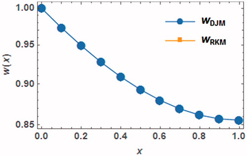
The logarithmic plots of the maximum error remainder parameters, for through are shown in Figure 1 where an exponential rate of convergence can be seen. To show the validity of the DJM; Figure 2 shows the difference between the approximate solution, which is produced by the DJM and the numerical solution that is evaluated by using the RKM (AL-Jawary, 2017).

Figure 1. The logarithmic plots of by DJM when and m=0.3.

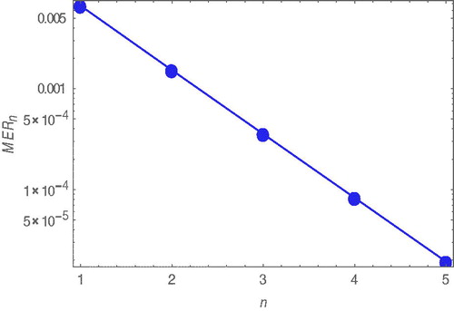
Figure 2. Comparison between the curves of the approximate series function by DJM and the numerical function which obtained by RKM for when and.

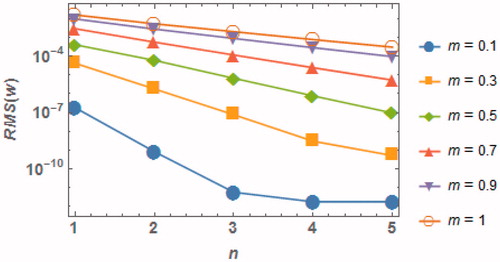
To show the validity for the DJM in reaching the best accuracy for the obtained approximate solutions, we have used the root mean square (RMS) norm to evaluate the difference between the solutions of the DJM and RKM. For this matter, the RMS is given in the following form (35)

Figures 3 and 4 show the RMS differences versus. We observe good convergence in the RMS curves as the value of increases. At constant m note that the higher the value, the larger the RMS difference, as shown in Figure 3. Also, keeping with increasing the values of will make the convergence poorer (Figure 4). In all cases we may conclude that the approximate DJM solution becomes more accurate whenever increases. The rate of convergence with increasing n for the case of β = 0.5 and m = 0.3 was estimated using log(MER₄/MER₃)/log(MER₃/MER₂) = 1.0 proving linear convergence of the method.

Figure 3. The curves of the RMS differences at different values of when

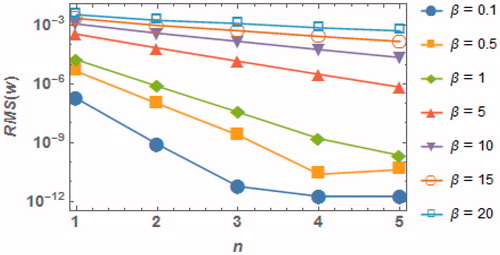
Figure 4. The curves of the RMS differences at different values of when

6. Numerical comparisons

In this section, we present a comparison between our approximate solution obtained using the DJM and the approximate solutions obtained by previous studies using the ADM, VIM-I, VIM-II and VIM-III methods. In comparison, the ADM requires to evaluation the Adomian polynomials, which are computationally expensive. When comparing the DJM with the VIM-; we find that there is no need for evaluating the Lagrange multipliers in DJM, which requires additional calculations when using the VIM-I, VIM-II and VIM-III methods. Furthermore, the final solution in the DJM is based on the sum of resulting iterative terms. In contrast, the VIM-I approximate solution is obtained by taking the limit of the resulting successive approximations. Tables 1 and 2 present the error norm for the solutions obtained by the ADM, VIM- and DJM. It can be clearly seen that the best accuracy is obtained by the DJM numerical solution. The values of the for the fifth order approximate solutions is express smaller error of DJM in comparison to ADM and VIM-I.

Table 1. The for the solutions of the ADM, VIM-I and DJM for different values of when

	ADM	VIM-	DJM
	0.0000512

Table 2. The for the solutions of the ADM, VIM-I and DJM for different values of when

	ADM	VIM-I	DJM

Finally, when comparing the DJM with the other numerical methods, especially Runge–Kutta method (RKM); there is no need to use any type of truncation errors to measure the accuracy of the obtained approximate solution. There is no need for resorting to any discretization processes or determining the step size of the subintervals over the whole interval in the DJM. Furthermore, there is no need for making any round-off errors. The only limitation comes from the physical properties of the underlying problem. As values of the parameters and are increased the nature of the problem changes and thus the error obtained at a specific n increases. Changing of the parameters has an effect on convergence rate as well.

7. Conclusions

In this work, we have derived an approximate solution of the thin film flow of a non-Newtonian fluid by applying the Daftardar-Jafari iterative method. The DJM does not require any restricted assumptions, as they are required when using other iterative methods such as VIM or HAM. Furthermore, there is no need to resort to additional calculations such as evaluating Adomian polynomials as in the case of ADM. The differences and similarities between DJM and VIM were explored in detail, highlighting the most important ones. By examining convergence properties of DJM for several parameter values of the thin film fluid flow problem, we observe good convergence properties. However, we did find that the choice of the parameters does have an effect on convergence.

Acknowledgements

The author would like to thank the anonymous referees, Managing Editor and Editor in Chief for their valuable suggestions.

Disclosure statement

The authors declare that there is no conflict of interest.

References

- Adomian, G. (1994). Solving frontier problems of physics: The decomposition method. Boston, MA: Kluwer Academic Publishers.
- AL-Jawary, M. A. (2016). An efficient iterative method for solving the Fokker–Planck equation. Results in Physics, 6, 985–991. https://doi.org/10.1016/j.rinp.2016.11.018
- AL-Jawary, M. A. (2017). A semi-analytical iterative method for solving nonlinear thin film flow problems. Chaos, Solitons and Fractals, 99, 52–56. https://doi.org/10.1016/j.chaos.2017.03.045
- AL-Jawary, M. A., & AL-Qaissy, H. R. (2015). A reliable iterative method for solving Volterra integro-differential equations and some applications for the Lane–Emden equations of the first kind. Monthly Notices of the Royal Astronomical Society, 448, 3093–3104. doi:10.1093/mnras/stv198
- Al-Jawary, M. A., & Al-Razaq, S. G. (2016). A semi analytical iterative technique for solving duffing equations. International Journal of Pure and Applied Mathematics, 108, 871–885. doi:10.12732/ijpam.v108i4.13
- Al-Jawary, M. A., & Raham, R. K. (2016). A semi-analytical iterative technique for solving chemistry problems. Journal of King Saud University Science, 29, 320–332. https://doi.org/10.1016/j.jksus.2016.08.002
- Banach, S. (1922). Sur les opérations dans les ensembles abstraits et leur application aux equations integrals. Fundamenta Mathematicae, 3, 133–181. https://eudml.org/doc/213289
- Bhalekar, S., & Daftardar-Gejji, V. (2008). New iterative method: Application to partial differential equations. Applied Mathematics and Computation, 203, 778–783. https://doi.org/10.1016/j.amc.2008.05.071
- Bhalekar, S., & Daftardar-Gejji, V. (2011). Convergence of the new iterative method. International Journal of Differential Equations, 2011. doi:10.1155/2011/989065
- Bhalekar, S., & Daftardar-Gejji, V. (2012). Solving a system of nonlinear functional equations using revised new iterative method. Proceedings of World Academy of Science, Engineering and Technology, 68, 08–21. doi:10.1999/1307-6892/1209
- Bhatti, M. M., Zeeshan, A., & Ellahi, R. (2016). Endoscope analysis on peristaltic blood flow of Sisko fluid with Titanium magneto-nanoparticles. Computers in biology and medicine, 78, 29–41. doi:10.1016/j.compbiomed.2016.09.007
- Biazar, J., & Ghazvini, H. (2009). Convergence of the homotopy perturbation method for partial differential equations. Nonlinear Analysis Real World Applications, 10, 2633–2640. https://doi.org/10.1016/j.nonrwa.2008.07.002
- Bildik, N., Konuralp, A., Bek, F., & Kucukarslan, S. (2006). Solution of different type of the partial differential equation by differential transform method and Adomian’s decomposition method. Applied Mathematics and Computation, 172, 551–567. https://doi.org/10.1016/j.amc.2005.02.037
- Daftardar-Gejji, V., & Bhalekar, S. (2010). Solving fractional boundary value problems with Dirichlet boundary conditions using a new iterative method. Computers and Mathematics with Applications, 59, 1801–1809. https://doi.org/10.1016/j.camwa.2009.08.018
- Daftardar-Gejji, V., & Jafari, H. (2006). An iterative method for solving nonlinear functional equations. Journal of Mathematical Analysis and Applications, 316, 753–763. https://doi.org/10.1016/j.jmaa.2005.05.009
- Gul, T., Islam, S., Shah, R. A., Khan, I., & Shafie, S. (2014). Thin film flow in MHD third grade fluid on a vertical belt with temperature dependent viscosity. PLoS One, 9, e97552. doi:10.1371/journal.pone.0097552.
- He, J. H. (1999a). Homotopy perturbation technique. Computer Methods in Applied Mechanics and Engineering, 178, 257–262. https://doi.org/10.1016/S0045-7825(99)00018-3
- He, J. H. (1999b). Variational iteration method-a kind of non-linear analytical technique: some examples. International Journal of Non Linear Mechanics, 34, 699–708. https://doi.org/10.1016/S0020-7462(98)00048-1
- He, J. H. (2000). A coupling method of a homotopy technique and a perturbation technique for non-linear problems. International Journal of Non-Linear Mechanics, 35, 37–43. https://doi.org/10.1016/S0020-7462(98)00085-7
- He, J. H., Wu, G. C., & Austin, F. (2010). The variational iteration method which should be followed. Nonlinear Science Letters A, 1, 1–30. https://works.bepress.com/ji_huan_he/49/
- He, J. H. (2012). Notes on the optimal variational iteration method. Applied Mathematics Letters, 25, 1579–1581. https://doi.org/10.1016/j.aml.2012.01.004
- Hemeda, A. A. (2013). New iterative method: An application for solving fractional physical differential equations. Abstract and Applied Analysis, 2013. http://dx.doi.org/10.1155/2013/617010
- Liao, S. J. (2004). Beyond perturbation: Introduction to homotopy analysis method. Boca Raton: Chapman & Hall/CRC Press.
- Mabood, F. (2014). Comparison of optimal homotopy asymptotic method and homotopy perturbation method for strongly non-linear equation. Journal of the Association of Arab Universities for Basic and Applied Sciences, 16, 21–26. https://doi.org/10.1016/j.jaubas.2013.07.002
- Mabood, F., & Pochai, N. (2015). Comparison of optimal homotopy asymptotic and Adomian decomposition methods for a thin film flow of a third grade fluid on a moving belt. Advances in Mathematical Physics, 2015. doi:10.1155/2015/642835.
- Moosavi, M., Momeni, M., Tavangar, T., Mohammadyari, R., & Rahimi-Esbo, M. (2016). Variational iteration method for flow of non-Newtonian fluid on a moving belt and in a collector. Alexandria Engineering Journal, 55, 1775–1783. https://doi.org/10.1016/j.aej.2016.03.033
- Nemati, H., Ghanbarpour, M., Hajibabayi, M., & Hemmatnezhad. (2009). Thin film flow of non-Newtonian fluids on a vertical moving belt using homotopy analysis method. Journal of Engineering Science and Technology Review, 2, 118–122. https://doaj.org/article/63c97a2d6cb84b3086118e3b1b70b228
- Rajagopal, K. R. (1983). A note on unsteady unidirectional flows of a non-Newtonian fluid. International Journal of Non-Linear Mechanics, 17, 369–373. https://doi.org/10.1016/0020-7462(82)90006-3
- Rashidi, M. M., Bagheri, S., Momoniat, E., & Freidoonimehr, N. (2017). Entropy analysis of convective MHD flow of third grade non-Newtonian fluid over a stretching sheet. Ain Shams Engineering Journal, 8, 77–85. https://doi.org/10.1016/j.asej.2015.08.012
- Ravnik, J., & Skerget, L. (2015). A numerical study of nanofluid natural convection in a cubic enclosure with a circular and an ellipsoidal cylinder. International journal of heat and mass transfer, 89, 596–605. https://doi.org/10.1016/j.ijheatmasstransfer.2015.05.089
- Sajid, M., & Hayat, T. (2008). The application of homotopy analysis method to thin film flows of a third order fluid. Chaos, Solitons and Fractals, 38, 506–515. doi:10.1016/j.chaos.2006.11.034
- Shah, H., Pandya, J., & Shah, P. (2016). Approximate solution for the thin film flow problem of a third grade fluid using spline collocation method. International Journal of Advances in Applied Mathematics and Mechanics, 1, 91–97. https://dx.doi.org/10.22606/jaam.2016.12001
- Sheikholeslami, M., & Zeeshan, A. (2017). Mesoscopic simulation of CuO–H2O nanofluid in a porous enclosure with elliptic heat source. International Journal of Hydrogen Energy, 42, 15393–15402. doi:10.1016/j.ijhydene.2017.04.276
- Siddiqui, A. M., Farooq, A. A., Haroon, T., & Babcock, B. S. (2012a). A comparison of variational iteration and Adomian decomposition methods in solving nonlinear thin film flow problems. Applied Mathematical Sciences, 6, 4911–4919. http://www.m-hikari.com/ams/ams-2012/ams-97-100-2012/babcockAMS97-100-2012-2.pdf
- Siddiqui, A. M., Farooq, A. A., Haroon, T., Rana, M. A., & Babcock, B. S. (2012b). Application of He’s variational iterative method for solving thin film flow problem arising in non-Newtonian fluid mechanics. World Journal of Mechanics, 2, 138–142. doi:10.4236/wjm.2012.23016
- Siddiqui, M., Hameed, M. A., Siddiqui, B. M., & Ghori, Q. K. (2010). Use of Adomian decomposition method in the study of parallel plate flow of a third grade fluid. Communications in Nonlinear Science and Numerical Simulation, 15, 2388–2399. https://doi.org/10.1016/j.cnsns.2009.05.073
- Yaseen, M., Samraiz, M., & Naheed, S. (2013). Exact solutions of Laplace equation by DJ method. Results in physics, 3, 38–40. https://doi.org/10.1016/j.rinp.2013.01.001
- Zeeshan, A., & Atlas, M. (2017). Optimal solution of integro-differential equation of Suspension Bridge Model using Genetic Algorithm and Nelder-Mead method. Journal of the Association of Arab Universities for Basic and Applied Sciences, 24, 310–314. https://doi.org/10.1016/j.jaubas.2017.05.003
- Zeeshan, A., Majeed, A., & Ellahi, R. (2016). Effect of magnetic dipole on radiative non-darcian mixed convective flow over a stretching sheet in porous medium. Journal of Nanofluids, 5, 617–626. doi:10.1166/jon.2016.1237
- Zhou, J. K. (1986). Differential Transformation and its Applications for Electrical Circuits. Wuhan, China: Huazhong Univ. Press. (in Chinese).