A comparative study of analytical solutions of space-time fractional hyperbolic-like equations with two reliable methods

Abstract

This paper deals with a comparative study of analytical solutions of $(n+1)$-dimensional space-time fractional hyperbolic-like equations (with Caputo type fractional derivatives) using two reliable semi-analytical methods: “new integral projected differential transform method (NIPDTM)” and “fractional reduced differential transform method (FRDTM)”. Three test problems are carried out in order to illustrate the efficiency of these methods. The computed results are also compared with the results fromo various schemes, in the literature. The computed series solutions from either method converge to the exact solutions. FRDTM solutions are easy to compute without using any transformation as compared to NIPDTM, but FRDTM needs more iterations to obtain the solutions with the same accuracy.

Keywords:

• New integral transform
• projected differential transform method
• FRDTM
• Caputo fractional derivative
• space- and time fractional hyperbolic-like equations

1. Introduction

Fractional partial differential equations (FPDE) occur more frequently in different research fields. For instance, some of the applications have been identified in image processing, plasma physics, life sciences, electrochemistry, biological modelling, non-linear control theory, and astrophysics etc. (Atangana & Baleanu, 2016; Baleanu, Machado, & Luo, 2012; Carpinteri & Mainardi, 1997; El-Sayed, 1996; He, 1998, 1999; Herzallah, El-Sayed, & Baleanu, 2010; Jesus & Machado, 2008; Magin, 2006; Mainardi, 1971; Miller & Ross, 1993; Tarasov, 2008). In FPDEs, many models are associated with ecology, water waves, vibrations of strings or membranes, propagation of sound waves and electromagnetic waves or transmissions of electric signals in cables are generally described as wave equations. Space and time fractional wave and heat equations appear mainly in conventional diffusion or wave equations, with fractional derivative of arbitrary order instead of conventional derivative (Mainardi, 1971). These space-time fractional wave equations have many applications such as: to investigate Brownian diffusion, unification of diffusion and propagation phenomena of a wave, sub-diffusion systems, and random walk (Agrawal, 2002; Andrezei, 2002; Klafter, Blumen, & Zumofen, 1984).

We consider multi-dimensional space-time fractional hyperbolic-like equation of the form (1) $$\begin{array}{c}{\mathcal{D}}_t^{\alpha }u(X,t)=f_1\left(X\right){\mathcal{D}}_{x_1}^{\beta }u(X,t)+f_2\left(X\right){\mathcal{D}}_{x_2}^{\beta }u(X,t)\hfill \\ +\dots +f_n\left(X\right){\mathcal{D}}_{x_n}^{\beta }u(X,t)+h(X,t),\hfill \\ u(X,0)={\psi }_0\left(X\right),{\frac{\partial u(X,t)}{\partial t}|}_{t=0}={\psi }_1\left(X\right),\hspace{0.5em}1<\alpha , \beta \le 2,\hfill \end{array}$$(1) where $D_t^{\alpha }u=\frac{{\partial }^{\alpha }u}{\partial t^{\alpha }}$ represents Caputo fractional derivative of u, u(X, t) is the density of the diffusing material at point $X=(x_1,\dots ,x_n)$ at time t, and $f_1,\dots ,f_n$ are the diffusion coefficients for u at X, h is a smooth function. If $h=0,$ diffusion coefficients are independent of the density (i.e. $f_1=f_2=\dots =f_n={\sigma }^2$, a constant) and β = 2, then Eq. (1)(1) $$\begin{array}{c}{\mathcal{D}}_t^{\alpha }u(X,t)=f_1\left(X\right){\mathcal{D}}_{x_1}^{\beta }u(X,t)+f_2\left(X\right){\mathcal{D}}_{x_2}^{\beta }u(X,t)\hfill \\ +\dots +f_n\left(X\right){\mathcal{D}}_{x_n}^{\beta }u(X,t)+h(X,t),\hfill \\ u(X,0)={\psi }_0\left(X\right),{\frac{\partial u(X,t)}{\partial t}|}_{t=0}={\psi }_1\left(X\right),\hspace{0.5em}1<\alpha , \beta \le 2,\hfill \end{array}$$(1) reduces to time-fractional wave equation, i.e. $D_t^{\alpha }u={\sigma }^2{\nabla }^{2}u$, and for constant diffusion coefficient, Eq. (1)(1) $$\begin{array}{c}{\mathcal{D}}_t^{\alpha }u(X,t)=f_1\left(X\right){\mathcal{D}}_{x_1}^{\beta }u(X,t)+f_2\left(X\right){\mathcal{D}}_{x_2}^{\beta }u(X,t)\hfill \\ +\dots +f_n\left(X\right){\mathcal{D}}_{x_n}^{\beta }u(X,t)+h(X,t),\hfill \\ u(X,0)={\psi }_0\left(X\right),{\frac{\partial u(X,t)}{\partial t}|}_{t=0}={\psi }_1\left(X\right),\hspace{0.5em}1<\alpha , \beta \le 2,\hfill \end{array}$$(1) reduces to classical wave equation $u_{tt}={\sigma }^2{\nabla }^{2}u$ when α = 2). The fundamental solution in 1 D was computed first in (Mainardi, 1996), later in (Hanyga, 2002) for a multi-dimensional case, and in a simpler form (Mentrelli & Pagnini, 2015). The hyperbolic-like model describes many physical problems in different fields of science and engineering such as earthquake stresses (Holliday, Rundle, Tiampo, Klein, & Donnellan, 2006) and non-homogeneous elastic waves in soils (Manolis & Rangelov, 2006).

In recent years, a great deal of effort has been expanded to develop techniques for the computation of the approximate solution behavior of the fractional differential equations, see (Singh & Kumar, 2018, 2017a, 2016) and the references therein. Fu et al. studied numerically the space-fractional parabolic-like models by implementing the Kansa method (Pang, Chen, & Fu, 2015), the time-fractional parabolic-like models by implementing the Boundary particle method (Fu, Chen, & Yang, 2013) while constant- and variable-order time-fractional parabolic-like models were studied by implementing a domain-type meshless method (Fu, Chen, & Ling, 2015). Time-fractional parabolic-like and hyperbolic-like models have been studied by using many techniques, among them the homotopy perturbation Sumudu transform method (Singh, Kumar, & Kilicman, 2013), the adomian decomposition method (Momani, 2005; Wazwaz & Goruis, 2004), the variational iteration method (Shou & He, 2008), the homotopy perturbation method (Özis & Agirseven, 2008), the reduced differential transforms method (Arshad, Lu, & Wang, 2017; Singh & Srivastava, 2015; Taghizadeh & Noori, 2017) while fractional parabolic-like (or hyperbolic-like) equations have been studied using the differential transforms method (Secer, 2012), the modified homotopy perturbation method (Jafari & Momani, 2007), the homotopy analysis method (Xu & Cang, 2008; Zhang, Zhao, Liu, & Tang, 2014), the variational iteration method (Molliq, Noorani, & Hashim, 2009; Yin, Song, & Cao, 2013), the modified homotopy analysis method (Yin, Kumar, & Kumar, 2015), the fractional homotopy analysis transforms method (Khader, Kumar, & Abbasbandy, 2016), the fractional variational iteration method with He’s polynomials (Tang, Wang, Wei, & Zhang, 2014), the homotopy decomposition method (HDM) (Atangana & Alabaraoye, 2013), the homotopy analysis fractional Sumudu transforms method (Pandey and Mishra, 2017), and the variable separation method (Zhang, Zhu, & Zhang, 2016).

In present paper my main goal is to compute approximate series solutions of (n + 1)D space-time fractional hyperbolic (STFH)-like equation with appropriate initial conditions using FRDTM (Arshad et al., 2017; Singh & Srivastava, 2015) and NIPDTM (Kunjan, Twinkle, & Kilicman, 2017).

2. Basic definitions and notations

The definitions of Caputo order fractional integration and differentiation and its properties as in (Miller & Ross, 1993; Singh and Kumar, 2018, 2017a) which are used throughout the paper are listed below:

((Miller & Ross, 1993)) Let $\mu \in \mathbb{R}$ and $m\in \mathbb{N}$. A function $f:{\mathbb{R}}^{+}\to \mathbb{R}$ belongs to ${\mathbb{C}}_{\mu }$ if there exists $k\in \mathbb{R},k>\mu$ and $g\in C[0,\infty )$ such that $f(x)=x^{k}g(x),\forall x\in {\mathbb{R}}^{+}$. Moreover, $f\in {\mathbb{C}}_{\mu }^m$ if $f^{(m)}\in {\mathbb{C}}_{\mu }$.

((Miller & Ross, 1993; Singh and Kumar, 2017a)) Let $f\in {\mathbb{C}}_{\mu }$, then R-L fractional derivative, ${\mathcal{J}}_t^{\alpha }(f)$ ($\alpha \ge 0$), of f is defined by ${\mathcal{J}}_t^{0}f(t)=f(t)$ and $${\mathcal{J}}_t^{\alpha }f\left(t\right)=\frac{1}{\Gamma (\alpha )}\underset{0}{\overset{\mathrm{t}}{\int }}{\left(\mathrm{t}-\tau \right)}^{\alpha -1}f(\tau )\mathrm{d}\tau , \text{if} \alpha >0, \text{where} \Gamma \left(z\right):=\underset{0}{\overset{\infty }{\int }}{e}^{-t}{t}^{z-1}dt.$$

((Miller & Ross, 1993; Singh and Kumar, 2017a)) Let $f\in {\mathbb{C}}_{\mu },\mu \ge -1$ and $m-1<\alpha \le m,m\in \mathbb{N}$. Then ${\mathcal{D}}_t^{\alpha }f(t)={\mathcal{J}}_t^{m-\alpha }{\mathcal{D}}_t^{m}f(t)$.

Some basic properties of the operator ${\mathcal{D}}_t^{\alpha }$ are as follows:

Let $m-1<\alpha \le m\in \mathbb{N},f\in {\mathbb{C}}_{\mu }^m,\mu \ge -1,\gamma >\alpha -1$, then for t > 0 and for a constant C (2) $$\begin{array}{c}\left(a\right) {\mathcal{D}}_t^{\alpha }{\mathcal{J}}_t^{\alpha }f\left(t\right)=f\left(t\right); \left(b\right) {\mathcal{D}}_t^{\alpha }{t}^{\gamma }=\frac{\Gamma (1+\gamma )}{\Gamma (1+\gamma -\alpha )}{t}^{\gamma -\alpha };\left(c\right) {\mathcal{D}}_t^{\alpha }C=0;\hfill \\ \left(d\right) {\mathcal{J}}_t^{\alpha }{\mathcal{D}}_t^{\alpha }f\left(t\right)=f\left(t\right)-\sum _{k=0}^m{f}^{\left(k\right)}\left(0^{+}\right)\frac{t^k}{k!}.\hfill \end{array}$$(2)

The Caputo fractional derivative deals with traditional initial and boundary conditions in the formulation of the physical problems, see (Atangana & Baleanu, 2016; Baleanu et al., 2012; Carpinteri & Mainardi, 1997; Mainardi, 1971; Miller & Ross, 1993).

2.1. Fractional reduced differential transform method

This section describes the basic properties of FRDTM (Arshad et al., 2017; Singh & Srivastava, 2015; Singh & Kumar, 2017).

Using the basic properties of 1-dim DTM, a function ψ of two variables with the separation property $\psi (x,t)=f(x)g(t)$ can be embodied as (3) $$\psi \left(x,t\right)=\sum _{\ell =0}^{\infty }{F}_{\alpha }\left(\ell \right)t^{\alpha \ell }\sum _{j=0}^{\infty }G\left(j\right)x^j=\sum _{\ell =0}^{\infty }{\Psi }_{\alpha }^{\ell }\left(x\right)t^{\alpha \ell },$$(3)

where $0<\alpha \le 1,{\Psi }_{\alpha }^{\ell }(x):=G(j)F_{\alpha }(\ell )x^j$ is the spectrum of $\psi (x,t)$. Throughout the paper ${\Psi }_{\alpha }^{\ell }(x)$ (uppercase) is used for FRDT of function $\psi (x,t)$ (lowercase). Some basic properties of FRDTM are described in the following:

((Arshad et al., 2017; Singh & Srivastava, 2015; Singh & Kumar, 2017)) Let $\psi (x,t)$ be an analytic and continuously differentiable, then (a) FRDT or the spectrum of ψ is given by $${\Psi }_{\alpha }^k(x)=\frac{1}{\Gamma (k\alpha +1)}{\left[{\mathcal{D}}_t^{\alpha k}(\psi (x,t))\right]}_{t=t_0},\hspace{1em}k=0,1,2,\dots$$where ${\mathcal{D}}_t^{\alpha k}\equiv \frac{{\partial }^{\alpha k}}{\partial t^{\alpha k}}$, α describes the order of time-fractional derivative.(b) The inverse FRDT of ${\Psi }_{\alpha }^k(x)$ is defined by $$\psi \left(x,t\right)=\underset{m\to \infty }{\lim }{s}_m=\sum _{k=0}^{\infty }{\Psi }_{\alpha }^k\left(x\right){\left(t-t_0\right)}^{k\alpha }.$$

where $s_m={\sum }_{k=0}^m{\Psi }_{\alpha }^k(x){(t-t_0)}^{k\alpha }$ denotes the mth order approximate solution.

In particular for $t_0=0$ , we get $\psi \left(x,t\right)=\sum _{k=0}^{\infty }{\Psi }_{\alpha }^k\left(x\right)t^{k\alpha }.$

Let $X=(x_1,x_2,\dots ,x_n)$ be a vector of n variables. Some basis properties of FRDTM are listed below

Theorem 2.6.

((Arshad et al., 2017; Singh & Kumar, 2017)) Let ${\Psi }_{\alpha }^k(X)$ and ${\Phi }_{\alpha }^k(X)$ be the spectrums of the analytic and continuously differentiable functions $\psi (X,t)$ and $\varphi (X,t)$, respectively, and

1. If $\theta (X,t)={\ell }_1\psi (X,t)\pm {\ell }_2\varphi (X,t)$, then $${\Theta }_{\alpha }^k\left(X\right)={\ell }_1{\Psi }_{\alpha }^k\left(X\right)\pm {\ell }_2{\Phi }_{\alpha }^k\left(X\right).$$

2. If $\theta (X,t)=\psi (X,t)\varphi (X,t)$, then ${\Theta }_{\alpha }^k(X)={\sum }_{r=0}^k{\Psi }_{\alpha }^r(X){\Psi }_{\alpha }^{k-r}(X).$

3. If $\theta (x,t)=f(X)\psi (X,t)$, then $${\Theta }_{\alpha }^k\left(X\right)=f\left(X\right){\Psi }_{\alpha }^k\left(X\right).$$

4. If $\theta (X,t)=x_i^m{t}^n\psi (X,t)$, then ${\Theta }_{\alpha }^k(X)=\{\begin{array}{cc}{x}_i^m{\Psi }_{\alpha }^{k\alpha -n}(X)\hfill & if k\alpha \ge n\hfill \\ 0,\hfill & \mathit{\text{else}}.\hfill \end{array}$

5. If $\theta (X,t)={\mathcal{D}}_{x_i}^{\beta }\psi (X,t)$; $\varphi (X,t)=x_i^m{t}^{\gamma }$. Then $${\Theta }_{\alpha }^k\left(X\right)={\mathcal{D}}_{x_i}^{\beta }{\Psi }_{\alpha }^k\left(X\right);\hspace{1em}\hspace{1em}{\Phi }_{\alpha }^k\left(X\right)=x_i^m\delta (k\alpha -\gamma );\delta \left(k\right)=\{\begin{array}{cc}1\hfill & if k=0\hfill \\ 0\hfill & \mathit{\text{otherwise}}\hfill \end{array}$$

6. If $\theta (X,t)=D_{x_i}^{r_i}{D}_t^{n\alpha }\psi (X,t)$. Then ${\Theta }_{\alpha }^k(X)=\frac{\Gamma (1+(k+n)\alpha )}{\Gamma (1+k\alpha )}{D}_{x_i}^{r_i}{\Psi }_{\alpha }^k(X).$ In particular,

   1. If $\theta (X,t)=D_{x_i}^{r_i}\psi (X,t)$. Then ${\Theta }_{\alpha }^k(X)=D_{x_i}^{r_i}{\Psi }_{\alpha }^k(X).$

   2. If $\theta (X,t)=D_t^{n\alpha }\psi (X,t)$. Then ${\Theta }_{\alpha }^k(X)=\frac{\Gamma (1+(k+n)\alpha )}{\Gamma (1+k\alpha )}{\Psi }_{\alpha }^k(X).$

7. If $\theta (X)={\frac{{\partial }^{\beta }\psi (X,t)}{\partial t^{\beta }}|}_{t=0}$, then $${\Theta }_{\alpha }^r\left(X\right)=\{\begin{array}{cc}{\Psi }_{\alpha }^r\left(X\right)\hfill & if r\alpha =m\hfill \\ 0\hfill & \mathit{\text{otherwise}}\hfill \end{array},r=0,1,\dots \frac{\beta }{\alpha }-1.$$

For more details we refer the readers to (Arshad et al., 2017; Singh & Kumar, 2017).

2.2. New integral projected differential transform method (NIPDTM)

Let $\mathcal{F}$ be the set of functions of exponential order as defined below: (4) $$\mathcal{F}=\{f\left(t\right):\exists M,k_1,k_2>0 \text{such that} \left|f\right(t\left)\right|\le M{e}^{\frac{\left|t\right|}{k_i^2}} \text{whenever} t\in {(-1)}^i\times [0,\infty )\},$$(4) where a given $f\in \mathcal{F}$ the constant M must be finite while k₁, k₂ may be finite or infinite.

Definition 2.7.

The new integral transform $\mathcal{K}\left\{u(t)\right\}=\mathcal{U}(\mu )$ of $u(t)\in \mathcal{F}$ is defined by (5) $$\mathcal{U}(\mu )=\mathcal{K}\left\{u\left(t\right)\right\}=\frac{1}{\mu }{\int }_0^{\infty }{e}^{\frac{-t}{{\mu }^2}}u\left(t\right)dt$$(5)

The following are some properties of new integral transform

Theorem 2.8.

((Kunjan et al., 2017)) $a)$ The new integral transform of $\frac{{\partial }^{n}u}{\partial t^n}$ is given by (6) $$\mathcal{K}\left\{\frac{{\partial }^{n}u(x,t)}{\partial t^n}\right\}=\frac{\mathcal{U}(x,\mu )}{{\mu }^{2n}}-\sum _{k=0}^{n-1}\frac{1}{{\mu }^{2(n-k)-1}}\frac{{\partial }^{k}u(x,0^{+})}{\partial t^k},n\ge 1.$$(6)

$b)$ The new integral transform of the Caputo fractional derivative $D_t^{\alpha }u(x,t)$ and Riemann-Liouville fractional integral ${\mathcal{J}}_t^{\alpha }u(x,t)$ of u(x, t) is given by

1. $\mathcal{K}\left\{{\mathcal{J}}_t^{\alpha }u(x,t)\right\}={\mu }^{2\alpha }\mathcal{U}(x,\mu ),$

2. $\mathcal{K}\{{\mathcal{D}}_t^{\alpha }u(x,t)\}=\frac{\mathcal{U}(x,\mu )}{{\mu }^{2\alpha }}-{\sum }_{k=0}^{n-1}\frac{1}{{\mu }^{2(\alpha -k)-1}}\frac{{\partial }^{k}u(x,0^{+})}{\partial t^k},n-1<\alpha \le n\in \mathbb{N},$ $$c)\mathcal{K}\left\{\frac{t^{n\alpha }}{\Gamma (1+n\alpha )}\right\}={\mu }^{2n\alpha +1}.$$

For more details on the properties of new integral transform, we refer the readers to (Kashuri & Fundo, 2013; Kashuri, Fundo, & Kreku, 2013).

2.2.1. Implementation of NIPDTM on fractional hyperbolic-like equations

The new integral transform on Eq. (1)(1) $$\begin{array}{c}{\mathcal{D}}_t^{\alpha }u(X,t)=f_1\left(X\right){\mathcal{D}}_{x_1}^{\beta }u(X,t)+f_2\left(X\right){\mathcal{D}}_{x_2}^{\beta }u(X,t)\hfill \\ +\dots +f_n\left(X\right){\mathcal{D}}_{x_n}^{\beta }u(X,t)+h(X,t),\hfill \\ u(X,0)={\psi }_0\left(X\right),{\frac{\partial u(X,t)}{\partial t}|}_{t=0}={\psi }_1\left(X\right),\hspace{0.5em}1<\alpha , \beta \le 2,\hfill \end{array}$$(1) with Theorem 2.8(a) yields (7) $$\begin{array}{c}\mathcal{U}(X,\mu )=\mu {\psi }_0\left(X\right)+{\mu }^3{\psi }_1\left(X\right)+{\mu }^{2\alpha }\mathcal{H}(X,\mu )+{\mu }^{2\alpha }\mathcal{K}\{f_1\left(X\right){\mathcal{D}}_{x_1}^{\beta }u(X,t)+f_2\left(X\right){\mathcal{D}}_{x_2}^{\beta }u(X,t)+\dots +f_n\left(X\right){\mathcal{D}}_{x_n}^{\beta }u(X,t)\}.\hfill \end{array}$$(7)

Inverse new integral transform on (7) yields (8) $$\begin{array}{c}u(X,t)={\psi }_0\left(X\right)+t{\psi }_1\left(X\right)+{\mathcal{K}}^{-1}\left\{{\mu }^{2\alpha }\mathcal{H}(X,\mu )\right\}+{\mathcal{K}}^{-1}\{{\mu }^{2\alpha }\mathcal{K}\{f_1\left(X\right)\times {\mathcal{D}}_{x_1}^{\beta }u(X,t)+f_2\left(X\right){\mathcal{D}}_{x_2}^{\beta }u(X,t)+\dots +f_n\left(X\right){\mathcal{D}}_{x_n}^{\beta }u(X,t)\}\}\hfill \end{array}$$(8)

The projected differential transform (PDT) on (8) yields (9) $$\{\begin{array}{c}U(X,0)=g_1(X,t,),\hfill \\ U(X,\ell +1)={\mathcal{K}}^{-1}\{{\mu }^{2\alpha }\mathcal{K}\{f_1\left(X\right){\mathcal{D}}_{x_1}^{\beta }U(X,\ell )\hfill \\ +f_2\left(X\right){\mathcal{D}}_{x_2}^{\beta }U(X,\ell )\hfill \\ +\dots +f_n\left(X\right){\mathcal{D}}_{x_n}^{\beta }U(X,\ell )\}\},\ell \ge 0.\hfill \end{array}$$(9)

where $g_1(X,t)={\psi }_0(X)+t{\psi }_1(X)+{\mathcal{K}}^{-1}\left\{{\mu }^{2\alpha }\mathcal{H}(X,\mu )\right\}$.

The expression (9) is referred to as” new integral-projected differential transform (NIPDT)” of problem (1). The mth order series solution of Eq. (1)(1) $$\begin{array}{c}{\mathcal{D}}_t^{\alpha }u(X,t)=f_1\left(X\right){\mathcal{D}}_{x_1}^{\beta }u(X,t)+f_2\left(X\right){\mathcal{D}}_{x_2}^{\beta }u(X,t)\hfill \\ +\dots +f_n\left(X\right){\mathcal{D}}_{x_n}^{\beta }u(X,t)+h(X,t),\hfill \\ u(X,0)={\psi }_0\left(X\right),{\frac{\partial u(X,t)}{\partial t}|}_{t=0}={\psi }_1\left(X\right),\hspace{0.5em}1<\alpha , \beta \le 2,\hfill \end{array}$$(1) is given by (10) $$s_m=\sum _{\ell =0}^{m}U(X,\ell ),$$(10)

and so, the series solution of Eq. (1)(1) $$\begin{array}{c}{\mathcal{D}}_t^{\alpha }u(X,t)=f_1\left(X\right){\mathcal{D}}_{x_1}^{\beta }u(X,t)+f_2\left(X\right){\mathcal{D}}_{x_2}^{\beta }u(X,t)\hfill \\ +\dots +f_n\left(X\right){\mathcal{D}}_{x_n}^{\beta }u(X,t)+h(X,t),\hfill \\ u(X,0)={\psi }_0\left(X\right),{\frac{\partial u(X,t)}{\partial t}|}_{t=0}={\psi }_1\left(X\right),\hspace{0.5em}1<\alpha , \beta \le 2,\hfill \end{array}$$(1) is given by (11) $$u(X,t)=\underset{m\to \infty }{\lim }{s}_m.$$(11)

3. Solutions of $(n+1)$D STFH-like equation via FRDTM and NIPDTM

This section deals with the main goal of the paper, to present numerical study of three test problems of $(n+1)$D STFH-like diffusion equations using FRDTM and NIPDTM to validate their reliability and efficiency.

Example 3.1.

Consider initial values system of $(1+1)$D STFH-like equation (12) $$\begin{array}{c}{\mathcal{D}}_t^{\alpha }u(x,t)=\frac{x^2}{2}\frac{{\partial }^{\beta }u(x,t)}{\partial x^{\beta }}, u(x,0)=x, \frac{\partial u(x,0)}{\partial t}=x^2, 1<\alpha ,\beta \le 2\hfill \end{array}$$(12)

(a) NIPDTM: The NIPDT on Eq. (12)(12) $$\begin{array}{c}{\mathcal{D}}_t^{\alpha }u(x,t)=\frac{x^2}{2}\frac{{\partial }^{\beta }u(x,t)}{\partial x^{\beta }}, u(x,0)=x, \frac{\partial u(x,0)}{\partial t}=x^2, 1<\alpha ,\beta \le 2\hfill \end{array}$$(12) yields (13) $$\begin{array}{c} U(x,\ell +1)={\mathcal{K}}^{-1}\left\{{\mu }^{2\alpha }\mathcal{K}\left\{\frac{x^2}{2}\frac{{\partial }^{\beta }U(x,\ell )}{\partial x^{\beta }}\right\}\right\},\ell \ge 0;\hspace{1em}U(x,0)=x+t{x}^2.\hfill \end{array}$$(13)

The solution of the relation (13) is obtained as follows: $$\begin{array}{c}U(x,0)=x+t{x}^2, U(x,1)=\frac{x^{4-\beta }}{\Gamma (3-\beta )}\frac{t^{\alpha +1}}{\Gamma (2+\alpha )},U(x,2)=\frac{\Gamma (5-\beta )x^{6-2\beta }}{2\Gamma (3-\beta )\Gamma (5-2\beta )}\frac{t^{2\alpha +1}}{\Gamma (2+2\alpha )},\hfill \\ U(x,3)=\frac{\Gamma (5-\beta )\Gamma (7-2\beta )x^{8-3\beta }}{4\Gamma (3-\beta )\Gamma (5-2\beta )\Gamma (7-3\beta )}\frac{t^{3\alpha +1}}{\Gamma (2+3\alpha )},\hfill \\ U(x,4)=\frac{\Gamma (5-\beta )\Gamma (7-2\beta )\Gamma (9-3\beta )x^{10-4\beta }}{8\Gamma (3-\beta )\Gamma (5-2\beta )\Gamma (7-3\beta )\Gamma (9-4\beta )}\frac{t^{4\alpha +1}}{\Gamma (2+4\alpha )},\hfill \\ U(x,5)=\frac{\Gamma (5-\beta )\Gamma (7-2\beta )\Gamma (9-3\beta )\Gamma (11-4\beta )x^{12-5\beta }}{16\Gamma (3-\beta )\Gamma (5-2\beta )\Gamma (7-3\beta )\Gamma (9-4\beta )\Gamma (11-5\beta )}\frac{t^{5\alpha +1}}{\Gamma (2+5\alpha )},\dots \hfill \end{array}$$

Thus, the solution of the problem (12), (14) $$\begin{array}{c}u(x,t)=\sum _{\ell =0}^{\infty }U(x,\ell )=x+t{x}^2+\frac{x^{4-\beta }}{\Gamma (3-\beta )}\frac{t^{\alpha +1}}{\Gamma (2+\alpha )}+\frac{\Gamma (5-\beta )x^{6-2\beta }}{2\Gamma (3-\beta )\Gamma (5-2\beta )}\frac{t^{2\alpha +1}}{\Gamma (2+2\alpha )}\hfill \\ +\frac{\Gamma (5-\beta )\Gamma (7-2\beta )x^{8-3\beta }}{4\Gamma (3-\beta )\Gamma (5-2\beta )\Gamma (7-3\beta )}\frac{t^{3\alpha +1}}{\Gamma (2+3\alpha )}+\frac{\Gamma (5-\beta )\Gamma (7-2\beta )\Gamma (9-3\beta )x^{10-4\beta }}{8\Gamma (3-\beta )\Gamma (5-2\beta )\Gamma (7-3\beta )\Gamma (9-4\beta )}\frac{t^{4\alpha +1}}{\Gamma (2+4\alpha )}\hfill \\ +\frac{\Gamma (5-\beta )\Gamma (7-2\beta )\Gamma (9-3\beta )\Gamma (11-4\beta )x^{12-5\beta }}{16\Gamma (3-\beta )\Gamma (5-2\beta )\Gamma (7-3\beta )\Gamma (9-4\beta )\Gamma (11-5\beta )}\frac{t^{5\alpha +1}}{\Gamma (2+5\alpha )}+\dots \hfill \end{array}$$(14)

In particular for $\beta \to 2$, solution (14) reduces to (15) $$u(x,t)=x+x^2\left\{t+\frac{t^{\alpha +1}}{\Gamma (2+\alpha )}+\frac{t^{2\alpha +1}}{\Gamma (2+2\alpha )}+\frac{t^{3\alpha +1}}{\Gamma (2+3\alpha )}+\dots \right\}=x+x^{2}t{E}_{\alpha ,2}\left(t^{\alpha }\right)$$(15)

where $E_{\sigma ,\delta }(t)={\sum }_{n=0}^{\infty }\frac{t^n}{\Gamma (\sigma n+\delta )}$ for $\sigma ,\delta \ge 0$ is referred to as Mittag-Leffler function with two parameters (Carpinteri & Mainardi, 1997; Mainardi, 1971). It is worth to note that solution (15) is the same as the analytical solution obtained by using DTM (Secer, 2012), ADM (Momani, 2005), modified HPM (Jafari & Momani, 2007), VIM (Yin et al., 2013), modified HAM (Yin et al., 2015) and FHATM (Khader et al., 2016). For $\alpha =2,\beta =2$, we get (16) $$u(x,t)=x+x^2\left(t+\frac{t^3}{6}+\frac{t^5}{120}+\dots \right)=x+x^2\sinh \left(t\right)$$(16)

Eq. (16)(16) $$u(x,t)=x+x^2\left(t+\frac{t^3}{6}+\frac{t^5}{120}+\dots \right)=x+x^2\sinh \left(t\right)$$(16) is solution of associated classical hyperbolic wave equation, which is same as obtained in (Momani, 2005; Taghizadeh & Noori, 2017). Hence, the computed results approach towards the exact results and are in good agreement with the results due to earlier schemes.

(b) FRDTM: For $\alpha =N\eta$, the FRDTM of (12) yields (17) $$\{\begin{array}{c}{U}_{\eta }^0\left(x\right)=x, \text{and} U_{\eta }^r\left(x\right)=\{\begin{array}{cc}{x}^2,\hfill & \text{if} r\eta =1,\hfill \\ 0,\hfill & \text{if} r\eta \ne 1,\hfill \end{array} r\in \{1,\dots N-1\}\hfill \\ U_{\eta }^{k+N}\left(x\right)=\frac{\Gamma (k\eta +1)}{\Gamma \left(\right(k+N)\eta +1)}\frac{x^2}{2}\frac{{\partial }^{\beta }{U}_{\eta }^k\left(x\right)}{\partial x^{\beta }},k\ge 0.\hfill \end{array}$$(17)

It is worth mentioning that the recurrence relation (17) can be solved for any given α, which confirms that FRDTM solution can be obtained for any given alpha. But a general solution in terms of arbitrary value of alpha cannot be obtained. More precisely, for any two different values of α one has to solve the recurrence relation (17), separately.

(i) If $\alpha =1.5$ (i.e., $\eta =\frac{1}{2}$, N = 3): Then the recursive values of $U_{\frac{1}{2}}^k(x)$’s are obtained from (17) as follows: $$\begin{array}{c}{U}_{\frac{1}{2}}^0\left(x\right)=x, U_{\frac{1}{2}}^1\left(x\right)=0, U_{\frac{1}{2}}^2\left(x\right)=x^2, U_{\frac{1}{2}}^3\left(x\right)=0, U_{\frac{1}{2}}^4\left(x\right)=0, U_{\frac{1}{2}}^5\left(x\right)=\frac{x^{4-\beta }}{\Gamma (3-\beta )\Gamma \left(\frac{7}{2}\right)},\hfill \\ U_{\frac{1}{2}}^6\left(x\right)=0, U_{\frac{1}{2}}^7\left(x\right)=0, U_{\frac{1}{2}}^8\left(x\right)=\frac{\Gamma (5-\beta )x^{6-2\beta }}{2\Gamma \left(5\right)\Gamma (3-\beta )\Gamma (5-2\beta )},\hfill \\ U_{\frac{1}{2}}^9\left(x\right)=0, U_{\frac{1}{2}}^{10}\left(x\right)=0, U_{\frac{1}{2}}^{11}\left(x\right)=\frac{\Gamma (5-\beta )\Gamma (7-2\beta )x^{8-3\beta }}{4\Gamma \left(\frac{13}{2}\right)\Gamma (3-\beta )\Gamma (5-2\beta )\Gamma (7-3\beta )},\hfill \\ U_{\frac{1}{2}}^{12}\left(x\right)=0, U_{\frac{1}{2}}^{13}\left(x\right)=0, U_{\frac{1}{2}}^{14}\left(x\right)=\frac{\Gamma (5-\beta )\Gamma (7-2\beta )\Gamma (9-3\beta )x^{10-4\beta }}{8\Gamma \left(8\right)\Gamma (3-\beta )\Gamma (5-2\beta )\Gamma (7-3\beta )\Gamma (9-4\beta )},\hfill \\ U_{\frac{1}{2}}^{15}\left(x\right)=0, U_{\frac{1}{2}}^{16}\left(x\right)=0, U_{\frac{1}{2}}^{17}\left(x\right)=\frac{\Gamma (5-\beta )\Gamma (7-2\beta )\Gamma (9-3\beta )\Gamma (11-4\beta )x^{12-5\beta }}{16\Gamma \left(\frac{19}{2}\right)\Gamma (3-\beta )\Gamma (5-2\beta )\Gamma (7-3\beta )\Gamma (9-4\beta )\Gamma (11-5\beta )},\dots \hfill \end{array}$$

Thus, inverse FRDTM leads the solution of the problem (12) as follows: (18) $$\begin{array}{c}u(x,t)=\sum _{\ell =0}^{\infty }{U}_{\eta }^{\ell }\left(x\right)t^{\ell \eta }=x+t{x}^2+\frac{x^{4-\beta }{t}^{\frac{5}{2}}}{\Gamma (3-\beta )\Gamma \left(\frac{7}{2}\right)}\hfill \\ +\frac{\Gamma (5-\beta )x^{6-2\beta }{t}^4}{2\Gamma \left(5\right)\Gamma (3-\beta )\Gamma (5-2\beta )}+\frac{\Gamma (5-\beta )\Gamma (7-2\beta )x^{8-3\beta }{t}^{\frac{11}{2}}}{4\Gamma \left(\frac{13}{2}\right)\Gamma (3-\beta )\Gamma (5-2\beta )\Gamma (7-3\beta )}\hfill \\ +\frac{\Gamma (5-\beta )\Gamma (7-2\beta )\Gamma (9-3\beta )x^{10-4\beta }{t}^7}{8\Gamma \left(8\right)\Gamma (3-\beta )\Gamma (5-2\beta )\Gamma (7-3\beta )\Gamma (9-4\beta )}\hfill \\ +\frac{\Gamma (5-\beta )\Gamma (7-2\beta )\Gamma (9-3\beta )\Gamma (11-4\beta )x^{12-5\beta }{t}^{\frac{17}{2}}}{16\Gamma \left(\frac{19}{2}\right)\Gamma (3-\beta )\Gamma (5-2\beta )\Gamma (7-3\beta )\Gamma (9-4\beta )\Gamma (11-5\beta )}+\dots \hfill \end{array}$$(18)

(ii) If $\alpha =1.75$ (i.e., $\eta =\frac{1}{4}$, N = 7): Similar to case (i), recursive values of $U_{\frac{1}{4}}^k(x)$’s can be obtained direct from (17), and so, inverse FRDTM leads the solution of the problem (12) for $\eta =\frac{1}{4}$ as follows: (19) $$\begin{array}{c}u(x,t)=\sum _{\ell =0}^{\infty }{U}_{\frac{1}{4}}^{\ell }\left(x\right)t^{\frac{\ell }{4}}=x+t{x}^2+\frac{x^{4-\beta }{t}^{\frac{11}{4}}}{\Gamma (3-\beta )\Gamma \left(\frac{15}{4}\right)}\hfill \\ +\frac{\Gamma (5-\beta )x^{6-2\beta }{t}^{\frac{18}{4}}}{2\Gamma \left(\frac{22}{4}\right)\Gamma (3-\beta )\Gamma (5-2\beta )}+\frac{\Gamma (5-\beta )\Gamma (7-2\beta )x^{8-3\beta }{t}^{\frac{25}{4}}}{4\Gamma \left(\frac{29}{4}\right)\Gamma (3-\beta )\Gamma (5-2\beta )\Gamma (7-3\beta )}\hfill \\ +\frac{\Gamma (5-\beta )\Gamma (7-2\beta )\Gamma (9-3\beta )x^{10-4\beta }{t}^8}{8\Gamma \left(9\right)\Gamma (3-\beta )\Gamma (5-2\beta )\Gamma (7-3\beta )\Gamma (9-4\beta )}\hfill \\ +\frac{\Gamma (5-\beta )\Gamma (7-2\beta )\Gamma (9-3\beta )\Gamma (11-4\beta )x^{12-5\beta }{t}^{\frac{39}{4}}}{16\Gamma \left(\frac{43}{4}\right)\Gamma (3-\beta )\Gamma (5-2\beta )\Gamma (7-3\beta )\Gamma (9-4\beta )\Gamma (11-5\beta )}+\dots \hfill \end{array}$$(19)

(iii) If α = 2 (i.e., η = 1, N = 2): Similar to case (i), recursive values of $U_1^k(x)$’s can be obtained direct from (17), and so, inverse FRDTM leads the solution of the problem (12) for η = 1 as follows: (20) $$\begin{array}{c}u(x,t)=\sum _{\ell =0}^{\infty }{U}_1^{\ell }\left(x\right)t^{\ell }=x+t{x}^2+\frac{x^{4-\beta }{t}^3}{\Gamma (3-\beta )\Gamma \left(4\right)}\hfill \\ +\frac{\Gamma (5-\beta )x^{6-2\beta }{t}^5}{2\Gamma \left(6\right)\Gamma (3-\beta )\Gamma (5-2\beta )}+\frac{\Gamma (5-\beta )\Gamma (7-2\beta )x^{8-3\beta }{t}^7}{4\Gamma \left(8\right)\Gamma (3-\beta )\Gamma (5-2\beta )\Gamma (7-3\beta )}\hfill \\ +\frac{\Gamma (5-\beta )\Gamma (7-2\beta )\Gamma (9-3\beta )x^{10-4\beta }{t}^9}{8\Gamma \left(10\right)\Gamma (3-\beta )\Gamma (5-2\beta )\Gamma (7-3\beta )\Gamma (9-4\beta )}\hfill \\ +\frac{\Gamma (5-\beta )\Gamma (7-2\beta )\Gamma (9-3\beta )\Gamma (11-4\beta )x^{12-5\beta }{t}^{11}}{16\Gamma \left(12\right)\Gamma (3-\beta )\Gamma (5-2\beta )\Gamma (7-3\beta )\Gamma (9-4\beta )\Gamma (11-5\beta )}+\dots \hfill \end{array}$$(20)

In particular, for $\alpha =2,\beta =2$, we get solution of classical wave equation (21) $$u(x,t)=x+x^2\left(t+\frac{t^3}{6}+\frac{t^5}{120}+\dots \right)=x+x^2\sinh \left(t\right)$$(21)

Example 3.2.

Consider the initial value system of $(2+1)$D STFH-like equation (22) $$\begin{array}{c}{\mathcal{D}}_t^{\alpha }u=\frac{x^2}{12}\frac{{\partial }^{\beta }u}{\partial x^{\beta }}+\frac{y^2}{12}\frac{{\partial }^{\beta }u}{\partial y^{\beta }},0<x,y<1,1<\alpha ,\beta \le 2,t>0\hfill \\ u(x,y,0)=x^4,\hspace{1em}{u}_t(x,y,0)=y^4\hfill \end{array}$$(22)

(a) NIPDTM: The NIPDT on Eq. (22)(22) $$\begin{array}{c}{\mathcal{D}}_t^{\alpha }u=\frac{x^2}{12}\frac{{\partial }^{\beta }u}{\partial x^{\beta }}+\frac{y^2}{12}\frac{{\partial }^{\beta }u}{\partial y^{\beta }},0<x,y<1,1<\alpha ,\beta \le 2,t>0\hfill \\ u(x,y,0)=x^4,\hspace{1em}{u}_t(x,y,0)=y^4\hfill \end{array}$$(22) yields (23) $$\{\begin{array}{c}U(x,y,0)=x^4+t{y}^4\hfill \\ U(x,y,\ell +1)={\mathcal{K}}^{-1}\left\{{\mu }^{2\alpha }\mathcal{K}\left\{\frac{x^2}{12}\frac{{\partial }^{\beta }U(x,y,\ell )}{\partial x^{\beta }}+\frac{y^2}{12}\frac{{\partial }^{\beta }U(x,y,\ell )}{\partial y^{\beta }}\right\}\right\},\ell >0\hfill \end{array}$$(23)

On solving relation (23), we get $$\begin{array}{c}U(x,y,0)=x^4+t{y}^4, U(x,y,1)=\frac{2t^{\alpha }}{\Gamma (5-\beta )}\left(\frac{x^{6-\beta }}{\Gamma (1+\alpha )}+\frac{t{y}^{6-\beta }}{\Gamma (2+\alpha )}\right),\hfill \\ U(x,y,2)=\frac{\Gamma (7-\beta )t^{2\alpha }}{6\Gamma (5-\beta )\Gamma (7-2\beta )}\left(\frac{x^{8-2\beta }}{\Gamma (1+2\alpha )}+\frac{t{y}^{8-2\beta }}{\Gamma (2+2\alpha )}\right),\hfill \\ U(x,y,3)=\frac{\Gamma (7-\beta )\Gamma (9-2\beta )t^{3\alpha }}{72\Gamma (5-\beta )\Gamma (7-2\beta )\Gamma (9-3\beta )}\left(\frac{x^{10-3\beta }}{\Gamma (1+3\alpha )}+\frac{t{y}^{10-3\beta }}{\Gamma (2+3\alpha )}\right),\hfill \\ U(x,y,4)=\frac{\Gamma (7-\beta )\Gamma (9-2\beta )\Gamma (11-3\beta )t^{4\alpha }}{864\Gamma (5-\beta )\Gamma (7-2\beta )\Gamma (9-3\beta )\Gamma (11-4\beta )}\left(\frac{x^{12-4\beta }}{\Gamma (1+4\alpha )}+\frac{t{y}^{12-4\beta }}{\Gamma (2+4\alpha )}\right),\hfill \\ U(x,y,5)=\frac{\Gamma (7-\beta )\Gamma (9-2\beta )\Gamma (11-3\beta )\Gamma (13-4\beta )t^{5\alpha }}{864\Gamma (5-\beta )\Gamma (7-2\beta )\Gamma (9-3\beta )\Gamma (11-4\beta )\Gamma (13-5\beta )}\left(\frac{x^{14-5\beta }}{\Gamma (1+5\alpha )}+\frac{t{y}^{14-5\beta }}{\Gamma (2+5\alpha )}\right),\dots \hfill \end{array}$$

Thus, the solution of the problem (22), (24) $$\begin{array}{c}u(x,y,t)=\sum _{\ell =0}^{\infty }U(x,y,\ell )=x^4+t{y}^4+\frac{2t^{\alpha }}{\Gamma (5-\beta )}\left(\frac{x^{6-\beta }}{\Gamma (1+\alpha )}+\frac{t{y}^{6-\beta }}{\Gamma (2+\alpha )}\right)\hfill \\ +\frac{\Gamma (7-\beta )t^{2\alpha }}{6\Gamma (5-\beta )\Gamma (7-2\beta )}\left(\frac{x^{8-2\beta }}{\Gamma (1+2\alpha )}+\frac{t{y}^{8-2\beta }}{\Gamma (2+2\alpha )}\right)\hfill \\ +\frac{\Gamma (7-\beta )\Gamma (9-2\beta )t^{3\alpha }}{72\Gamma (5-\beta )\Gamma (7-2\beta )\Gamma (9-3\beta )}\left(\frac{x^{10-3\beta }}{\Gamma (1+3\alpha )}+\frac{t{y}^{10-3\beta }}{\Gamma (2+3\alpha )}\right)\hfill \\ +\frac{\Gamma (7-\beta )\Gamma (9-2\beta )\Gamma (11-3\beta )t^{4\alpha }}{864\Gamma (5-\beta )\Gamma (7-2\beta )\Gamma (9-3\beta )\Gamma (11-4\beta )}\left(\frac{x^{12-4\beta }}{\Gamma (1+4\alpha )}+\frac{t{y}^{12-4\beta }}{\Gamma (2+4\alpha )}\right)\hfill \\ +\frac{\Gamma (7-\beta )\Gamma (9-2\beta )\Gamma (11-3\beta )\Gamma (13-4\beta )t^{5\alpha }}{864\Gamma (5-\beta )\Gamma (7-2\beta )\Gamma (9-3\beta )\Gamma (11-4\beta )\Gamma (13-5\beta )}\left(\frac{x^{14-5\beta }}{\Gamma (1+5\alpha )}+\frac{t{y}^{14-5\beta }}{\Gamma (2+5\alpha )}\right)+\dots \hfill \end{array}$$(24)

In particular for $\beta \to 2$, the solution (24) reduces to (25) $$\begin{array}{c}u(x,y,t)=x^4\left\{1+\frac{t^{\alpha }}{\Gamma (\alpha +1)}+\frac{t^{2\alpha }}{\Gamma (2\alpha +1)}+\frac{t^{3\alpha }}{\Gamma (3\alpha +1)}+\dots \right\}\hfill \\ +y^4\left\{t+\frac{t^{\alpha +1}}{\Gamma (\alpha +2)}+\frac{t^{2\alpha +1}}{\Gamma (2\alpha +2)}+\frac{t^{3\alpha +1}}{\Gamma (3\alpha +2)}+\dots \right\}\hfill \end{array}$$(25)

This solution is the same as the analytical solution obtained by using VIM (Molliq et al., 2009; Yin et al., 2013), modified HAM (Yin et al., 2015) and LHAM (Gupta and Kumar, 2012).

Here $X=(x,y)$. For $\alpha =N\eta$, the FRDTM of (22) yields (26) $$\{\begin{array}{c}{U}_{\eta }^0\left(X\right)=x^4, \text{and} U_{\eta }^r\left(X\right)=\{\begin{array}{cc}{y}^4,\hfill & \text{if} r\eta =1,\hfill \\ 0,\hfill & \text{if} r\eta \ne 1,\hfill \end{array} r \in \{0,1,\dots N-1\}\hfill \\ U_{\eta }^{k+N}\left(X\right)=\frac{\Gamma (k\eta +1)}{\Gamma \left(\right(k+N)\eta +1)}\left(\frac{x^2}{12}\frac{{\partial }^{\beta }{U}_{\eta }^k\left(X\right)}{\partial x^{\beta }}+\frac{y^2}{12}\frac{{\partial }^{\beta }{U}_{\eta }^k\left(X\right)}{\partial y^{\beta }}\right),k\ge 0.\hfill \end{array}$$(26)

The solution of recurrence relation (26) for different values of α is as follows:

(i) If $\alpha =1.25$ (i.e., $\eta =\frac{1}{4}$, N = 5): Similar to the previous problem, the recursive values of $U_{\frac{1}{4}}^k(X)$’s are obtained from (26), and so, the inverse FRDTM leads to the solution of the problem (22), (27) $$\begin{array}{c}u(X,t)=x^4+t{y}^4+\frac{2t^{\frac{5}{4}}}{\Gamma (5-\beta )}\left(\frac{x^{6-\beta }}{\Gamma \left(\frac{9}{4}\right)}+\frac{t{y}^{6-\beta }}{\Gamma \left(\frac{13}{4}\right)}\right)+\frac{\Gamma (7-\beta )t^{\frac{10}{4}}}{6\Gamma (5-\beta )\Gamma (7-2\beta )}\left(\frac{x^{8-2\beta }}{\Gamma \left(\frac{14}{4}\right)}+\frac{t{y}^{8-2\beta }}{\Gamma \left(\frac{18}{4}\right)}\right)\hfill \\ \hspace{1em}\hspace{1em}+\frac{\Gamma (7-\beta )\Gamma (9-2\beta )t^{\frac{15}{4}}}{72\Gamma (5-\beta )\Gamma (7-2\beta )\Gamma (9-3\beta )}\left(\frac{x^{10-3\beta }}{\Gamma \left(\frac{19}{4}\right)}+\frac{t{y}^{10-3\beta }}{\Gamma \left(\frac{23}{4}\right)}\right)\hfill \\ \hspace{1em}\hspace{1em}+\frac{\Gamma (7-\beta )\Gamma (9-2\beta )\Gamma (11-3\beta )t^5}{864\Gamma (5-\beta )\Gamma (7-2\beta )\Gamma (9-3\beta )\Gamma (11-4\beta )}\left(\frac{x^{12-4\beta }}{\Gamma \left(6\right)}+\frac{t{y}^{12-4\beta }}{\Gamma \left(7\right)}\right)\hfill \\ \hspace{1em}\hspace{1em}+\frac{\Gamma (7-\beta )\Gamma (9-2\beta )\Gamma (11-3\beta )\Gamma (13-4\beta )t^{\frac{25}{4}}}{10368\Gamma (5-\beta )\Gamma (7-2\beta )\Gamma (9-3\beta )\Gamma (11-4\beta )\Gamma (13-5\beta )}\left(\frac{x^{14-5\beta }}{\Gamma \left(\frac{29}{4}\right)}+\frac{t{y}^{14-5\beta }}{\Gamma \left(\frac{33}{4}\right)}\right)+\dots \hfill \end{array}$$(27)

(ii) If $\alpha =1.5$ (i.e., $\eta =\frac{1}{2}$, N = 3): Similar to previous case, the recursive values of $U_{\frac{1}{2}}^k(X)$’s are obtained from (26), and so, the inverse FRDTM leads to the solution of (22) for $\eta =\frac{1}{2}$ as follows: (28) $$\begin{array}{c}u(X,t)=x^4+t{y}^4+\frac{2t^{\frac{3}{2}}}{\Gamma (5-\beta )}\left(\frac{x^{6-\beta }}{\Gamma \left(\frac{5}{2}\right)}+\frac{t{y}^{6-\beta }}{\Gamma \left(\frac{7}{2}\right)}\right)+\frac{\Gamma (7-\beta )t^{\frac{6}{2}}}{6\Gamma (5-\beta )\Gamma (7-2\beta )}\left(\frac{x^{8-2\beta }}{\Gamma \left(\frac{8}{2}\right)}+\frac{t{y}^{8-2\beta }}{\Gamma \left(\frac{10}{2}\right)}\right)\hfill \\ \hspace{1em}\hspace{1em}+\frac{\Gamma (7-\beta )\Gamma (9-2\beta )t^{\frac{9}{2}}}{72\Gamma (5-\beta )\Gamma (7-2\beta )\Gamma (9-3\beta )}\left(\frac{x^{10-3\beta }}{\Gamma \left(\frac{11}{2}\right)}+\frac{t{y}^{10-3\beta }}{\Gamma \left(\frac{13}{2}\right)}\right)\hfill \\ \hspace{1em}\hspace{1em}+\frac{\Gamma (7-\beta )\Gamma (9-2\beta )\Gamma (11-3\beta )t^6}{864\Gamma (5-\beta )\Gamma (7-2\beta )\Gamma (9-3\beta )\Gamma (11-4\beta )}\left(\frac{x^{12-4\beta }}{\Gamma \left(7\right)}+\frac{t{y}^{12-4\beta }}{\Gamma \left(8\right)}\right)\hfill \\ \hspace{1em}\hspace{1em}+\frac{\Gamma (7-\beta )\Gamma (9-2\beta )\Gamma (11-3\beta )\Gamma (13-4\beta )t^{\frac{15}{2}}}{10368\Gamma (5-\beta )\Gamma (7-2\beta )\Gamma (9-3\beta )\Gamma (11-4\beta )\Gamma (13-5\beta )}\left(\frac{x^{14-5\beta }}{\Gamma \left(\frac{17}{2}\right)}+\frac{t{y}^{14-5\beta }}{\Gamma \left(\frac{19}{2}\right)}\right)+\dots \hfill \end{array}$$(28)

(iii) If $\alpha =1.75$ (i.e., $\eta =\frac{1}{4}$, N = 7): the recursive values of $U_{\frac{1}{4}}^k(X)$’s are obtained from (26), and so, the inverse FRDTM leads to the solution of the problem (22) for $\eta =\frac{1}{4}$ as follows: $$\begin{array}{c}u(X,t)=x^4+t{y}^4+\frac{2t^{\frac{7}{4}}}{\Gamma (5-\beta )}\left(\frac{x^{6-\beta }}{\Gamma \left(\frac{11}{4}\right)}+\frac{t{y}^{6-\beta }}{\Gamma \left(\frac{15}{4}\right)}\right)+\frac{\Gamma (7-\beta )t^{\frac{14}{4}}}{6\Gamma (5-\beta )\Gamma (7-2\beta )}\left(\frac{x^{8-2\beta }}{\Gamma \left(\frac{18}{4}\right)}+\frac{t{y}^{8-2\beta }}{\Gamma \left(\frac{22}{4}\right)}\right)\hfill \\ \hspace{1em}\hspace{1em}+\frac{\Gamma (7-\beta )\Gamma (9-2\beta )t^{\frac{21}{4}}}{72\Gamma (5-\beta )\Gamma (7-2\beta )\Gamma (9-3\beta )}\left(\frac{x^{10-3\beta }}{\Gamma \left(\frac{25}{4}\right)}+\frac{t{y}^{10-3\beta }}{\Gamma \left(\frac{29}{4}\right)}\right)\hfill \\ \hspace{1em}\hspace{1em}+\frac{\Gamma (7-\beta )\Gamma (9-2\beta )\Gamma (11-3\beta )t^7}{864\Gamma (5-\beta )\Gamma (7-2\beta )\Gamma (9-3\beta )\Gamma (11-4\beta )}\left(\frac{x^{12-4\beta }}{\Gamma \left(8\right)}+\frac{t{y}^{12-4\beta }}{\Gamma \left(9\right)}\right)\hfill \\ \hspace{1em}\hspace{1em}+\frac{\Gamma (7-\beta )\Gamma (9-2\beta )\Gamma (11-3\beta )\Gamma (13-4\beta )t^{\frac{35}{4}}}{10368\Gamma (5-\beta )\Gamma (7-2\beta )\Gamma (9-3\beta )\Gamma (11-4\beta )\Gamma (13-5\beta )}\left(\frac{x^{14-5\beta }}{\Gamma \left(\frac{39}{4}\right)}+\frac{t{y}^{14-5\beta }}{\Gamma \left(\frac{43}{4}\right)}\right)+\dots \hfill \end{array}$$

(iv) If α = 2 (i.e., η = 1, N = 2): the recursive values of $U_1^k(X)$’s are obtained from (26), and so, the inverse FRDTM leads to the solution of the problem (22) for η = 1 as follows: (29) $$\begin{array}{c}u(X,t)=x^4+t{y}^4+\frac{2t^2}{\Gamma (5-\beta )}\left(\frac{x^{6-\beta }}{\Gamma \left(3\right)}+\frac{t{y}^{6-\beta }}{\Gamma \left(4\right)}\right)+\frac{\Gamma (7-\beta )t^4}{6\Gamma (5-\beta )\Gamma (7-2\beta )}\left(\frac{x^{8-2\beta }}{\Gamma \left(5\right)}+\frac{t{y}^{8-2\beta }}{\Gamma \left(6\right)}\right)\hfill \\ \hspace{1em}\hspace{1em}+\frac{\Gamma (7-\beta )\Gamma (9-2\beta )t^6}{72\Gamma (5-\beta )\Gamma (7-2\beta )\Gamma (9-3\beta )}\left(\frac{x^{10-3\beta }}{\Gamma \left(7\right)}+\frac{t{y}^{10-3\beta }}{\Gamma \left(8\right)}\right)\hfill \\ \hspace{1em}\hspace{1em}+\frac{\Gamma (7-\beta )\Gamma (9-2\beta )\Gamma (11-3\beta )t^8}{864\Gamma (5-\beta )\Gamma (7-2\beta )\Gamma (9-3\beta )\Gamma (11-4\beta )}\left(\frac{x^{12-4\beta }}{\Gamma \left(9\right)}+\frac{t{y}^{12-4\beta }}{\Gamma \left(10\right)}\right)\hfill \\ \hspace{1em}\hspace{1em}+\frac{\Gamma (7-\beta )\Gamma (9-2\beta )\Gamma (11-3\beta )\Gamma (13-4\beta )t^{10}}{10368\Gamma (5-\beta )\Gamma (7-2\beta )\Gamma (9-3\beta )\Gamma (11-4\beta )\Gamma (13-5\beta )}\left(\frac{x^{14-5\beta }}{\Gamma \left(11\right)}+\frac{t{y}^{14-5\beta }}{\Gamma \left(12\right)}\right)+\dots \hfill \end{array}$$(29)

The solution for $\alpha =\beta =2$ can be obtained from solution (29) as (30) $$\begin{array}{c}u(x,y,t)=x^4\left\{1+\frac{t^2}{\Gamma \left(3\right)}+\frac{t^4}{\Gamma \left(5\right)}+\frac{t^6}{\Gamma \left(7\right)}+\dots \right\}+y^4\left\{t+\frac{t^3}{\Gamma \left(4\right)}+\frac{t^5}{\Gamma \left(6\right)}+\frac{t^7}{\Gamma \left(8\right)}+\dots \right\}\hfill \end{array}$$(30)

which is the same as the solution (25) for α = 2, and is the closed form of the solution is $u(x,t)=x^4\cosh (t)+y^4\sinh (t)$ which is the same as obtained in (Wazwaz & Goruis, 2004).

Example 3.3.

Consider the initial value system of $(3+1)$D STFH-like equation (31) $$\begin{array}{c}{\mathcal{D}}_t^{\alpha }u=x^2+y^2+z^2+\frac{x^2}{2}\frac{{\partial }^{\beta }u}{\partial x^{\beta }}+\frac{y^2}{2}\frac{{\partial }^{\beta }u}{\partial y^{\beta }}+\frac{z^2}{2}\frac{{\partial }^{\beta }u}{\partial z^{\beta }},\hfill \\ 0<x,y,z<1,1<\alpha ,\beta \le 2,t>0\hfill \\ u(X,0)=0,\hspace{1em}{u}_t(X,0)=x^2+y^2-z^2, X=(x,y,z),\hfill \end{array}$$(31)

(a) NIPDTM: The NIPDT on Eq. (31)(31) $$\begin{array}{c}{\mathcal{D}}_t^{\alpha }u=x^2+y^2+z^2+\frac{x^2}{2}\frac{{\partial }^{\beta }u}{\partial x^{\beta }}+\frac{y^2}{2}\frac{{\partial }^{\beta }u}{\partial y^{\beta }}+\frac{z^2}{2}\frac{{\partial }^{\beta }u}{\partial z^{\beta }},\hfill \\ 0<x,y,z<1,1<\alpha ,\beta \le 2,t>0\hfill \\ u(X,0)=0,\hspace{1em}{u}_t(X,0)=x^2+y^2-z^2, X=(x,y,z),\hfill \end{array}$$(31) yields (32) $$\{\begin{array}{c}U(X,0)=\left(x^2+y^2-z^2\right)t+\left(x^2+y^2+z^2\right)\frac{t^{\alpha }}{\Gamma (1+\alpha )}\hfill \\ U(X,\ell +1)={\mathcal{K}}^{-1}\left\{{\mu }^{2\alpha }\mathcal{K}\left\{\frac{x^2}{2}\frac{{\partial }^{\beta }U(X,\ell )}{\partial x^{\beta }}+\frac{y^2}{2}\frac{{\partial }^{\beta }U(X,\ell )}{\partial y^{\beta }}+\frac{z^2}{2}\frac{{\partial }^{\beta }U(X,\ell )}{\partial z^{\beta }}\right\}\right\},\ell >0\hfill \end{array}$$(32)

On solving relation (32), we get $$\begin{array}{c}\begin{array}{c}U(X,0)=\left(x^2+y^2-z^2\right)t+\left(x^2+y^2+z^2\right)\frac{t^{\alpha }}{\Gamma (1+\alpha )},\hfill \\ U(X,1)=\frac{\left(x^{4-\beta }+y^{4-\beta }\right)}{\Gamma (3-\beta )}\left(\frac{t^{2\alpha }}{\Gamma (2\alpha +1)}+\frac{t^{\alpha +1}}{\Gamma (\alpha +2)}\right)+\frac{z^{4-\beta }}{\Gamma (3-\beta )}\left(\frac{t^{2\alpha }}{\Gamma (2\alpha +1)}-\frac{t^{\alpha +1}}{\Gamma (\alpha +2)}\right),\hfill \\ U(X,2)=\frac{\Gamma (5-\beta )}{\Gamma (5-2\beta )}\{\frac{\left(x^{6-2\beta }+y^{6-2\beta }\right)}{2\Gamma (3-\beta )}\left(\frac{t^{3\alpha }}{\Gamma (3\alpha +1)}+\frac{t^{2\alpha +1}}{\Gamma (2\alpha +2)}\right)\hfill \\ \hspace{1em}+\frac{z^{6-2\beta }}{2\Gamma (3-\beta )}\left(\frac{t^{3\alpha }}{\Gamma (3\alpha +1)}-\frac{t^{2\alpha +1}}{\Gamma (2\alpha +2)}\right)\},\hfill \\ U(X,3)=\frac{\Gamma (5-\beta )\Gamma (7-2\beta )}{\Gamma (5-2\beta )\Gamma (7-3\beta )}\left\{\frac{\left(x^{8-3\beta }+y^{8-3\beta }\right)}{4\Gamma (3-\beta )}\left(\frac{t^{4\alpha }}{\Gamma (4\alpha +1)}+\frac{t^{3\alpha +1}}{\Gamma (3\alpha +2)}\right)+\frac{z^{8-3\beta }}{4\Gamma (3-\beta )}\left(\frac{t^{4\alpha }}{\Gamma (4\alpha +1)}-\frac{t^{3\alpha +1}}{\Gamma (3\alpha +2)}\right)\right\}\hfill \\ U(X,4)=\frac{\Gamma (5-\beta )\Gamma (7-2\beta )\Gamma (9-3\beta )}{\Gamma (5-2\beta )\Gamma (7-3\beta )\Gamma (9-4\beta )}\hfill \\ \left\{\frac{\left(x^{10-4\beta }+y^{10-4\beta }\right)}{8\Gamma (3-\beta )}\left(\frac{t^{5\alpha }}{\Gamma (5\alpha +1)}+\frac{t^{4\alpha +1}}{\Gamma (4\alpha +2)}\right)+\frac{z^{10-4\beta }}{8\Gamma (3-\beta )}\left(\frac{t^{5\alpha }}{\Gamma (5\alpha +1)}-\frac{t^{4\alpha +1}}{\Gamma (4\alpha +2)}\right)\right\}\hfill \\ U(X,5)=\frac{\Gamma (5-\beta )\Gamma (7-2\beta )\Gamma (9-3\beta )\Gamma (11-4\beta )}{\Gamma (5-2\beta )\Gamma (7-3\beta )\Gamma (9-4\beta )\Gamma (11-5\beta )}\hfill \\ \hspace{1em}\left\{\frac{\left(x^{12-5\beta }+y^{12-5\beta }\right)}{16\Gamma (3-\beta )}\left(\frac{t^{5\alpha }}{\Gamma (5\alpha +1)}+\frac{t^{4\alpha +1}}{\Gamma (4\alpha +2)}\right)+\frac{z^{12-5\beta }}{16\Gamma (3-\beta )}\left(\frac{t^{5\alpha }}{\Gamma (5\alpha +1)}-\frac{t^{4\alpha +1}}{\Gamma (4\alpha +2)}\right)\right\},\dots \hfill \end{array}\end{array}$$

Thus, the solution of the problem (31), (33) $$\begin{array}{c}\begin{array}{c}u(X,t)=\left(x^2+y^2-z^2\right)t+\left(x^2+y^2+z^2\right)\frac{t^{\alpha }}{\Gamma (1+\alpha )}\hfill \\ +\frac{\left(x^{4-\beta }+y^{4-\beta }\right)}{\Gamma (3-\beta )}\left(\frac{t^{2\alpha }}{\Gamma (2\alpha +1)}+\frac{t^{\alpha +1}}{\Gamma (\alpha +2)}\right)+\frac{z^{4-\beta }}{\Gamma (3-\beta )}\left(\frac{t^{2\alpha }}{\Gamma (2\alpha +1)}-\frac{t^{\alpha +1}}{\Gamma (\alpha +2)}\right)\hfill \\ +\frac{\Gamma (5-\beta )}{\Gamma (5-2\beta )}\left\{\frac{\left(x^{6-2\beta }+y^{6-2\beta }\right)}{2\Gamma (3-\beta )}\left(\frac{t^{3\alpha }}{\Gamma (3\alpha +1)}+\frac{t^{2\alpha +1}}{\Gamma (2\alpha +2)}\right)+\frac{z^{6-2\beta }}{2\Gamma (3-\beta )}\left(\frac{t^{3\alpha }}{\Gamma (3\alpha +1)}-\frac{t^{2\alpha +1}}{\Gamma (2\alpha +2)}\right)\right\}\hfill \\ +\frac{\Gamma (5-\beta )\Gamma (7-2\beta )}{\Gamma (5-2\beta )\Gamma (7-3\beta )}\{\frac{\left(x^{8-3\beta }+y^{8-3\beta }\right)}{4\Gamma (3-\beta )}\left(\frac{t^{4\alpha }}{\Gamma (4\alpha +1)}+\frac{t^{3\alpha +1}}{\Gamma (3\alpha +2)}\right)\hfill \\ +\frac{z^{8-3\beta }}{4\Gamma (3-\beta )}\left(\frac{t^{4\alpha }}{\Gamma (4\alpha +1)}-\frac{t^{3\alpha +1}}{\Gamma (3\alpha +2)}\right)\}\hfill \\ +\frac{\Gamma (5-\beta )\Gamma (7-2\beta )\Gamma (9-3\beta )}{\Gamma (5-2\beta )\Gamma (7-3\beta )\Gamma (9-4\beta )}\hfill \end{array}\\ \begin{array}{c}\left\{\frac{\left(x^{10-4\beta }+y^{10-4\beta }\right)}{8\Gamma (3-\beta )}\left(\frac{t^{5\alpha }}{\Gamma (5\alpha +1)}+\frac{t^{4\alpha +1}}{\Gamma (4\alpha +2)}\right)+\frac{z^{10-4\beta }}{8\Gamma (3-\beta )}\left(\frac{t^{5\alpha }}{\Gamma (5\alpha +1)}-\frac{t^{4\alpha +1}}{\Gamma (4\alpha +2)}\right)\right\}\hfill \\ +\frac{\Gamma (5-\beta )\Gamma (7-2\beta )\Gamma (9-3\beta )\Gamma (11-4\beta )}{\Gamma (5-2\beta )\Gamma (7-3\beta )\Gamma (9-4\beta )\Gamma (11-5\beta )}\{\frac{\left(x^{12-5\beta }+y^{12-5\beta }\right)}{16\Gamma (3-\beta )}\left(\frac{t^{5\alpha }}{\Gamma (5\alpha +1)}+\frac{t^{4\alpha +1}}{\Gamma (4\alpha +2)}\right)\hfill \\ +\frac{z^{12-5\beta }}{16\Gamma (3-\beta )}\left(\frac{t^{5\alpha }}{\Gamma (5\alpha +1)}-\frac{t^{4\alpha +1}}{\Gamma (4\alpha +2)}\right)\}+\dots \hfill \end{array}\end{array}$$(33)

In particular for $\beta \to 2$, the series solution (33) reduces to (34) $$\begin{array}{c}u(X,t)=\left(x^2+y^2-z^2\right)t+\left(x^2+y^2+z^2\right)\frac{t^{\alpha }}{\Gamma (1+\alpha )}\hfill \\ +\left(x^2+y^2\right)\left(\frac{t^{2\alpha }}{\Gamma (2\alpha +1)}+\frac{t^{\alpha +1}}{\Gamma (\alpha +2)}\right)+z^2\left(\frac{t^{2\alpha }}{\Gamma (2\alpha +1)}-\frac{t^{\alpha +1}}{\Gamma (\alpha +2)}\right)\hfill \\ +\left(x^2+y^2\right)\left(\frac{t^{3\alpha }}{\Gamma (3\alpha +1)}+\frac{t^{2\alpha +1}}{\Gamma (2\alpha +2)}\right)+z^2\left(\frac{t^{3\alpha }}{\Gamma (3\alpha +1)}-\frac{t^{2\alpha +1}}{\Gamma (2\alpha +2)}\right)\hfill \\ +\left(x^2+y^2\right)\left(\frac{t^{4\alpha }}{\Gamma (4\alpha +1)}+\frac{t^{3\alpha +1}}{\Gamma (3\alpha +2)}\right)+z^2\left(\frac{t^{4\alpha }}{\Gamma (4\alpha +1)}-\frac{t^{3\alpha +1}}{\Gamma (3\alpha +2)}\right)\hfill \\ +\left(x^2+y^2\right)\left(\frac{t^{5\alpha }}{\Gamma (5\alpha +1)}+\frac{t^{4\alpha +1}}{\Gamma (4\alpha +2)}\right)+z^2\left(\frac{t^{5\alpha }}{\Gamma (5\alpha +1)}-\frac{t^{4\alpha +1}}{\Gamma (4\alpha +2)}\right)+\dots \hfill \\ =\left(x^2+y^2-z^2\right)\left\{t+\frac{t^{\alpha +1}}{\Gamma (\alpha +2)}+\frac{t^{2\alpha +1}}{\Gamma (2\alpha +2)}+\frac{t^{3\alpha +1}}{\Gamma (3\alpha +2)}+\frac{t^{4\alpha +1}}{\Gamma (4\alpha +2)}+\dots \right\}\hfill \\ +\left(x^2+y^2+z^2\right)\left\{\frac{t^{\alpha }}{\Gamma (1+\alpha )}+\frac{t^{2\alpha }}{\Gamma (1+2\alpha )}+\frac{t^{3\alpha }}{\Gamma (1+3\alpha )}+\frac{t^{4\alpha }}{\Gamma (1+4\alpha )}+\dots \right\}\hfill \\ =\left(x^2+y^2-z^2\right)t{E}_{\alpha ,2}\left(t^{\alpha }\right)+\left(x^2+y^2+z^2\right)\left(E_{\alpha ,1}\left(t^{\alpha }\right)-1\right)\hfill \end{array}$$(34)

It is worth noting that solution (34) is the same as obtained using the homotopy decomposition method (Atangana & Alabaraoye, 2013), DTM (Secer, 2012), LHAM (Gupta and Kumar, 2012), ADM (Momani, 2005), VIM (Molliq et al., 2009; Yin et al., 2013), FRDTM (Arshad et al., 2017) and variable separation method (Zhang et al., 2016). Moreover, for $\alpha \to 2,\beta \to 2$, solution (33) reduces to $$u(X,t)=\left(x^2+y^2-z^2\right)\sinh \left(t\right)+\left(x^2+y^2+z^2\right)\left(\cosh \right(t)-1).$$

(b) FRDTM: Here $X=(x,y,z)$. For $\alpha =N\eta$, the FRDTM of (31) yields (35) $$\{\begin{array}{c}{U}_{\eta }^0\left(X\right)=0, \text{and} U_{\eta }^r\left(X\right)=\{\begin{array}{cc}{x}^2+y^2-z^2,\hfill & \text{if} r\eta =1,\hfill \\ 0,\hfill & \text{if} r\eta \ne 1,\hfill \end{array} r \in \{0,1,\dots N-1\}\hfill \\ U_{\eta }^{k+N}\left(X\right)=\frac{\Gamma (k\eta +1)}{\Gamma \left(\right(k+N)\eta +1)}\hfill \\ \hspace{1em}\hspace{1em}\hspace{1em}\left((x^2+y^2+z^2)\delta \left(k\right)+\frac{x^2}{2}\frac{{\partial }^{\beta }{U}_{\eta }^k\left(X\right)}{\partial x^{\beta }}+\frac{y^2}{2}\frac{{\partial }^{\beta }{U}_{\eta }^k\left(X\right)}{\partial y^{\beta }}++\frac{z^2}{2}\frac{{\partial }^{\beta }{U}_{\eta }^k\left(X\right)}{\partial z^{\beta }}\right),k\ge 0.\hfill \end{array}$$(35)

The solution of recurrence relation (31) for different values of α is as follows:

1. If $\alpha =1.5$ (i.e., $\eta =\frac{1}{2}$, N = 3), then on solving (35) for recursive values of $U_{\frac{1}{2}}^k(X)$’s: $$\begin{array}{c}{U}_{\frac{1}{2}}^0\left(X\right)=0, U_{\frac{1}{2}}^1\left(X\right)=0, U_{\frac{1}{2}}^2\left(X\right)=x^2+y^2-z^2, U_{\frac{1}{2}}^3\left(X\right)=\frac{x^2+y^2+z^2}{\Gamma \left(\frac{5}{2}\right)},\hfill \\ U_{\frac{1}{2}}^4\left(X\right)=0, U_{\frac{1}{2}}^5\left(X\right)=\frac{x^{4-\beta }+y^{4-\beta }-z^{4-\beta }}{\Gamma (3-\beta )\Gamma \left(\frac{7}{2}\right)}, U_{\frac{1}{2}}^6\left(X\right)=\frac{x^{4-\beta }+y^{4-\beta }+z^{4-\beta }}{\Gamma (3-\beta )\Gamma \left(4\right)}, U_{\frac{1}{2}}^7\left(X\right)=0\hfill \\ U_{\frac{1}{2}}^8\left(X\right)=\frac{\Gamma (5-\beta )\left(x^{6-2\beta }+y^{6-2\beta }-z^{6-2\beta }\right)}{2\Gamma \left(5\right)\Gamma (3-\beta )\Gamma (5-2\beta )}, U_{\frac{1}{2}}^9\left(X\right)=\frac{\Gamma (5-\beta )\left(x^{6-2\beta }+y^{6-2\beta }+z^{6-2\beta }\right)}{2\Gamma \left(\frac{11}{2}\right)\Gamma (3-\beta )\Gamma (5-2\beta )},\hfill \\ U_{\frac{1}{2}}^{10}\left(X\right)=0, U_{\frac{1}{2}}^{11}\left(X\right)=\frac{\Gamma (5-\beta )\Gamma (7-2\beta )}{\Gamma (5-2\beta )\Gamma (7-3\beta )}\frac{\left(x^{8-3\beta }+y^{8-3\beta }-z^{8-3\beta }\right)}{4\Gamma \left(\frac{13}{2}\right)\Gamma (3-\beta )},\hfill \\ U_{\frac{1}{2}}^{12}\left(X\right)=\frac{\Gamma (5-\beta )\Gamma (7-2\beta )}{\Gamma (5-2\beta )\Gamma (7-3\beta )}\frac{\left(x^{8-3\beta }+y^{8-3\beta }+z^{8-3\beta }\right)}{4\Gamma \left(7\right)\Gamma (3-\beta )}, U_{\frac{1}{2}}^{13}\left(X\right)=0,\hfill \\ U_{\frac{1}{2}}^{14}\left(X\right)=\frac{\Gamma (5-\beta )\Gamma (7-2\beta )\Gamma (9-3\beta )}{\Gamma (5-2\beta )\Gamma (7-3\beta )\Gamma (9-4\beta )}\frac{\left(x^{10-4\beta }+y^{10-4\beta }-z^{10-4\beta }\right)}{8\Gamma \left(8\right)\Gamma (3-\beta )}\hfill \\ U_{\frac{1}{2}}^{15}\left(X\right)=\frac{\Gamma (5-\beta )\Gamma (7-2\beta )\Gamma (9-3\beta )}{\Gamma (5-2\beta )\Gamma (7-3\beta )\Gamma (9-4\beta )}\frac{\left(x^{10-4\beta }+y^{10-4\beta }+z^{10-4\beta }\right)}{8\Gamma \left(\frac{17}{2}\right)\Gamma (3-\beta )},\dots \hfill \end{array}$$

The inverse FRDTM leads to the solution of the problem (31) as follows: $$\begin{array}{c}u(X,t)=(x^2+y^2-z^2)t+(x^2+y^2+z^2)\frac{t^{\frac{3}{2}}}{\Gamma \left(\frac{5}{2}\right)}+\frac{\left(x^{4-\beta }+y^{4-\beta }-z^{4-\beta }\right)t^{\frac{5}{2}}}{\Gamma (3-\beta )\Gamma \left(\frac{7}{2}\right)}+\frac{\left(x^{4-\beta }+y^{4-\beta }+z^{4-\beta }\right)t^3}{\Gamma (3-\beta )\Gamma \left(4\right)}\hfill \\ \hspace{1em}+\frac{\Gamma (5-\beta )\left(x^{6-2\beta }+y^{6-2\beta }-z^{6-2\beta }\right)t^4}{2\Gamma \left(5\right)\Gamma (3-\beta )\Gamma (5-2\beta )}+\frac{\Gamma (5-\beta )\left(x^{6-2\beta }+y^{6-2\beta }+z^{6-2\beta }\right)t^{\frac{9}{2}}}{2\Gamma \left(\frac{11}{2}\right)\Gamma (3-\beta )\Gamma (5-2\beta )}\hfill \\ \hspace{1em}+\frac{\Gamma (5-\beta )\Gamma (7-2\beta )}{\Gamma (5-2\beta )\Gamma (7-3\beta )}\left(\frac{\left(x^{8-3\beta }+y^{8-3\beta }-z^{8-3\beta }\right)t^{\frac{11}{2}}}{4\Gamma \left(\frac{13}{2}\right)\Gamma (3-\beta )}+\frac{\left(x^{8-3\beta }+y^{8-3\beta }+z^{8-3\beta }\right)t^6}{4\Gamma \left(7\right)\Gamma (3-\beta )}\right)\hfill \\ +\frac{\Gamma (5-\beta )\Gamma (7-2\beta )\Gamma (9-3\beta )}{\Gamma (5-2\beta )\Gamma (7-3\beta )\Gamma (9-4\beta )}\left(\frac{\left(x^{10-4\beta }+y^{10-4\beta }-z^{10-4\beta }\right)t^7}{8\Gamma \left(8\right)\Gamma (3-\beta )}+\frac{\left(x^{10-4\beta }+y^{10-4\beta }+z^{10-4\beta }\right)t^{\frac{15}{2}}}{8\Gamma \left(\frac{17}{2}\right)\Gamma (3-\beta )}\right)+\dots \hfill \end{array}$$

1. If $\alpha =1.75$ (i.e., $\eta =\frac{1}{4}$, N = 7): the recursive values of $U_{\frac{1}{4}}^k(X)$’s can be computed, and so, the inverse FRDTM leads to the solution of the problem (31) for $\alpha =1.75$ as follows: $$\begin{array}{c}u(X,t)=(x^2+y^2-z^2)t+\frac{(x^2+y^2+z^2)t^{\frac{7}{4}}}{\Gamma \left(\frac{11}{4}\right)}+\frac{\left(x^{4-\beta }+y^{4-\beta }-z^{4-\beta }\right)t^{\frac{11}{4}}}{\Gamma (3-\beta )\Gamma \left(\frac{15}{4}\right)}+\frac{\left(x^{4-\beta }+y^{4-\beta }+z^{4-\beta }\right)t^{\frac{14}{4}}}{\Gamma (3-\beta )\Gamma \left(\frac{18}{4}\right)}\hfill \\ \hspace{1em}+\frac{\Gamma (5-\beta )\left(x^{6-2\beta }+y^{6-2\beta }-z^{6-2\beta }\right)t^{\frac{18}{4}}}{2\Gamma \left(\frac{22}{4}\right)\Gamma (3-\beta )\Gamma (5-2\beta )}+\frac{\Gamma (5-\beta )\left(x^{6-2\beta }+y^{6-2\beta }+z^{6-2\beta }\right)t^{\frac{21}{4}}}{2\Gamma \left(\frac{25}{4}\right)\Gamma (3-\beta )\Gamma (5-2\beta )}\hfill \\ \hspace{1em}+\frac{\Gamma (5-\beta )\Gamma (7-2\beta )}{\Gamma (5-2\beta )\Gamma (7-3\beta )}\left(\frac{\left(x^{8-3\beta }+y^{8-3\beta }-z^{8-3\beta }\right)t^{\frac{25}{4}}}{4\Gamma \left(\frac{29}{4}\right)\Gamma (3-\beta )}+\frac{\left(x^{8-3\beta }+y^{8-3\beta }+z^{8-3\beta }\right)t^7}{4\Gamma \left(8\right)\Gamma (3-\beta )}\right)+\hfill \\ \frac{\Gamma (5-\beta )\Gamma (7-2\beta )\Gamma (9-3\beta )}{\Gamma (5-2\beta )\Gamma (7-3\beta )\Gamma (9-4\beta )}\left(\frac{\left(x^{10-4\beta }+y^{10-4\beta }-z^{10-4\beta }\right)t^8}{8\Gamma \left(9\right)\Gamma (3-\beta )}+\frac{\left(x^{10-4\beta }+y^{10-4\beta }+z^{10-4\beta }\right)t^{\frac{35}{4}}}{8\Gamma \left(\frac{39}{4}\right)\Gamma (3-\beta )}\right)+\dots \hfill \end{array}$$

2. If α = 2 (i.e., η = 1, N = 2): Inverse FRDTM leads to the solution of the problem (31) for α = 1 as follows: $$\begin{array}{c}u(X,t)=(x^2+y^2-z^2)t+\frac{(x^2+y^2+z^2)t^2}{\Gamma \left(3\right)}+\frac{\left(x^{4-\beta }+y^{4-\beta }-z^{4-\beta }\right)t^3}{\Gamma (3-\beta )\Gamma \left(4\right)}+\frac{\left(x^{4-\beta }+y^{4-\beta }+z^{4-\beta }\right)t^4}{\Gamma (3-\beta )\Gamma \left(5\right)}\hfill \\ \hspace{1em}+\frac{\Gamma (5-\beta )\left(x^{6-2\beta }+y^{6-2\beta }-z^{6-2\beta }\right)t^5}{2\Gamma \left(6\right)\Gamma (3-\beta )\Gamma (5-2\beta )}+\frac{\Gamma (5-\beta )\left(x^{6-2\beta }+y^{6-2\beta }+z^{6-2\beta }\right)t^6}{2\Gamma \left(7\right)\Gamma (3-\beta )\Gamma (5-2\beta )}\hfill \\ \hspace{1em}+\frac{\Gamma (5-\beta )\Gamma (7-2\beta )}{\Gamma (5-2\beta )\Gamma (7-3\beta )}\left(\frac{\left(x^{8-3\beta }+y^{8-3\beta }-z^{8-3\beta }\right)t^7}{4\Gamma \left(8\right)\Gamma (3-\beta )}+\frac{\left(x^{8-3\beta }+y^{8-3\beta }+z^{8-3\beta }\right)t^8}{4\Gamma \left(9\right)\Gamma (3-\beta )}\right)+\hfill \\ \frac{\Gamma (5-\beta )\Gamma (7-2\beta )\Gamma (9-3\beta )}{\Gamma (5-2\beta )\Gamma (7-3\beta )\Gamma (9-4\beta )}\left(\frac{\left(x^{10-4\beta }+y^{10-4\beta }-z^{10-4\beta }\right)t^9}{8\Gamma \left(10\right)\Gamma (3-\beta )}+\frac{\left(x^{10-4\beta }+y^{10-4\beta }+z^{10-4\beta }\right)t^{10}}{8\Gamma \left(11\right)\Gamma (3-\beta )}\right)+\dots \hfill \end{array}$$

3.1. Results and discussion

In Example 3.1, the absolute errors of order $m (m=5,7)$ for $\alpha =\beta =2$ obtained by both FRDTM and NIDTPM is reported in Table 1 whereas the mth order (m = 5, 7) solutions computed by these two methods are reported in Table 2, for $\alpha =\beta =1.5$. Table 1 and solution expressions confirm that FRDT solutions are easier in comparison to NIPDT solutions but NIPDT solutions converge to the exact solutions faster than the FRDTM solutions. Note that FRDT solutions of Example 3.1, in either case, can be obtained direct from NIPDT solution (14) by using the respective value of α.

Figure 3. The solution behavior of Example 3.3 obtained by using NIPDTM. (a) Comparison of different order solutions with exact solutions for α = β = 2, x = y = z = 1, t ≤ 16. (b) Absolute errors in different order solutions for α = β = 2, x = y = z = 1, t ≤ 1. (c) Absolute errors in 5th order solutions for α = β = 2 y = z = 1, t ≤ 1. (d) Absolute errors in 7th order solutions for α = β = 2, y = z = 1, t ≤ 1.

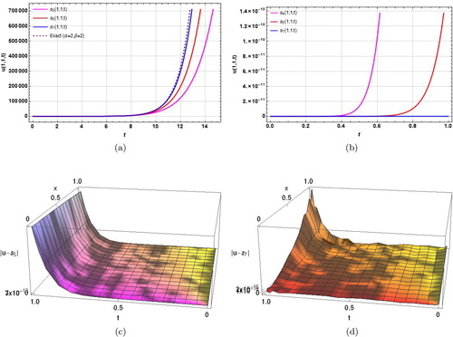
Table 1. Comparison of absolute errors for α = β = 2 at different time levels $t\le 1$.

x	t	NIPDTM		FRDTM
		$\left|u-s_5\right|$	$\left|u-s_7\right|$	$\left|u-s_5\right|$	$\left|u-s_7\right|$
0.25	0.50	1.22818E-15	0.00000E + 0	9.72184E-08	3.37159E-10
	0.75	2.39093E-13	6.93889E-18	1.66830E-06	1.29984E-08
	1.00	1.00849E-11	1.66533E-16	1.25746E-05	1.73809E-07
0.5	0.50	4.91274E-15	0.00000E + 0	3.88873E-07	1.34864E-09
	0.75	9.56374E-13	2.77556E-17	6.67322E-06	5.19938E-08
	1.00	4.03395E-11	6.66134E-16	5.02984E-05	6.95236E-07
0.75	0.50	1.10467E-14	5.55112E-17	8.74965E-07	3.03443E-09
	0.75	2.15183E-12	0.00000E + 0	1.50147E-05	1.16986E-07
	1.00	9.07638E-11	1.55431E-15	1.13171E-04	1.56428E-06

Table 2. mth order approximate solutions $S_m (m=5,7)$ of example 3.1 for $\alpha =\beta =1.5$ at different time levels $t\le 1$.

x	t	NIPDTM		FRDTM
		s5	s7	s5	s7
0.25	0.50	2.83204566869E-01	2.83204566922E-01	2.83125658991E-01	2.83125658991E-01
	0.75	3.02454881576E-01	3.02454884643E-01	3.02043708394E-01	3.02043708394E-01
	1.00	3.24456127246E-01	3.24456182967E-01	3.23110329539E-01	3.23110329539E-01
0.5	0.50	6.36250626260E-01	6.36250627946E-01	6.35610329539E-01	6.35610329539E-01
	0.75	7.20117322296E-01	7.20117422184E-01	7.16738630046E-01	7.16738630046E-01
	1.00	8.21254918294E-01	8.21256748649E-01	8.10021087743E-01	8.10021087743E-01
0.75	0.50	1.06267354670E + 0	1.06267355959E + 0	1.06048863004E + 0	1.06048863004E + 0
	0.75	1.26409119664E + 0	1.26409196524E + 0	1.25244718994E + 0	1.25244718994E + 0
	1.00	1.51710227178E + 0	1.51711644653E + 0	1.47789866862E + 0	1.47789866862E + 0

The absolute errors in the 5th and 7th order NIPDT solutions of $(1+1)$D STFH-like equation (12)(12) $$\begin{array}{c}{\mathcal{D}}_t^{\alpha }u(x,t)=\frac{x^2}{2}\frac{{\partial }^{\beta }u(x,t)}{\partial x^{\beta }}, u(x,0)=x, \frac{\partial u(x,0)}{\partial t}=x^2, 1<\alpha ,\beta \le 2\hfill \end{array}$$(12) for $\alpha =\beta =2,x,t\in (0,1)$ is depicted graphically in Figure 1(a) and Figure 1(b), respectively. The two-dimensional plots of different order solutions are depicted in Figure 1(c) for x = 1. It is evident from the above figures and Table 1 that the accuracy in the computed results increases rapidly with increasing order of approximation. The solution behavior of $(1+1)$D STFH-like equation (12)(12) $$\begin{array}{c}{\mathcal{D}}_t^{\alpha }u(x,t)=\frac{x^2}{2}\frac{{\partial }^{\beta }u(x,t)}{\partial x^{\beta }}, u(x,0)=x, \frac{\partial u(x,0)}{\partial t}=x^2, 1<\alpha ,\beta \le 2\hfill \end{array}$$(12) for $\alpha =\beta =2$ is depicted in Figure 1(e) and that for $\alpha =1.75,\beta =1.85$ is depicted in Figure 1(f). The two-dimensional plots of sixth order solutions for different values of α, β are depicted graphically in Figure 1(d) for $x=1,t\in (0,1)$.

Figure 1. The solution behavior of Example 3.1 obtained by using NIPDTM. (a) Absolute error in 5th order solution for α = β = 2. (b) Absolute error in 7th order solution α = β = 2. (c) Different order solutions for α = β = 2 for large time interval. (d) Sixth order solution for different values of α, β. (e) Eighth order solution for α = β = 2 with x = 1, t ∈ (0, 1). (f) Eighth order solution for α = 1.75, β = 1.85 with x = 1, t ∈ (0, 1).

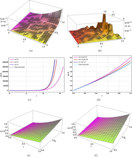
In Example 3.2, the absolute errors in mth order (m = 5, 7) solutions for $\alpha =\beta =2$ computed by both FRDTM and NIDTPM are reported in Table 3. The same order computed solutions by these methods for $\alpha =\beta =1.5$ are reported in Table 4. The conclusion from these two tables is analogous to Example 3.1. The two-dimensional plots, for $\alpha =\beta =2$ with $x=y=1$, of NIPDTM solutions of a different order (m = 3, 5, 7) are depicted graphically in Figure 2(a) for $t\le 16$ while the absolute errors in the mth order (m = 4, 5, 7) solutions are depicted graphically in Figure 2(b) for $t\le 1$. The absolute errors in the 5th/7th order NIPDTM solutions of $(2+1)$D STFH-like equation (23)(23) $$\{\begin{array}{c}U(x,y,0)=x^4+t{y}^4\hfill \\ U(x,y,\ell +1)={\mathcal{K}}^{-1}\left\{{\mu }^{2\alpha }\mathcal{K}\left\{\frac{x^2}{12}\frac{{\partial }^{\beta }U(x,y,\ell )}{\partial x^{\beta }}+\frac{y^2}{12}\frac{{\partial }^{\beta }U(x,y,\ell )}{\partial y^{\beta }}\right\}\right\},\ell >0\hfill \end{array}$$(23) for $\alpha =\beta =2,x,t\in (0,1),y=1$ are depicted graphically in Figure 2(c,d). The findings from the above figures and Table 3 show that the accuracy in the computed results increases rapidly with increasing order of approximation. The surface solution behaviors of Example 3.2 for $\alpha =1.25,\beta =1.5,\alpha =1.5,\beta =1.75$ and $\alpha =\beta =2$ are depicted graphically in ^{Figure 2} Figure 2(e,f,g). The two-dimensional plots of seventh order solutions for different values of α, β for $x=y=1,t\in (0,1)$ are depicted graphically in Figure 2(h).

Figure 2. The solution behavior of Example 3.2 obtained by using NIPDTM. (a) Comparison of different order solutions with exact solutions for α = β = 2, x = y = 1, t ≤ 16. (b) Absolute errors in different order solutions for α = β = 2, x = y = 1, t ≤ 1. (c) Absolute errors in 5th order solutions for α = β = 2, y = 1, t ≤ 1. (d) Absolute errors in 7th order solutions for α = β = 2, y = 1, t ≤ 1. (e) Seventh order solution behavior for α = 1.25, β = 1.5 at t = 1. (f) Seventh order solution behavior for α = 1.5, β = 1.75 at t = 1. (g) Seventh order solution behavior for α = 2, β = 2 at t = 1. (h) Plots of seventh order solutions for different α, β, x = y = 1.

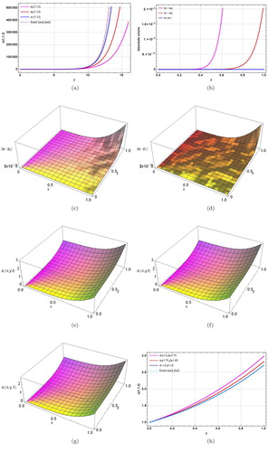
Table 3. Comparison of absolute errors in of example 3.2 for $\alpha =\beta =2$ at different time levels $t\le 1$.

x	y	t	NIPDTM		FRDTM
			$\left|u-s_5\right|$	$\left|u-s_7\right|$	$\left|u-s_5\right|$	$\left|u-s_7\right|$
0.25	0.25	0.50	2.07126E-15	0.00000E + 00	2.84922E-04	2.84831E-04
		0.75	2.74064E-13	3.46945E-18	6.87725E-04	6.86656E-04
		1.00	8.83028E-12	1.97758E-16	1.30839E-03	1.30219E-03
	0.50	0.50	3.21960E-15	0.00000E + 00	8.95365E-04	8.95183E-04
		0.75	4.98206E-13	6.93889E-18	2.74923E-03	2.74660E-03
		1.00	1.82848E-11	3.60822E-16	6.20299E-03	6.18517E-03
	0.75	0.50	8.21565E-15	2.77556E-17	3.54062E-03	3.54004E-03
		0.75	1.46955E-12	5.55112E-17	1.16824E-02	1.16730E-02
		1.00	5.92546E-11	1.05471E-15	2.74129E-02	2.73447E-02
0.50	0.25	0.50	3.19744E-14	0.00000E + 00	3.94831E-03	3.94695E-03
		0.75	4.16087E-12	2.77556E-17	8.94210E-03	8.92665E-03
		1.00	1.31830E-10	3.01148E-15	1.60397E-02	1.59521E-02
	0.50	0.50	3.31402E-14	0.00000E + 00	4.57503E-03	4.55730E-03
		0.75	4.38502E-12	5.55112E-17	1.10036E-02	1.09865E-02
		1.00	1.41285E-10	3.16414E-15	2.09343E-02	2.08351E-02
	0.75	0.50	3.80806E-14	0.00000E + 00	7.20400E-03	7.20216E-03
		0.75	5.35633E-12	5.55112E-17	1.99368E-02	1.99129E-02
		1.00	1.82254E-10	3.88578E-15	4.21442E-02	4.19946E-02

Table 4. mth order approximate solutions $S_m (m=5,7)$ of example 3.2 for $\alpha =\beta =1.5$ at different time levels $t\le 1$.

x	y	t	NIPDTM		FRDTM
			s5	s7	s5	s7
$\frac{1}{4}$	$\frac{1}{4}$	$\frac{1}{2}$	6.2446916961E-03	6.2446916963E-03	6.2345067984E-03	6.2434077587E-03
		$\frac{3}{4}$	7.6193202321E-03	7.6193202398E-03	7.5825287126E-03	7.6125694535E-03
		1	9.1436779259E-03	9.1436780318E-03	9.0503717796E-03	9.1215794619E-03
	$\frac{1}{2}$	$\frac{1}{2}$	3.6928879479E-02	3.6928879480E-02	3.6883570437E-02	3.6892471398E-02
		$\frac{1}{2}$	5.5471396904E-02	5.5471396980E-02	5.5254034939E-02	5.5284075680E-02
		1	7.5967840601E-02	7.5967841936E-02	7.5293255827E-02	7.5364463510E-02
	$\frac{3}{4}$	$\frac{1}{2}$	1.7147903698E-01	1.7147903700E-01	1.7119357385E-01	1.7120247481E-01
		$\frac{3}{4}$	2.6741365335E-01	2.6741365454E-01	2.6595689541E-01	2.6598693616E-01
		1	3.7549934716E-01	3.7549936855E-01	3.7081629472E-01	3.7088750240E-01
$\frac{1}{2}$	$\frac{1}{4}$	$\frac{1}{2}$	7.1882304358E-02	7.1882304382E-02	7.1589199993E-02	7.1874030722E-02
		$\frac{3}{4}$	7.9608995644E-02	7.9608996569E-02	7.8596924467E-02	7.9558228178E-02
		1	8.9231345700E-02	8.9231358146E-02	8.6766956899E-02	8.9045602733E-02
	$\frac{1}{2}$	$\frac{1}{2}$	1.0256649214E-01	1.0256649217E-01	1.0223826363E-01	1.0252309436E-01
		$\frac{3}{4}$	1.2746107232E-01	1.2746107331E-01	1.2626843069E-01	1.2722973440E-01
		1	1.5605550838E-01	1.5605552205E-01	1.5300984095E-01	1.5528848678E-01
	$\frac{3}{4}$	$\frac{1}{2}$	2.3711664964E-01	2.3711664969E-01	2.3654826704E-01	2.2891052675E-01
		$\frac{3}{4}$	3.3940332876E-01	3.3940333087E-01	3.3697129117E-01	3.3793259488E-01
		1	4.5558701493E-01	4.5558704866E-01	4.4853287984E-01	4.5081152567E-01

In Example 3.3, it is evident from Table 5 and Figure 3 that the computed results for $(3+1)$D STFH-like equation using NIPDTM are more accurate in comparison to FRDT solutions for the same order of approximation. Table 6 reports fifth/seventh order solutions computed by using both of these methods.

Table 5. Comparison of absolute errors in of example 3.3 for $\alpha =\beta =2$ at different time levels $t\le 1$.

x	y	t	NIPDTM		FRDTM
			$\left|u-s_5\right|$	$\left|u-s_7\right|$	$\left|u-s_5\right|$	$\left|u-s_7\right|$
0.25	0.25	0.50	1.76240E-15	1.38778E-17	3.72898E-06	1.64884E-08
		0.75	3.58977E-13	1.38778E-17	4.34679E-05	4.29938E-07
		1.00	1.56160E-11	2.49800E-16	2.50406E-04	4.37446E-06
	0.50	0.50	5.55112E-15	2.77556E-17	8.10786E-06	3.57157E-08
		0.75	1.11472E-12	5.55112E-17	9.52899E-05	9.37410E-07
		1.00	4.80304E-11	7.77156E-16	5.53249E-04	9.59825E-06
	0.75	0.50	1.19349E-14	0.00000E + 00	1.54060E-05	6.77611E-08
		0.75	2.37421E-12	1.11022E-16	1.81660E-04	1.78320E-06
		1.00	1.02054E-10	1.55431E-15	1.05799E-03	1.83046E-05
0.50	0.25	0.50	5.55112E-15	2.77556E-17	8.10786E-06	3.57157E-08
		0.75	1.11472E-12	5.55112E-17	9.52899E-05	9.37410E-07
		1.00	4.80304E-11	7.77156E-16	5.53249E-04	9.59825E-06
	0.50	0.50	9.38138E-15	0.00000E + 00	1.24867E-05	5.49429E-08
		0.75	1.87039E-12	1.11022E-16	1.47112E-04	1.44488E-06
		1.00	8.04447E-11	1.33227E-15	0.000856092	1.48220E-05
	0.75	0.50	1.56541E-14	1.11022E-16	1.97849E-05	8.69884E-08
		0.75	3.12994E-12	1.11022E-16	2.33482E-04	2.29067E-06
		1.00	1.34469E-10	2.22045E-16	1.36083E-03	2.35283E-05

Table 6. mth order approximate solutions $S_m (m=5,7)$ of example 3.3 for z = 0.2, $\alpha =\beta =1.5$ at different time levels $t\le 1$.

x	y	t	NIPDTM		FRDTM
			s5	s7	s5	s7
$\frac{1}{4}$	$\frac{1}{4}$	$\frac{1}{2}$	9.11325516424E-02	9.11325517558E-02	8.90612789699E-02	9.09510447640E-02
		$\frac{3}{4}$	1.59145637609E-01	1.59145644622E-01	1.51748089921E-01	1.58126049476E-01
		1	2.42924291632E-01	2.42924424296E-01	2.24268660422E-01	2.39386786775E-01
	$\frac{1}{2}$	$\frac{1}{2}$	2.47648268008E-01	2.47648270106E-01	2.41413734567E-01	2.46724527262E-01
		$\frac{1}{2}$	4.31131211919E-01	4.31131341226E-01	4.08055982555E-01	4.25979907899E-01
		1	6.62586763244E-01	6.62589208685E-01	6.02226814513E-01	6.44713156071E-01
	$\frac{3}{4}$	$\frac{1}{2}$	5.14976838140E-01	5.14976853858E-01	4.99405010157E-01	5.12011775471E-01
		$\frac{3}{4}$	9.05648854090E-01	9.05649827897E-01	8.46452827418E-01	8.89000660351E-01
		1	1.41439389097E + 0	1.41441241948E + 0	1.25518338854E + 0	1.35603751104E + 0
$\frac{1}{2}$	$\frac{1}{4}$	$\frac{1}{2}$	2.47648268008E-01	2.47648270106E-01	2.41413734567E-01	2.46724527262E-01
		$\frac{3}{4}$	4.31131211919E-01	4.31131341226E-01	4.08055982555E-01	4.25979907899E-01
		1	6.62586763244E-01	6.62589208685E-01	6.02226814513E-01	6.44713156071E-01
	$\frac{1}{2}$	$\frac{1}{2}$	4.04163984373E-01	4.04163988456E-01	3.93766190165E-01	4.02498009760E-01
		$\frac{3}{4}$	7.03116786229E-01	7.03117037831E-01	6.64363875188E-01	6.93833766322E-01
		1	1.08224923485E + 0	1.08225399307E + 0	9.80184968604E-01	1.05003952536E + 0
	$\frac{3}{4}$	$\frac{1}{2}$	6.71492554505E-01	6.71492572208E-01	6.51757465755E-01	6.67785257969E-01
		$\frac{3}{4}$	1.17763442840E + 0	1.17763552450E + 0	1.10276072005E + 0	1.15685451877E + 0
		1	1.83405636258E + 0	1.83407720387E + 0	1.63314154263E + 0	1.76136388034E + 0

4. Concluding remark

In this paper, a comparative study of analytical solutions of $(n+1)$-dimensional space-time fractional hyperbolic-like equations (with Caputo type fractional derivatives) has been made using two reliable semi-analytical methods: “new integral projected differential transform method (NIPDTM)” “and fractional reduced differential transform method (FRDTM)” Three test problems are used in order to illustrate the efficiency of these methods.

It is noted from Section 3 that the computed approximate series solutions for each problem with β = 2 are in excellent agreement with thoset obtained by modified HAM (Yin et al., 2015), DTM (Secer, 2012), ADM (Momani, 2005), HDM (Atangana & Alabaraoye, 2013), LHAM (Gupta and Kumar, 2012), FRDTM (Singh & Srivastava, 2015), VIM (Molliq et al., 2009; Yin et al., 2013), variable separation method (Zhang et al., 2016), and approaches to the exact solutions. The computed solutions from either method are obtained in terms of an infinite power series that converges to the exact solutions. The application of FRDTM is very easy, efficient, valuable and suitable for getting approximate solutions of (non)linear fractional PDEs. The NIPDTM is more general and it provides better accuracy in the results in compression to FRDTM, for the same order of approximations, i.e. NIPDT solutions converge to the exact solutions faster than the FRDT solutions.

Disclosure statement

No potential conflict of interest was reported by the authors.

References

- Agrawal, O. P. (2002). Solution for a fractional diffusionwave equation defined in a bounded domain. Nonlin. Dyn, 29, 145–155.
- Andrezei, H. (2002). Multi-dimensional solutions of space-time-fractional diffusion equations. Proc. R. Soc. Lond., Ser. A, Math. Phys. Eng. Sci, 458(2002), 429–450.
- Arshad, M., Lu, D., & Wang, J. (2017). (N + 1)-dimensional fractional reduced differential transform method for fractional order partial differential equations. Communications in Nonlinear Science and Numerical Simulation, 48, 509–519.
- Atangana, A., & Alabaraoye, E. (2013). Exact Solutions Fractional Heat-Like and Wave-Like Equations with Variable Coefficients. Scientific Reports, 2(2), 663–667. doi:10.4172/scientificreports.633
- Atangana, A., & Baleanu, D. (2016). New fractional derivatives with nonlocal and non-singular kernel: Theory and application to heat transfer model. Thermal Science, 20(2), 763–769.
- Baleanu, D., Machado, J. A. T., & Luo, A. C. (2012). Fractional dynamics and control. Springer.
- Carpinteri, A., & Mainardi, F. (1997). Fractals and fractional calculus in continuum mechanics. Springer Verlag, Wien, New York.
- El-Sayed, A. M. A. (1996). Fractional - order diffusionwave equation. International Journal of Theoretical Physics, 35(2), 311–322.
- Fu, Z.-J., Chen, W., & Yang, H.-T. (2013). Boundary particle method for Laplace transformed time fractional diffusion equations. Journal of Computational Physics, 235, 52–66.
- Fu, Z.-J., Chen, W., & Ling, L. (2015). Method of approximate particular solutions for constant- and variable-order fractional diffusion models. Engineering Analysis with Boundary Elements, 57, 37–46.
- Gupta, V. G., & Kumar, P. (2012). Applications of laplace homotopy analysis method for solving fractional heat- and wave-like equations. Global Journal of Science Frontier Research Mathematics and Decision Sciences, 12(6), 39–48.
- Hanyga, A. (2002). Multidimensional solutions of time - fractional diffusion wave equations. Proc. R. Soc. Lond. A, 458, 933–957.
- He, J. H. (1998). Nonlinear oscillation with fractional derivative and its applications. Int. Conf. Vibrating Engg’98, Dalian, 288–291.
- He, J. H. (1999). Homotopy perturbation technique. Comput. Methods Appl. Mechanics Engg, 178(3-4), 257–262.
- Herzallah, M. A. E., A.M.A, E.-S., & Baleanu, D. (2010). On the fractional- order diffusion - wave process, Rom. Journ. Phys. 55, 274–284.
- Holliday, J. R., Rundle, J. B., Tiampo, K. F., Klein, W., & Donnellan, A. (2006). Modification of the pattern informatics method for forecasting large earthquake events using complex eigen factors. Tectonophysics, 413(1-2), 87–91.
- Jafari, H., & Momani, S. (2007). Solving fractional diffusion and wave equations by modified homotopy perturbation method. Physics Letters A, 370(5-6), 388–396.
- Jesus, I. S., & Machado, J. A. T. (2008). Fractional control of heat diffusion systems. Nonlinear Dynamics, 54(3), 263–282.
- Kashuri, A., & Fundo, A. (2013). A new integral transform. Adv Theoretical Appl Math, 8(1), 27–43.
- Kashuri, A., Fundo, A., & Kreku, M. (2013). Mixture of a new integral transform and homotopy perturbation method for solving nonlinear partial differential equations. Advances in Pure Mathematics, 03(03), 3, 317–23.
- Khader, M., Kumar, S., & Abbasbandy, S. (2016). Fractional homotopy analysis transforms method for solving a fractional heat - like physical model. Walailak J Sci & Tech, 13(5), 337–353.
- Klafter, J., Blumen, A., & Zumofen, G. (1984). Fractal behavior in trapping and reaction: a random walk study. Journal of Statistical Physics, 36(5-6), 561–578.
- Kunjan, S., Twinkle, S., & Kilicman, A. (2016). Combination of integral and projected differential transform methods for time-fractional gas dynamics equations. Ain Shams Eng J, 2017 doi:10.1016/j.asej.2016.09.012
- Magin, R. L. (2006). Fractional Calculus in Bioengineering, Begell House Publisher, Inc. Connecticut.
- Mainardi, F. (1971). Fractional calculus: Some basic problems in continuum and statistical mechanics, in: A. carpinteri, F. Mainardi (Eds.), Fractals and Fractional Calculus in Continuum Mechanics, SpringerVerlag, New York, 291–348.
- Mainardi, F. (1996). Fractional relaxation oscillation and fractional diffusion wave phenomena. Chaos, Solitons and Fractals, 7(9), 1461–1477.
- Manolis, G. D., & Rangelov, T. V. (2006). Non-homogeneous elastic waves in solid: notes on the vector decomposition technique. Soil Dyn Earthq Eng, 26(10), 952–959.
- Mentrelli, A., & Pagnini, G. (2015). Front propagation in anomalous diffusive media governed by time - fractional diffusion. Journal of Computational Physics., 293, 427–441.
- Miller, K. S., & Ross, B. (1993). An Introduction to the fractional calculus and fractional differential equations. Wiley, New York, 1993.
- Molliq, Y. R., Noorani, M. S. M., & Hashim, I. (2009). Variational iteration method for fractional heat- and wave-like equations. Nonlinear Analysis: Real World Applications, 10(3), 1854–1869.
- Momani, S. M. (2005). Analytical approximate solution for fractional heat-like and wave-like equations with variable coefficients using the decomposition method. Applied Mathematics and Computation, 165(2), 459–472.
- Özis, T., & Agirseven, D. (2008). He’s homotopy perturbation method for solving heat-like and wave-like equations with variable coefficients. Phys Lett A, 372, 5944–5950.
- Pandey, R. K., & Mishra, H. K. (2017). Semi- analytic numerical method for solution of time-space fractional heat and wave type equations with variable coefficients. Open Physics, 15(1), 74–86.
- Pang, G., Chen, W., & Fu, Z. (2015). Space-fractional advection-dispersion equations by the Kansa method. Journal of Computational Physics, 293, 280–296.
- Secer, A. (2012). Approximate analytic solution of fractional heat-like and wave-like equations with variable coefficients using the differential transforms method. Advances in Difference Equations, 2012(1), 198. doi:10.1186/1687-1847-2012-198.
- Singh, B. K., & Srivastava, V. K. (2015). Approximate series solution of multi-dimensional, time fractional-order (heat-like) diffusion equations using FRDTM. R. Soc. Open Sci. 29, 2(4), 140511. doi:10.1098/rsos.140511.
- Singh, B. K., & Kumar, P. (2018). Homotopy perturbation transform method for solving fractional partial differential equations with proportional delay. Sema Journal, 75(1), 111–125.
- Singh, B. K., & Kumar, P. (2017). Extended Fractional Reduced Differential Transform for Solving Fractional Partial Differential Equations with Proportional Delay. International Journal of Applied and Computational Mathematics, 3(S1), 631–649.
- Singh, B. K., & Kumar, P. (2017). Fractional variation iteration method for solving fractional partial differential equations with proportional delay. Int. J. Differ. Equ., 2017, 5206380. doi:10.1155/2017/5206380.
- Singh, B. K., & Kumar, P. (2016). FRDTM for numerical simulation of multi-dimensional, time-fractional model of Navier-Stokes equation. Ain Shams Engineering Journal, doi:10.1016/j.asej.2016.04.009.
- Singh, J., Kumar, D., & Kilicman, A. (2013). Application of homotopy perturbation Sumudu transform method for solving heat and wave-like equations. Malaysian J Math. Sc, 7(1), 79–95.
- Shou, D. H., & He, J. H. (2008). Beyond adomian method: the variational iteration method for solving heat-like and wave-like equations with variable coefficients. Phys Lett A, 372(3), 233–237.
- Taghizadeh, N., & Noori, S. R. M. (2017). Reduced differential transform method for solving parabolic-like and hyperbolic-like equations. SeMA Journal, 74(4), 559. doi:10.1007/s40324-016-0101-1.
- Tarasov, V. E. (2008). Fractional vector calculus and fractional Maxwell’s equations. Anna. of Phys, 323(11), 2756–2778.
- Tang, B., Wang, X., Wei, L., & Zhang, X. (2014). Exact solutions of fractional heat-like and wave-like equations with variable coefficients. International Journal of Numerical Methods for Heat & Fluid Flow, 24(2), 455–467. doi:10.1108/HFF-05-2012-0106.
- Wazwaz, A. M., & Goruis, A. (2004). Exact solution for heat-like and wave-like equations with variable coefficient. Journal of Applied Mathematics and Computing., 149, 51–59.
- Xu, H., & Cang, J. (2008). Analysis of a time fractional wave-like equation with the homotopy analysis method. Phys. Lett. A, 372(8), 1250–1255.
- Yin, F., Song, J., & Cao, X. (2013). A general iteration formula of VIM for fractional heat- and wave-like equations. Journal of Applied Mathematics, 2013, 428079. doi:10.1155/2013/428079.
- Yin, X. B., Kumar, S., & Kumar, D. (2015). A modified homotopy analysis method for solution of fractional wave equations. Advances in Mechanical Engineering, 7(12), 1–8.
- Zhang, X., Zhao, J., Liu, J., & Tang, B. (2014). Homotopy perturbation method for two dimensional time-fractional wave equation. Applied Mathematical Modelling, 38(23), 5545–5552.
- Zhang, S., Zhu, R., & Zhang, L. (2016). Exact solutions of time fractional heat-like and wave-like equations with variable coefficients. THERMAL Science, 20(suppl. 3), 689–S693.