Mathematical modelling for a fabrication–inventory problem with scrap, an acceptable stock-out level, stochastic failures and a multi-shipment policy

Abstract

While planning for batch manufacturing, determining the optimal runtime that minimizes total system costs is equally important and so is maintaining high product quality, keeping the batch process environment free of disruption, and ensuring timely delivery of end products to meet market demand. Owing to the imperfect nature of the fabrication process, both the production of random scrap and machine failures are inevitable and require special treatment. Permitting an acceptable level of shortages with backordering is often considered an effective approach to reduce inventory costs and lower the total system costs. Moreover, for delivering end products, a periodic multi-shipment policy is commonly adopted in real supply chain systems. To cope with the aforementioned realistic factors, this study explores a fabrication–inventory problem that considers scrap items, an acceptable level of stock outs with backordering, stochastic machine failures, and a multi-shipment policy.

A mathematical model is built to accurately represent the problem. An optimization method along with an algorithm is presented to derive optimal production uptime that minimizes total system costs. Using a numerical example, we demonstrate that this precise model and its solution process can not only provide an optimal decision, but also reveal diverse and valuable system characteristics including (1) details of cost components of the system and (2) the individual and joint impact of system factors, such as product quality, service-level constraints, machine failures, number of deliveries, and uptime in the proposed problem. Without such an in-depth exploration, these important system characteristics remain inaccessible and unknown to production managers.

Keywords:

• Optimization
• Mathematical modelling
• Fabrication–inventory problem
• Machine failure
• Backlogging
• Scrap
• Multi-shipment policy

1. Introduction

A fabrication–inventory problem considering scrap items, an acceptable level of stock outs with backordering, stochastic machine failures, and a multi-shipment policy is investigated. In batch production planning, Taft (1918) first presented the most economic fabrication batch that minimizes the long-run system costs, wherein a mathematical model was used under simple assumptions such as a perfect fabrication process and a continuous end-item issuing plan. However, in most manufacturing systems, owing to the imperfect nature of the fabrication process, production of random scrap and stochastic machine failures are both inevitable and require special treatment. Lee and Rosenblatt (1987) explored a production system with the objective of simultaneously deciding production cycle length and inspection plan. The authors also presented a relationship that helped decide the maintenance’s effectiveness by the inspection plan. Groenevelt et al. (1992) studied the impacts of machine failures and its consequent corrective actions to the optimal batch size decision. Two distinct stock control policies dealing with breakdown occurrence were studied. The first is the no-resumption (NR) rule, and it assumes that the disrupted batch will not be resumed even after the machine is restored. The second is the abort–resume (AR) discipline, which assumes that after the machine is restored and if the level of current stocks falls below a preset threshold point, then production of the disrupted batch is resumed right away. As a result, they provided a closed-form approximate for batch size equations and for system costs. Kim and Hong (1997) investigated a manufacturing system with a failure-prone machine with general lifetime distribution. Therein, the time between machine failures is generally distributed and the failure machine is under repair immediately. They analysed and discussed how to derive optimal batch size and prove its uniqueness, according to various assumed failure-rate functions. Abboud (2001) explored a production–inventory system with facility breakdown, wherein both breakdown rate and repairing time were assumed random variables, and both time-to-failure and repairing time are discrete and follow geometric distribution. Accordingly, a Markov chain approach along with a proposed algorithm was utilized to portray and resolve the problem. Chakraborty et al. (2008) studied a generalized unreliable economic manufacturing quantity (EMQ)-based system, in which the machine may shift to out-of-control state from in-control state at any time. During uptime, when a breakdown happens, the machine is immediately under a corrective repair. Based on the assumption that time-to-failure, corrective and preventive repair times all follow an arbitrary probability distribution, they developed and formulated the model for the problem. Through a numerical example, they showed how to derive the optimal runtime and analyse the joint effects of process deterioration, facility failures and repairs on the optimal decisions. Khan et al. (2014) developed an integrated mathematical model to help decide the optimal inventory policy for a vendor–buyer supply chain system that minimizes the combined cost of the system. Their policy took into account the buyer’s errors in quality screening and the vendor’s learning in production. A numerical example was used to demonstrate the applicability of their model. Discussion and suggestion were also provided that touched on investment justification of product and process design, personnel training and directions for future study. Extra studies (Moinzadeh & Aggarwal, 1997; Jaber, 2006; Rivera-Gómez et al., 2013; Abilash & Sivapragash, 2016; Jawla & Singh, 2016; Rakyta et al., 2016; Zahedi et al., 2016; Abubakar et al., 2017; Chiu et al., 2017; Khalili et al., 2017; Liu et al., 2017; MohanDas et al., 2017) have also been carried out to address diverse unreliable and imperfect features of fabrication systems.

Furthermore, for delivering finished products, a periodic multi-shipment plan is commonly adopted in most real supply chain systems. Schwarz (1973) determined an optimal inventory policy that minimizes system costs for a single-warehouse multiple retailer supply-chain system. Heuristic approaches were developed in solution processes for the general problem. As a result, certain essential properties for the system were disclosed and the optimal policy was derived. Banerjee (1986) studied a vendor and purchaser integrated system with the aim of determining a joint economic batch size that minimizes the joint system costs. The author thought that with a proper adjustment in price, the obtained optimal ordering decision can be beneficial to both parties. Hall (1996) explored the effects of features of a delivery system on economic order quantity (EOQ) and economic production quantity (EPQ) decisions. Through development of inventory characteristic curves, the system attributes within the proposed integrated production–delivery systems and their effects on EOQ/EPQ formulas were analysed. Certain valuable conclusions were drawn that can help managerial decision-making. Buscher and Lindner (2005) used an optimization method to derive the most economic manufacturing and rework quantities for a fabrication system featuring rework and multiple equal-sized deliveries. A numerical example along with sensitivity analysis under diverse values of system variables was provided to verify their method and demonstrate the applicability of their results. Archetti et al. (2013) proposed a heuristic algorithm to explore an effective plan to distribute free newspapers from a vendor to mass transportation centres, such bus, train, or subway stations. The main objectives were to minimize (i) the vehicle trips needed to deliver all newspapers from the vendor, and (ii) the time needed for all newspapers to be received by readers. A formulation, heuristic algorithms and the hybrid approach were used to resolve their routing–inventory problem with an additional constraint on vendor’s fabrication schedule. Real-world data were also used and compiled to test and demonstrate the performance of their approaches. Additional works that focused on diverse aspects of integrated fabrication–delivery systems have also been conducted elsewhere (Balaji et al., 2016; Caiazza et al., 2016; Chiu et al., 2016; Florea Ionescu et al., 2016; Jindal & Solanki, 2016; Mičieta et al., 2016; Raj & Prabha, 2016; Razmi et al., 2016; Afshar-Nadjafi & Afshar-Nadjafi, 2017; Gopinath et al., 2017; Settanni et al., 2017).

Furthermore, permitting an acceptable level of shortages with backordering is often considered an effective approach to reducing inventory costs and lowering total system costs, given that the minimum service level is retained. Meaning not to allow abusive shortage causes lower customer satisfaction and turns into loss of future sales (due to loss of goodwill). Bashyam and Fu (1998) determined the optimal (s, S) ordering policy for inventory systems featuring variable lead times and under the service-level constraint. They considered that orders are permitted to cross in time. Accordingly, a simulation approach using numerous data sets was proposed to search for feasible suboptimal solution to the problem. Chiu (2006) investigated the effect of service-level constraint on an EPQ-based system with random scrap. The author first proved that the expected system cost for the proposed system with permissible backlogging is less than or equal to that in the same system without backlogging. Then, the relationship between so-called “imputed backorder cost” and maximal backlogging level was derived to help decide whether a preset service level can be achieved. Lastly, an equation was proposed to compute unit intangible cost for backordering, and it can also be used to find a new optimal order policy that minimizes system costs and satisfies the preferred service level. Numerical demonstration was provided to show applicability of his research result. Cardós et al. (2013) aimed at improving inventory management of repairable components for an airline company. They proposed a heuristic to resolve the existing problem with the purpose of reducing the fill rate and stock level of the repairable components. As a result, they showed that the proposed heuristic outperforms the current method and leads to a considerable reduction in inventory. Extra research (de Kok, 1985; Tempelmeier, 2007; Selçuk & Ağralı, 2013; Jaggi et al., 2016; Salemi, 2016; Oblak et al., 2017) has also been carried out to address diverse aspects of backordering and service-level constraint of fabrication systems.

As little attention has been paid to the exploration of combined effects of scrap, an acceptable stock-out level, stochastic failures and a multi-shipment policy on the optimal uptime decision for a fabrication–inventory system, the present research aims to fill the research gap.

2. The proposed fabrication–inventory problem

This section provides the description, assumption and mathematical modelling and analysis for the proposed fabrication–inventory problem featuring backordering of the acceptable shortages (i.e. under service-level constraint), Poisson machine failures, a multi-shipment policy and scrap. The system has an annual fabrication rate P to satisfy the buyer’s annual demand rate λ, and its fabrication process may generate x percentage of scrap randomly. In order to maintain an acceptable service rate (1 – α)%, certain shortages are permitted and backordered, where the maximum permitted percentage α denotes the minimum permissible stock-out time in a cycle. Also, due to the discontinuous nature of the product delivery policy, the permitted backlogging B is supplied by a single shipment made in the end of t₄′. Moreover, this specific system is subject to a Poisson facility failure with mean = β per year. If a machine breakdown happens, an abort–resume policy is implemented and the failure facility is right away under repair. Repair time t_r is assumed to be constant. Once the repair task is accomplished, the fabrication of disturbed batch is resumed immediately. When the production uptime finishes, a multi-shipment plan is adopted to distribute end items. The basic assumption of (P – d – λ) > 0 has to hold to guarantee the status of positive stocks in any replenishment cycle. Definition of other parameters is provided as follows:

Q = batch size,

t₄′ = uptime in which shortages are backordered,

t₁′ = uptime in which positive stocks are piled up,

T₁ = (t₄′ + t₁′), production uptime – the decision variable,

t₂′ = time to distribute on-hand finished items,

t₃′ = time to accumulate permissible backlogging,

T′ = fabrication cycle length in the case that a failure happens in uptime,

t_n′ = interval of time between two consecutive deliveries,

t = time to a failure occurs,

B = maximal level of permissible backlogging,

b = unit backorder cost,

M = fixed machine repair cost,

d = Px, production rate of scrap,

H₀ = the level of backlogging when a failure happening in t₄′,

H = the level of finished stock in the end of T₁,

H₁ = the level of finished stock when a failure happening within [t₄′, T₁],

h = unit stock holding cost,

h₃ = unit safety stock holding cost,

C = fabrication cost per product,

K = setup cost,

C_S = unit disposal cost per scrap,

K₁ = fixed cost per delivery,

C₁ = unit cost per safety stock,

C_T = unit distribution cost,

g = t_r, fixed machine repair time,

I(t) = on-hand inventory/backlog level at time t,

I_S(t) = on-hand scrap level at time t,

t₄ = uptime in which shortages are backordering in a system without breakdown,

t₁ = uptime in which positive stocks are piling up in a system without breakdown,

t₂ = time to distribute on-hand finished items in a system without breakdown,

t₃ = time to accumulate permissible backlogging in a system without breakdown,

t_n = interval of time between two consecutive shipments in a system without breakdown,

T = cycle length in a system (whether or not a breakdown happening),

TC₁(T₁) = total cost per cycle in the case that a breakdown happens in t₄′,

TC₂(T₁) = total cost per cycle in the case that a breakdown happens within [t₄′, T₁]

TC₃(T₁) = total cost per cycle in the case that no breakdown happens,

E[TC₁(T₁)] = expected total cost per cycle in the case that a breakdown happens in t₄′,

E[TC₂(T₁)] = expected total cost per cycle in the case that a breakdown happens within [t₄′, T₁]

E[TC₃(T₁)] = expected total cost per cycle in the case that no breakdown happens,

TCU(T₁) = total system cost per unit time whether a breakdown happening or not,

E[TCU(T₁)] = expected total system cost per unit time whether a breakdown happening or not.

Due to the stochastic nature of machine failures, the following distinct conditions need to be explored.

2.1. Condition 1: a stochastic failure happens in t₄′

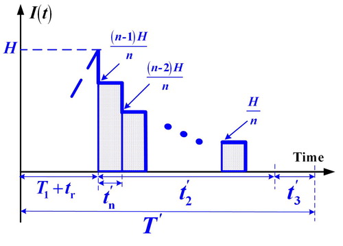
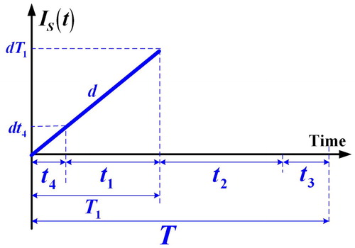
When a random facility breakdown happens, the backlog level stays at H₀ for a period of t_r until completion of the repair task (see Figure 1). Then, the disturbed batch is resumed at once. Because of the discontinuous nature of the end-item shipping policy, the permissible backlogging B is satisfied by a single shipment made in the end of t₄′. In the uptime period t₁′, on-hand finished stocks begin to grow up to level H. The on-hand level of scraps in the proposed system with a breakdown happening in t₄′ is illustrated in Figure 2. It can be seen that the maximum scraps is dT₁ (Figure 2). Next, n fixed quantity instalments of on-hand stocks are distributed at a fixed interval of time t_n′ during t₂′ (Figure 3). Any product demand after the end of t₂′ becomes shortage and is backordered in t₃′. When the backlog level reaches (B – λt₄′), then next replenishment cycle starts (Figure 1).

Figure 1. The on-hand inventory/backlog level at time t in the proposed system with a breakdown happening in t₄′.

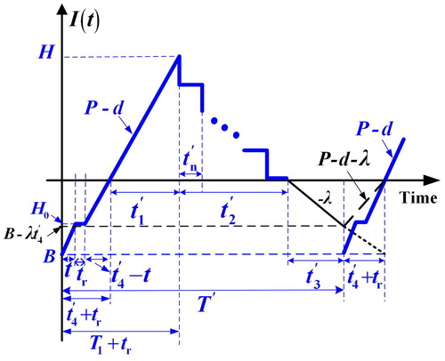
Figure 2. The on-hand scrap level at time t in the proposed system with a breakdown happening in t₄′.

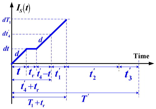
Figure 3. The on-hand finished product level in distribution time t₂′ in the proposed system with a breakdown happening in t₄′.

The following basic equations in this breakdown happening in t₄′ case can be observed from Figures 1 to 3: (1) $$t_4^{\prime }=\frac{B}{\left(P-d\right)}$$(1) (2) $$t_1^{\prime }=\frac{H}{\left(P-d\right)}$$(2) (3) $$T_1=\left(t_4^{\prime }+t_1^{\prime }\right)=\frac{Q}{P}$$(3) (4) $$H_0=B-\left(P-d\right)t$$(4) (5) $$H=\left(P-d\right)t_1^{\prime }$$(5) (6) $$t_3^{\prime }=\frac{B-\lambda t_4^{\prime }}{\lambda }$$(6) (7) $$T^{\prime }=\left(\sum _{i=1}^4{t}_i^{\prime }\right)+t_r$$(7) (8) $$t_2^{\prime }=T^{\prime }-\left(t_1^{\prime }+t_3^{\prime }+t_4^{\prime }+t_r\right)$$(8) (9) $$t_n^{\prime }=\frac{t_2^{\prime }}{n}$$(9)

In t₂′, the sum of inventories (Figure 3) are as follows (Chiu et al., 2016): (10) $$\left(\frac{1}{n^2}\right)\left(\sum _{i=1}^{n-1}i\right)H{t}_2^{\prime }=\left(\frac{n-1}{2n}\right)H{t}_2^{\prime }$$(10)

Total cost per cycle TC₁(T₁), in the case that a breakdown happens in t₄′, is composed of the variable fabrication cost, production setup cost, disposal cost for scraps, breakdown repair cost, variable cost and holding cost for safety stocks, holding cost for products fabricated in t₄′, backordering cost during t₃′, t₄′, and t_r, fixed and variable costs for items transported during t₂′ and in the end of t₄′, and holding cost for finished and scrap items during t₁′ and t₂′. (11) $$\begin{array}{c}T{C}_1\left(T_1\right)=C\left(T_1{P}_1\right)+K+C_{S}x\left(T_{1}P\right)+M\\ +\left[C_1\left(\lambda t_r\right)+h_3(\lambda t_r)\left(t+\frac{t_r}{2}\right)\right]\\ +b\frac{B}{2}\left(t_3^{\prime }+t_4^{\prime }+t_{\mathrm{r}}\right)+h\left[\frac{B}{2}{t}_4^{\prime }+\left[\left(P-d\right)t\right]t_r\right]\\ +K_1+n{K}_1+C_T\left[\left(1-x\right)\left(T_{1}P\right)+\lambda t_r\right]\\ +h\left[\frac{H}{2}\left(t_1^{\prime }\right)+\left(\frac{n-1}{2n}\right)H{t}_2^{\prime }+\left(dt\right)t_r+\frac{d{T}_1}{2}\left(T_1\right)\right]\end{array}$$(11)

Applying the expected value E[x] to take into account of the randomness of the scrap rate, also substituting Equations (1)–(10) in Equation (11)(11) $$\begin{array}{c}T{C}_1\left(T_1\right)=C\left(T_1{P}_1\right)+K+C_{S}x\left(T_{1}P\right)+M\\ +\left[C_1\left(\lambda t_r\right)+h_3(\lambda t_r)\left(t+\frac{t_r}{2}\right)\right]\\ +b\frac{B}{2}\left(t_3^{\prime }+t_4^{\prime }+t_{\mathrm{r}}\right)+h\left[\frac{B}{2}{t}_4^{\prime }+\left[\left(P-d\right)t\right]t_r\right]\\ +K_1+n{K}_1+C_T\left[\left(1-x\right)\left(T_{1}P\right)+\lambda t_r\right]\\ +h\left[\frac{H}{2}\left(t_1^{\prime }\right)+\left(\frac{n-1}{2n}\right)H{t}_2^{\prime }+\left(dt\right)t_r+\frac{d{T}_1}{2}\left(T_1\right)\right]\end{array}$$(11) , and with additional derivations, E[TC₁(T₁)] becomes as follows: (12) $$\begin{array}{c}E\left[T{C}_1\left(T_1\right)\right]=C{T}_{1}P+K+C_{S}E\left[x\right]\left(T_{1}P\right)+M\\ +\left[C_1\left(\lambda t_r\right)+h_3(\lambda t_r)\left(t+\frac{t_r}{2}\right)\right]\\ +b\frac{B}{2}\left(\frac{B}{\lambda }+g\right)\\ +h\left[\frac{B^2}{2P\left(1-E\left[x\right]\right)}+Ptg+A_1\right]+K_1+n{K}_1\\ +C_T\left[T_{1}P\left(1-E\left[x\right]\right)+\lambda g\right]\\ -\frac{h}{n}\left[T_{1}B-\frac{B^2}{2P\left(1-E\left[x\right]\right)}-\frac{T_1^{2}P}{2}+A_1\right]\end{array}$$(12) where $$A_1=-\frac{T_1\lambda g}{2}+\frac{B\lambda g}{2P\left(1-E\left[x\right]\right)}+\frac{{\left[T_{1}P\left(1-E\left[x\right]\right)-B\right]}^2}{2\lambda }+\frac{T_1^{2}PE\left[x\right]}{2}-\frac{\lambda g^2}{2}$$

2.2. Condition 2: a stochastic failure happens within [t₄′, T₁]

When a random facility breakdown happens, the on-hand stock level at H₁ (see Equation (13)(13) $$H_1=\left(P-d\right)\left(t-t_4^{\prime }\right)$$(13) ) for a period of t_r until completion of the repair task (see Figure 4), then, interrupted batch is resumed at once to bring the stock level to H in the uptime t₁′. (13) $$H_1=\left(P-d\right)\left(t-t_4^{\prime }\right)$$(13)

Figure 4. The on-hand inventory/backlog level at time t in the proposed system with a breakdown happening in the period of [t₄′, T₁].

The on-hand level of scraps in the proposed system with a breakdown happening in the period of [t₄′, T₁] is depicted in Figure 5. It can be seen that the maximum scraps is d₁T₁ (Figure 5). Then, n fixed quantity instalments of on-hand stocks are distributed at a fixed interval of time t_n′ during t₂′ (Figure 4). In t₃′, any product demand becomes shortage and is backordered to the level of (B – λt₄′), then the next replenishment cycle begins (Figure 4). Because of the discontinuous nature of the product delivery policy, the permitted backlogging B is satisfied by a single shipment made in the end of t₄′. From Figures 3, 4, and 5, we verify that the aforementioned Equations (1)–(3) and (5)–(10) are still applicable for analysing the present model (i.e. for condition 2).

Figure 5. The on-hand scrap level at time t in the proposed system with a breakdown happening in the period of [t₄′, T₁].

The total cost per cycle in the case that a breakdown happens in the period of [t₄′, T₁], TC₂(T₁) (i.e. Equation (14)(14) $$\begin{array}{c}T{C}_2\left(T_1\right)=C\left(T_{1}P\right)+K+C_{S}x\left(T_{1}P\right)+M\\ +\left[C_1\left(\lambda t_r\right)+h_3(\lambda t_r)\left(t+\frac{t_r}{2}\right)\right]\\ +b\frac{B}{2}\left(t_3^{\prime }+t_4^{\prime }\right)+h\left(\frac{B}{2}{t}_4^{\prime }\right)+K_1+n{K}_1\\ +C_T\left[\left(1-x\right)\left(T_{1}P\right)+\lambda t_r\right]\\ +h\left[\frac{H}{2}\left(t_1^{\prime }\right)+H_1{t}_{\mathrm{r}}+\left(\frac{n-1}{2n}\right)H{t}_2^{\prime }+\left(dt\right)t_r+\frac{d{T}_1}{2}\left(T_1\right)\right]\end{array}$$(14) ) is composed of the variable fabrication cost, production setup cost, disposal cost for scraps, breakdown repair cost, variable cost and holding cost for safety stocks, holding cost for products fabricated in t₄′, backordering cost during t₃′, t₄′, and t_r, fixed and variable costs for items transported during t₂′ and in the end of t₄′, and holding cost for finished and scrap items during t₁′ and t₂′. (14) $$\begin{array}{c}T{C}_2\left(T_1\right)=C\left(T_{1}P\right)+K+C_{S}x\left(T_{1}P\right)+M\\ +\left[C_1\left(\lambda t_r\right)+h_3(\lambda t_r)\left(t+\frac{t_r}{2}\right)\right]\\ +b\frac{B}{2}\left(t_3^{\prime }+t_4^{\prime }\right)+h\left(\frac{B}{2}{t}_4^{\prime }\right)+K_1+n{K}_1\\ +C_T\left[\left(1-x\right)\left(T_{1}P\right)+\lambda t_r\right]\\ +h\left[\frac{H}{2}\left(t_1^{\prime }\right)+H_1{t}_{\mathrm{r}}+\left(\frac{n-1}{2n}\right)H{t}_2^{\prime }+\left(dt\right)t_r+\frac{d{T}_1}{2}\left(T_1\right)\right]\end{array}$$(14)

Applying the expected value E[x] to take into account the randomness of the scrap rate, and also substituting Equations (1)–(3), (5)–(10) and (13)(13) $$H_1=\left(P-d\right)\left(t-t_4^{\prime }\right)$$(13) in Equation (14)(14) $$\begin{array}{c}T{C}_2\left(T_1\right)=C\left(T_{1}P\right)+K+C_{S}x\left(T_{1}P\right)+M\\ +\left[C_1\left(\lambda t_r\right)+h_3(\lambda t_r)\left(t+\frac{t_r}{2}\right)\right]\\ +b\frac{B}{2}\left(t_3^{\prime }+t_4^{\prime }\right)+h\left(\frac{B}{2}{t}_4^{\prime }\right)+K_1+n{K}_1\\ +C_T\left[\left(1-x\right)\left(T_{1}P\right)+\lambda t_r\right]\\ +h\left[\frac{H}{2}\left(t_1^{\prime }\right)+H_1{t}_{\mathrm{r}}+\left(\frac{n-1}{2n}\right)H{t}_2^{\prime }+\left(dt\right)t_r+\frac{d{T}_1}{2}\left(T_1\right)\right]\end{array}$$(14) , and with additional derivations, E[TC₂(T₁)] becomes as follows: (15) $$\begin{array}{c}E\left[T{C}_2\left(T_1\right)\right]=C{T}_{1}P+K+C_{S}E\left[x\right]\left(T_{1}P\right)+M\\ +\left[C_1\left(\lambda t_r\right)+h_3(\lambda t_r)\left(t+\frac{t_r}{2}\right)\right]+b\left(\frac{B^2}{2\lambda }\right)\\ +K_1+n{K}_1+C_T\left[T_{1}P\left(1-E\left[x\right]\right)+\lambda g\right]\\ +h\left[\frac{B^2}{2P\left(1-E\left[x\right]\right)}+Ptg+A_1\right]\\ -\frac{h}{n}\left[T_{1}B-\frac{B^2}{2P\left(1-E\left[x\right]\right)}-\frac{T_1^{2}P}{2}+A_1\right]\end{array}$$(15)

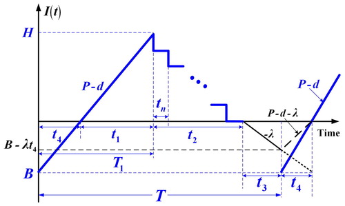
2.3. Condition 3: no failures happen during uptime T₁

When no facility breakdown happens during uptime, the on-hand stock level of finished products is displayed in Figure 6. The on-hand levels of scraps at time t and finished stocks during delivery time t₂ are illustration in Figures A-1 and A-2 in Appendix A. Similar basic formulas can also be found as shown in Appendix A.

Figure 6. The on-hand inventory/backlog level at time t in the proposed system with no breakdown happening in uptime.

Total cost per cycle in the case that no breakdown happens during uptime, TC₃(T₁) (i.e. Equation (16)(16) $$\begin{array}{c}T{C}_3\left(T_1\right)=C\left(T_{1}P\right)+K+C_{S}x\left(T_{1}P\right)+\left[C_1\left(\lambda t_r\right)+h_3(\lambda t_r)T\right]\\ +h\left(\frac{B}{2}{t}_4\right)+b\frac{B}{2}\left(t_3+t_4\right)\\ +K_1+n{K}_1+C_T\left(1-x\right)\left(T_{1}P\right)\\ +h\left[\frac{H}{2}\left(t_1\right)+\left(\frac{n-1}{2n}\right)H{t}_2+\frac{d_1{T}_1}{2}\left(T_1\right)\right]\end{array}$$(16) ) is composed of the variable fabrication cost, production setup cost, disposal cost for scraps, variable cost and holding cost for safety stocks, holding cost for products fabricated in t₄, backordering cost during t₃ and t₄, fixed and variable costs for items transported during t₂ and in the end of t₄, and holding cost for finished and scrap items during t₁ and t₂. (16) $$\begin{array}{c}T{C}_3\left(T_1\right)=C\left(T_{1}P\right)+K+C_{S}x\left(T_{1}P\right)+\left[C_1\left(\lambda t_r\right)+h_3(\lambda t_r)T\right]\\ +h\left(\frac{B}{2}{t}_4\right)+b\frac{B}{2}\left(t_3+t_4\right)\\ +K_1+n{K}_1+C_T\left(1-x\right)\left(T_{1}P\right)\\ +h\left[\frac{H}{2}\left(t_1\right)+\left(\frac{n-1}{2n}\right)H{t}_2+\frac{d_1{T}_1}{2}\left(T_1\right)\right]\end{array}$$(16)

Applying the expected value E[x] to take into account of randomness of scrap rate, also substituting Equations (A-1) to (A-10) in Equation (16)(16) $$\begin{array}{c}T{C}_3\left(T_1\right)=C\left(T_{1}P\right)+K+C_{S}x\left(T_{1}P\right)+\left[C_1\left(\lambda t_r\right)+h_3(\lambda t_r)T\right]\\ +h\left(\frac{B}{2}{t}_4\right)+b\frac{B}{2}\left(t_3+t_4\right)\\ +K_1+n{K}_1+C_T\left(1-x\right)\left(T_{1}P\right)\\ +h\left[\frac{H}{2}\left(t_1\right)+\left(\frac{n-1}{2n}\right)H{t}_2+\frac{d_1{T}_1}{2}\left(T_1\right)\right]\end{array}$$(16) , and with additional derivations, E[TC₃(T₁)] becomes as follows: (17) $$\begin{array}{c}E\left[T{C}_3\left(T_1\right)\right]=C{T}_{1}P+K+C_{S}E\left[x\right]\left(T_{1}P\right)\\ +\left[C_1\left(\lambda t_r\right)+h_3(\lambda t_r)\left(t+\frac{t_r}{2}\right)\right]\\ +h\left[\frac{B^2}{2P\left(1-E\left[x\right]\right)}+A_2\right]\\ +b\left(\frac{B^2}{2\lambda }\right)+K_1+n{K}_1+C_T\left[T_{1}P\left(1-E\left[x\right]\right)\right]\\ -\frac{h}{n}\left[T_{1}B-\frac{B^2}{2P\left(1-E\left[x\right]\right)}-\frac{T_1^{2}P}{2}+A_2\right]\end{array}$$(17) where $$A_2=\frac{{\left[T_{1}P\left(1-E\left[x\right]\right)-B\right]}^2}{2\lambda }+\frac{T_1^{2}PE\left[x\right]}{2}$$

2.4. Integrating three distinct conditions

Because of the assumption of service-level constraint in this study, the following relationship between B and α should first be identified (Chiu, 2006): (18) $$\frac{\alpha }{1-\alpha }=\frac{t_3+t_4}{t_1+t_2}=\frac{B}{T_{1}P\left(1-x\right)-B}\therefore B=\alpha \left(1-E\left[x\right]\right)T_{1}P$$(18)

Furthermore, as the facility breakdown rate obeys a Poisson distribution with mean = β, time to breakdown complies with exponential distribution, with density function f(t) = βe^–βt and cumulative function F(t) = (1 – e^–βt). The expected total system cost per unit time E[TCU(T₁)] is as follows: (19) $$E\left[TCU\left(T_1\right)\right]=\frac{\left\{{\int }_0^{t_4^{\prime }}E\left[T{C}_1\left(T_1\right)\right]f\left(t\right)dt+{\int }_{t_4^{\prime }}^{T_1}E\left[T{C}_2\left(T_1\right)\right]f\left(t\right)dt+{\int }_{T_1}^{\infty }E\left[T{C}_3\left(T_1\right)\right]f\left(t\right)dt\right\}}{\mathrm{E}\left[\mathit{T}\right]}$$(19) where (20) $$\mathrm{E}\left[\mathit{T}\right]=\frac{T_{1}P}{\lambda }\left(1-E\left[x\right]\right)$$(20)

Replacing E[TC₁(T₁)], E[TC₂(T₁)], E[TC₃(T₁)], B, and E[T] with Equations (12)(12) $$\begin{array}{c}E\left[T{C}_1\left(T_1\right)\right]=C{T}_{1}P+K+C_{S}E\left[x\right]\left(T_{1}P\right)+M\\ +\left[C_1\left(\lambda t_r\right)+h_3(\lambda t_r)\left(t+\frac{t_r}{2}\right)\right]\\ +b\frac{B}{2}\left(\frac{B}{\lambda }+g\right)\\ +h\left[\frac{B^2}{2P\left(1-E\left[x\right]\right)}+Ptg+A_1\right]+K_1+n{K}_1\\ +C_T\left[T_{1}P\left(1-E\left[x\right]\right)+\lambda g\right]\\ -\frac{h}{n}\left[T_{1}B-\frac{B^2}{2P\left(1-E\left[x\right]\right)}-\frac{T_1^{2}P}{2}+A_1\right]\end{array}$$(12) , (15)(15) $$\begin{array}{c}E\left[T{C}_2\left(T_1\right)\right]=C{T}_{1}P+K+C_{S}E\left[x\right]\left(T_{1}P\right)+M\\ +\left[C_1\left(\lambda t_r\right)+h_3(\lambda t_r)\left(t+\frac{t_r}{2}\right)\right]+b\left(\frac{B^2}{2\lambda }\right)\\ +K_1+n{K}_1+C_T\left[T_{1}P\left(1-E\left[x\right]\right)+\lambda g\right]\\ +h\left[\frac{B^2}{2P\left(1-E\left[x\right]\right)}+Ptg+A_1\right]\\ -\frac{h}{n}\left[T_{1}B-\frac{B^2}{2P\left(1-E\left[x\right]\right)}-\frac{T_1^{2}P}{2}+A_1\right]\end{array}$$(15) , (17)(17) $$\begin{array}{c}E\left[T{C}_3\left(T_1\right)\right]=C{T}_{1}P+K+C_{S}E\left[x\right]\left(T_{1}P\right)\\ +\left[C_1\left(\lambda t_r\right)+h_3(\lambda t_r)\left(t+\frac{t_r}{2}\right)\right]\\ +h\left[\frac{B^2}{2P\left(1-E\left[x\right]\right)}+A_2\right]\\ +b\left(\frac{B^2}{2\lambda }\right)+K_1+n{K}_1+C_T\left[T_{1}P\left(1-E\left[x\right]\right)\right]\\ -\frac{h}{n}\left[T_{1}B-\frac{B^2}{2P\left(1-E\left[x\right]\right)}-\frac{T_1^{2}P}{2}+A_2\right]\end{array}$$(17) , (18)(18) $$\frac{\alpha }{1-\alpha }=\frac{t_3+t_4}{t_1+t_2}=\frac{B}{T_{1}P\left(1-x\right)-B}\therefore B=\alpha \left(1-E\left[x\right]\right)T_{1}P$$(18) , and (20)(20) $$\mathrm{E}\left[\mathit{T}\right]=\frac{T_{1}P}{\lambda }\left(1-E\left[x\right]\right)$$(20) in Equation (19)(19) $$E\left[TCU\left(T_1\right)\right]=\frac{\left\{{\int }_0^{t_4^{\prime }}E\left[T{C}_1\left(T_1\right)\right]f\left(t\right)dt+{\int }_{t_4^{\prime }}^{T_1}E\left[T{C}_2\left(T_1\right)\right]f\left(t\right)dt+{\int }_{T_1}^{\infty }E\left[T{C}_3\left(T_1\right)\right]f\left(t\right)dt\right\}}{\mathrm{E}\left[\mathit{T}\right]}$$(19) , and with additional derivations, E[TCU(T₁)] becomes: (21) $$\begin{array}{l}E\left[TCU\left(T_1\right)\right]=\frac{\lambda }{\left(1-E\left[x\right]\right)}\cdot \\ \left\{\begin{array}{c}\frac{z_1}{T_1}+T_1{z}_2+\frac{n{K}_1}{T_{1}P}+\frac{T_1{z}_3}{n}+C+C_{S}E\left[x\right]+C_T\left(1-E\left[x\right]\right)+\frac{bvg}{2P}+h\left[-\frac{\lambda g}{2P}+\frac{v\lambda g}{2P^2(1-E\left[x\right])}\right]\\ +h_{3}g\left(1-E\left[x\right]\right)-\frac{h}{n}\left(\frac{v\lambda g}{2P^2(1-E\left[x\right])}-\frac{\lambda g}{2P}\right)+\frac{w_1}{T_1}+w_2{e}^{-\beta T_1}+\frac{w_3{e}^{-\beta T_1}}{T_1}+w_4{e}^{-\beta T_{1}s}+\frac{w_5}{T_{1}n}\hfill \\ +\frac{w_6{e}^{-\beta T_1}}{n}+\frac{w_7{e}^{-\beta T_1}}{T_{1}n}+h_3\left\{\frac{\lambda g^2}{2T_{1}P}\left(1-e^{-\beta T_1}\right)-\frac{\lambda g{e}^{-\beta T_1}}{P}+\frac{\lambda g}{T_{1}P\beta }\left(1-e^{-\beta T_1}\right)\right\}\hfill \end{array}\right\}\end{array}$$(21)

where v, s, z₁, z₂, z₃, z₀, w₁, w₂, w₃, w₄, w₅, w₆ and w₇ stand for the following: (22) $$v=\alpha \left(1-E\left[x\right]\right)P;s=\frac{v}{P\left(1-E\left[x\right]\right)}\text{;}{z}_1=\frac{K}{P}+\frac{K_1}{P}+\frac{C_1\lambda g}{P}$$(22)

(23) $$z_2=\frac{b{v}^2}{2P\lambda }+h\left[\frac{v^2}{2P_{}^2(1-\mathrm{E}\left[x\right])}+\frac{v^2}{2P\lambda }+\frac{E\left[x\right]}{2}+\frac{P_1{(1-E\left[x\right])}^2}{2\lambda }-\frac{v(1-E\left[x\right])}{\lambda }\right]$$(23) (24) $$z_3=-h\left[-\frac{(1-E\left[x\right])}{2}+\frac{v}{P}+\frac{v^2}{2P\lambda }-\frac{v^2}{2P_{}^2(1-E\left[x\right])}+\frac{P{(1-E\left[x\right])}^2}{2\lambda }-\frac{v(1-E\left[x\right])}{\lambda }\right]$$(24) (25) $$z_0=\left(\frac{h_3\lambda g}{2P}\right)\left(g+\frac{2}{\beta }\right);w_1=\frac{M}{P}+\frac{C_T\lambda g}{P}-\frac{h\lambda g^2}{2P}+\frac{hg}{\beta }$$(25) (26) $$w_2=h\left(\frac{\lambda g}{2P}-\frac{v\lambda g}{2P_{}{}^2(1-E\left[x\right])}-g\right);w_3=-\frac{M}{P}-\frac{C_T\lambda g}{P}+\frac{h\lambda g^2}{2P}-\frac{hg}{\beta }$$(26) (27) $$w_4=-\frac{bvg}{2P};w_5=h\left(\frac{\lambda g^2}{2P}\right)w_6=-h\left(-\frac{v\lambda g}{2P_{}{}^2(1-E\left[x\right])}+\frac{\lambda g}{2P}\right)\text{;}{w}_7=-h\left(\frac{\lambda g^2}{2P}\right)$$(27)

3. Searching for the optimal uptime

Before searching for optimal runtime, we first differentiate E[TCU(T₁)] with respect to T₁ and obtain the following:

(28) $$\begin{array}{l}\frac{dE\left[TCU\left(T_1\right)\right]}{d{T}_1}=\frac{\lambda }{(1-E[x\left]\right)}\cdot \\ \left\{\begin{array}{c}-\frac{z_1}{T_1{}^2}+z_2-\frac{n{K}_1}{T_1{}^{2}P}+\frac{z_3}{n}-\frac{w_1}{T_1{}^2}-\beta w_2{e}^{-\beta T_1}-\frac{\beta w_3{e}^{-\beta T_1}}{T_1}-\frac{w_3{e}^{-\beta T_1}}{T_1{}^2}-\beta s{w}_4{e}^{-\beta T_{1}s}-\frac{w_5}{T_1{}^{2}n}\\ -\frac{\beta w_6{e}^{-\beta T_1}}{n}-\frac{\beta w_7{e}^{-\beta T_1}}{T_{1}n}-\frac{w_7{e}^{-\beta T_1}}{T_1{}^{2}n}-\frac{z_0}{T_1{}^2}+\beta e^{-\beta T_1}\left(\frac{h_3\lambda g}{P}\right)+z_0\left(\frac{\beta e^{-\beta T_1}}{T_1}+\frac{e^{-\beta T_1}}{T_1{}^2}\right)\end{array}\right\}\end{array}$$(28) and (29) $$\begin{array}{c}\frac{d^{2}E\left[TCU\left(T_1\right)\right]}{d{T}_1{}^2}=\frac{\lambda }{\left(1-E\left[x\right]\right)}\cdot \\ \left\{\begin{array}{c}\frac{2z_1}{T_1{}^3}+\frac{2n{K}_1}{T_1{}^{3}P}+\frac{2w_1}{T_1{}^3}+{\beta }^2{w}_2{e}^{-\beta T_1}+\frac{{\beta }^2{w}_3{e}^{-\beta T_1}}{T_1}+\frac{2\beta w_3{e}^{-\beta T_1}}{T_1{}^2}+\frac{2w_3{e}^{-\beta T_1}}{T_1{}^3}+{\beta }^2{s}^2{w}_4{e}^{-\beta T_{1}s}+\frac{2w_5}{T_1{}^{3}n}+\frac{{\beta }^2{w}_6{e}^{-\beta T_1}}{n}\\ +\frac{{\beta }^2{w}_7{e}^{-\beta T_1}}{T_{1}n}+\frac{2\beta w_7{e}^{-\beta T_1}}{T_1{}^{2}n}+\frac{2w_7{e}^{-\beta T_1}}{T_1{}^{3}n}+z_0-\left({\beta }^2{e}^{-\beta T_1}\right)\left(\frac{h_3\lambda g}{P}\right)-z_0\left(\frac{{\beta }^2{e}^{-\beta T_1}}{T_1}+\frac{2\beta e^{-\beta T_1}}{T_1{}^2}+\frac{2e^{-\beta T_1}}{T_1{}^3}\right)\end{array}\right\}\end{array}$$(29)

It can be seen from the second-derivative of E[TCU(T₁)] (i.e. Equation (29)(29) $$\begin{array}{c}\frac{d^{2}E\left[TCU\left(T_1\right)\right]}{d{T}_1{}^2}=\frac{\lambda }{\left(1-E\left[x\right]\right)}\cdot \\ \left\{\begin{array}{c}\frac{2z_1}{T_1{}^3}+\frac{2n{K}_1}{T_1{}^{3}P}+\frac{2w_1}{T_1{}^3}+{\beta }^2{w}_2{e}^{-\beta T_1}+\frac{{\beta }^2{w}_3{e}^{-\beta T_1}}{T_1}+\frac{2\beta w_3{e}^{-\beta T_1}}{T_1{}^2}+\frac{2w_3{e}^{-\beta T_1}}{T_1{}^3}+{\beta }^2{s}^2{w}_4{e}^{-\beta T_{1}s}+\frac{2w_5}{T_1{}^{3}n}+\frac{{\beta }^2{w}_6{e}^{-\beta T_1}}{n}\\ +\frac{{\beta }^2{w}_7{e}^{-\beta T_1}}{T_{1}n}+\frac{2\beta w_7{e}^{-\beta T_1}}{T_1{}^{2}n}+\frac{2w_7{e}^{-\beta T_1}}{T_1{}^{3}n}+z_0-\left({\beta }^2{e}^{-\beta T_1}\right)\left(\frac{h_3\lambda g}{P}\right)-z_0\left(\frac{{\beta }^2{e}^{-\beta T_1}}{T_1}+\frac{2\beta e^{-\beta T_1}}{T_1{}^2}+\frac{2e^{-\beta T_1}}{T_1{}^3}\right)\end{array}\right\}\end{array}$$(29) ) that if the right-hand side of Equation (29)(29) $$\begin{array}{c}\frac{d^{2}E\left[TCU\left(T_1\right)\right]}{d{T}_1{}^2}=\frac{\lambda }{\left(1-E\left[x\right]\right)}\cdot \\ \left\{\begin{array}{c}\frac{2z_1}{T_1{}^3}+\frac{2n{K}_1}{T_1{}^{3}P}+\frac{2w_1}{T_1{}^3}+{\beta }^2{w}_2{e}^{-\beta T_1}+\frac{{\beta }^2{w}_3{e}^{-\beta T_1}}{T_1}+\frac{2\beta w_3{e}^{-\beta T_1}}{T_1{}^2}+\frac{2w_3{e}^{-\beta T_1}}{T_1{}^3}+{\beta }^2{s}^2{w}_4{e}^{-\beta T_{1}s}+\frac{2w_5}{T_1{}^{3}n}+\frac{{\beta }^2{w}_6{e}^{-\beta T_1}}{n}\\ +\frac{{\beta }^2{w}_7{e}^{-\beta T_1}}{T_{1}n}+\frac{2\beta w_7{e}^{-\beta T_1}}{T_1{}^{2}n}+\frac{2w_7{e}^{-\beta T_1}}{T_1{}^{3}n}+z_0-\left({\beta }^2{e}^{-\beta T_1}\right)\left(\frac{h_3\lambda g}{P}\right)-z_0\left(\frac{{\beta }^2{e}^{-\beta T_1}}{T_1}+\frac{2\beta e^{-\beta T_1}}{T_1{}^2}+\frac{2e^{-\beta T_1}}{T_1{}^3}\right)\end{array}\right\}\end{array}$$(29) is positive, then E[TCU(T₁)] is convex. The result of further derivation gives us Equation (30)(30) $$\frac{2\left(z_1+\frac{n{K}_1}{P}+w_1+w_3{e}^{-\beta T_1}+\frac{w_5}{n}+\frac{w_7{e}^{-\beta T_1}}{n}\right)+z_0\left(1-e^{-\beta T_1}\right)}{\left(\begin{array}{c}-T_1{}^2{\beta }^2{w}_2{e}^{-\beta T_1}-T_1{\beta }^2{w}_3{e}^{-\beta T_1}-2\beta w_3{e}^{-\beta T_1}-T_1{}^2{\beta }^2{s}^2{w}_4{e}^{-\beta T_{1}s}-\frac{T_1{}^2{\beta }^2{w}_6{e}^{-\beta T_1}}{n}\\ -\frac{T_1{\beta }^2{w}_7{e}^{-\beta T_1}}{n}-\frac{2\beta w_7{e}^{-\beta T_1}}{n}-T_1\beta e^{-\beta T_1}{z}_0-T_1{}^2\beta e^{-\beta T_1}\left(\frac{h_3\lambda g}{P}\right)\end{array}\right)}>T_1>0$$(30) as follows: (30) $$\frac{2\left(z_1+\frac{n{K}_1}{P}+w_1+w_3{e}^{-\beta T_1}+\frac{w_5}{n}+\frac{w_7{e}^{-\beta T_1}}{n}\right)+z_0\left(1-e^{-\beta T_1}\right)}{\left(\begin{array}{c}-T_1{}^2{\beta }^2{w}_2{e}^{-\beta T_1}-T_1{\beta }^2{w}_3{e}^{-\beta T_1}-2\beta w_3{e}^{-\beta T_1}-T_1{}^2{\beta }^2{s}^2{w}_4{e}^{-\beta T_{1}s}-\frac{T_1{}^2{\beta }^2{w}_6{e}^{-\beta T_1}}{n}\\ -\frac{T_1{\beta }^2{w}_7{e}^{-\beta T_1}}{n}-\frac{2\beta w_7{e}^{-\beta T_1}}{n}-T_1\beta e^{-\beta T_1}{z}_0-T_1{}^2\beta e^{-\beta T_1}\left(\frac{h_3\lambda g}{P}\right)\end{array}\right)}>T_1>0$$(30)

That is, if Equation (30)(30) $$\frac{2\left(z_1+\frac{n{K}_1}{P}+w_1+w_3{e}^{-\beta T_1}+\frac{w_5}{n}+\frac{w_7{e}^{-\beta T_1}}{n}\right)+z_0\left(1-e^{-\beta T_1}\right)}{\left(\begin{array}{c}-T_1{}^2{\beta }^2{w}_2{e}^{-\beta T_1}-T_1{\beta }^2{w}_3{e}^{-\beta T_1}-2\beta w_3{e}^{-\beta T_1}-T_1{}^2{\beta }^2{s}^2{w}_4{e}^{-\beta T_{1}s}-\frac{T_1{}^2{\beta }^2{w}_6{e}^{-\beta T_1}}{n}\\ -\frac{T_1{\beta }^2{w}_7{e}^{-\beta T_1}}{n}-\frac{2\beta w_7{e}^{-\beta T_1}}{n}-T_1\beta e^{-\beta T_1}{z}_0-T_1{}^2\beta e^{-\beta T_1}\left(\frac{h_3\lambda g}{P}\right)\end{array}\right)}>T_1>0$$(30) holds, then E[TCU(T₁)] is convex, and the optimal uptime can be solved by setting Equation (28)(28) $$\begin{array}{l}\frac{dE\left[TCU\left(T_1\right)\right]}{d{T}_1}=\frac{\lambda }{(1-E[x\left]\right)}\cdot \\ \left\{\begin{array}{c}-\frac{z_1}{T_1{}^2}+z_2-\frac{n{K}_1}{T_1{}^{2}P}+\frac{z_3}{n}-\frac{w_1}{T_1{}^2}-\beta w_2{e}^{-\beta T_1}-\frac{\beta w_3{e}^{-\beta T_1}}{T_1}-\frac{w_3{e}^{-\beta T_1}}{T_1{}^2}-\beta s{w}_4{e}^{-\beta T_{1}s}-\frac{w_5}{T_1{}^{2}n}\\ -\frac{\beta w_6{e}^{-\beta T_1}}{n}-\frac{\beta w_7{e}^{-\beta T_1}}{T_{1}n}-\frac{w_7{e}^{-\beta T_1}}{T_1{}^{2}n}-\frac{z_0}{T_1{}^2}+\beta e^{-\beta T_1}\left(\frac{h_3\lambda g}{P}\right)+z_0\left(\frac{\beta e^{-\beta T_1}}{T_1}+\frac{e^{-\beta T_1}}{T_1{}^2}\right)\end{array}\right\}\end{array}$$(28) equal to zero. (31) $$\frac{dE\left[TCU\left(T_1\right)\right]}{d{T}_1}=\frac{\lambda }{(1-E[x\left]\right)}\left\{\begin{array}{c}-\frac{z_1}{T_1{}^2}+z_2-\frac{n{K}_1}{T_1{}^{2}P}+\frac{z_3}{n}-\frac{w_1}{T_1{}^2}-\beta w_2{e}^{-\beta T_1}-\frac{\beta w_3{e}^{-\beta T_1}}{T_1}\\ -\frac{w_3{e}^{-\beta T_1}}{T_1{}^2}-\beta s{w}_4{e}^{-\beta T_{1}s}-\frac{w_5}{T_1{}^{2}n}-\frac{\beta w_6{e}^{-\beta T_1}}{n}-\frac{\beta w_7{e}^{-\beta T_1}}{T_{1}n}\\ -\frac{w_7{e}^{-\beta T_1}}{T_1{}^{2}n}+\beta e^{-\beta T_1}\left(\frac{h_3\lambda g}{P}\right)-\frac{z_0}{T_1{}^2}-z_0\left(-\frac{\beta e^{-\beta T_1}}{T_1}-\frac{e^{-\beta T_1}}{T_1{}^2}\right)\end{array}\right\}=0$$(31)

With additional derivation on Equation (31)(31) $$\frac{dE\left[TCU\left(T_1\right)\right]}{d{T}_1}=\frac{\lambda }{(1-E[x\left]\right)}\left\{\begin{array}{c}-\frac{z_1}{T_1{}^2}+z_2-\frac{n{K}_1}{T_1{}^{2}P}+\frac{z_3}{n}-\frac{w_1}{T_1{}^2}-\beta w_2{e}^{-\beta T_1}-\frac{\beta w_3{e}^{-\beta T_1}}{T_1}\\ -\frac{w_3{e}^{-\beta T_1}}{T_1{}^2}-\beta s{w}_4{e}^{-\beta T_{1}s}-\frac{w_5}{T_1{}^{2}n}-\frac{\beta w_6{e}^{-\beta T_1}}{n}-\frac{\beta w_7{e}^{-\beta T_1}}{T_{1}n}\\ -\frac{w_7{e}^{-\beta T_1}}{T_1{}^{2}n}+\beta e^{-\beta T_1}\left(\frac{h_3\lambda g}{P}\right)-\frac{z_0}{T_1{}^2}-z_0\left(-\frac{\beta e^{-\beta T_1}}{T_1}-\frac{e^{-\beta T_1}}{T_1{}^2}\right)\end{array}\right\}=0$$(31) , we have Equation (32)(32) $$e^{-\beta T_1}=\frac{\left[-\frac{z_1}{T_1{}^2}+z_2-\frac{n{K}_1}{T_1{}^{2}P}+\frac{z_3}{n}-\frac{w_1}{T_1{}^2}-\beta s{w}_4{e}^{-\beta T_{1}s}-\frac{w_5}{T_1{}^{2}n}-\frac{z_0}{T_1{}^2}\right]}{\left[\beta w_2+\frac{\beta w_3}{T_1}+\frac{w_3}{T_1{}^2}+\frac{\beta w_6}{n}+\frac{\beta w_7}{T_{1}n}+\frac{w_7}{T_1{}^{2}n}-\beta \left(\frac{h_3\lambda g}{P}\right)-z_0\left(\frac{\beta }{T_1}+\frac{1}{T_1{}^2}\right)\right]}$$(32) as follows: (32) $$e^{-\beta T_1}=\frac{\left[-\frac{z_1}{T_1{}^2}+z_2-\frac{n{K}_1}{T_1{}^{2}P}+\frac{z_3}{n}-\frac{w_1}{T_1{}^2}-\beta s{w}_4{e}^{-\beta T_{1}s}-\frac{w_5}{T_1{}^{2}n}-\frac{z_0}{T_1{}^2}\right]}{\left[\beta w_2+\frac{\beta w_3}{T_1}+\frac{w_3}{T_1{}^2}+\frac{\beta w_6}{n}+\frac{\beta w_7}{T_{1}n}+\frac{w_7}{T_1{}^{2}n}-\beta \left(\frac{h_3\lambda g}{P}\right)-z_0\left(\frac{\beta }{T_1}+\frac{1}{T_1{}^2}\right)\right]}$$(32)

Equation (31)(31) $$\frac{dE\left[TCU\left(T_1\right)\right]}{d{T}_1}=\frac{\lambda }{(1-E[x\left]\right)}\left\{\begin{array}{c}-\frac{z_1}{T_1{}^2}+z_2-\frac{n{K}_1}{T_1{}^{2}P}+\frac{z_3}{n}-\frac{w_1}{T_1{}^2}-\beta w_2{e}^{-\beta T_1}-\frac{\beta w_3{e}^{-\beta T_1}}{T_1}\\ -\frac{w_3{e}^{-\beta T_1}}{T_1{}^2}-\beta s{w}_4{e}^{-\beta T_{1}s}-\frac{w_5}{T_1{}^{2}n}-\frac{\beta w_6{e}^{-\beta T_1}}{n}-\frac{\beta w_7{e}^{-\beta T_1}}{T_{1}n}\\ -\frac{w_7{e}^{-\beta T_1}}{T_1{}^{2}n}+\beta e^{-\beta T_1}\left(\frac{h_3\lambda g}{P}\right)-\frac{z_0}{T_1{}^2}-z_0\left(-\frac{\beta e^{-\beta T_1}}{T_1}-\frac{e^{-\beta T_1}}{T_1{}^2}\right)\end{array}\right\}=0$$(31) can also be rearranged as (33) $${\mu }_2{T}_1^2+{\mu }_1{T}_1+{\mu }_0=0$$(33) where μ₂, μ₁, and μ₀ represent the following: (34) $${\mu }_2=z_2+\frac{z_3}{n}-\beta w_2{e}^{-\beta T_1}-\beta s{w}_4{e}^{-\beta T_{1}s}-\frac{\beta w_6{e}^{-\beta T_1}}{n}+\beta e^{-\beta T_1}\left(\frac{h_3\lambda g}{P}\right)$$(34) (35) $${\mu }_1=-\beta w_3{e}^{-\beta T_1}-\frac{\beta w_7{e}^{-\beta T_1}}{n}+\beta e^{-\beta T_1}{z}_0$$(35) (36) $${\mu }_0=-z_1-\frac{n{K}_1}{P}-w_1-w_3{e}^{-\beta T_1}-\frac{w_5}{n}-\frac{w_7{e}^{-\beta T_1}}{n}-z_0\left(1-e^{-\beta T_1}\right)$$(36)

Applying the square-root solution to Equation (33)(33) $${\mu }_2{T}_1^2+{\mu }_1{T}_1+{\mu }_0=0$$(33) , we have (37) $$T_1^{*}=\frac{-{\mu }_1\pm \sqrt{{\mu }_1^2-4{\mu }_2{\mu }_0}}{2{\mu }_2}$$(37)

3.1. A proposed algorithm to find T₁*

First, because e^–βT1 is the complement of cumulative density function F(T₁), so 0 ≦ e^–βT1 ≦ 1.

1. Use initial bounds e^–βT1 = 0 and e^–βT1 = 1 to calculate starting values of upper bound T_1U and lower bound T_1L (using Equation (37)(37) $$T_1^{*}=\frac{-{\mu }_1\pm \sqrt{{\mu }_1^2-4{\mu }_2{\mu }_0}}{2{\mu }_2}$$(37) ).

2. Apply Equation (32)(32) $$e^{-\beta T_1}=\frac{\left[-\frac{z_1}{T_1{}^2}+z_2-\frac{n{K}_1}{T_1{}^{2}P}+\frac{z_3}{n}-\frac{w_1}{T_1{}^2}-\beta s{w}_4{e}^{-\beta T_{1}s}-\frac{w_5}{T_1{}^{2}n}-\frac{z_0}{T_1{}^2}\right]}{\left[\beta w_2+\frac{\beta w_3}{T_1}+\frac{w_3}{T_1{}^2}+\frac{\beta w_6}{n}+\frac{\beta w_7}{T_{1}n}+\frac{w_7}{T_1{}^{2}n}-\beta \left(\frac{h_3\lambda g}{P}\right)-z_0\left(\frac{\beta }{T_1}+\frac{1}{T_1{}^2}\right)\right]}$$(32) with current T_1U and T_1L to compute new bounds for e^–βT1 (i.e. values of e^–βT1U and e^–βT1L).

3. Apply Equation (37)(37) $$T_1^{*}=\frac{-{\mu }_1\pm \sqrt{{\mu }_1^2-4{\mu }_2{\mu }_0}}{2{\mu }_2}$$(37) with current bounds of e^–βT1 (i.e. e^–βT1U and e^–βT1L) to recalculate new values of T_1U and T_1L. If there is no significant difference between current T_1U and T_1L, then go to step (4); otherwise, go to step (2).

4. The optimal uptime T₁* is derived (i.e. T₁* = T_1U).

4. Numerical illustration

Assume that the values of system variables in our particular fabrication–inventory problem are as follows (for detailed definition of the variables, please refer to earlier subsection): b = $0.1, M = $500, h = $0.8, h₃ = $0.6, C = $2, K = $450, C_S = $0.3, C₁ = $2, C_T = $0.01, t_r = g = 0.018, λ = 4,000, x ∈[0, 0.2], P = 10,000, β = 0.5, (1 – α)% = 80%, K₁ = $100, and n = 4.

The convexity of E[TCU(T₁)] was first tested: from the aforementioned algorithm by calculating T_1U and T_1L, at β = 0.5 and then plugging them into Equation (30)(30) $$\frac{2\left(z_1+\frac{n{K}_1}{P}+w_1+w_3{e}^{-\beta T_1}+\frac{w_5}{n}+\frac{w_7{e}^{-\beta T_1}}{n}\right)+z_0\left(1-e^{-\beta T_1}\right)}{\left(\begin{array}{c}-T_1{}^2{\beta }^2{w}_2{e}^{-\beta T_1}-T_1{\beta }^2{w}_3{e}^{-\beta T_1}-2\beta w_3{e}^{-\beta T_1}-T_1{}^2{\beta }^2{s}^2{w}_4{e}^{-\beta T_{1}s}-\frac{T_1{}^2{\beta }^2{w}_6{e}^{-\beta T_1}}{n}\\ -\frac{T_1{\beta }^2{w}_7{e}^{-\beta T_1}}{n}-\frac{2\beta w_7{e}^{-\beta T_1}}{n}-T_1\beta e^{-\beta T_1}{z}_0-T_1{}^2\beta e^{-\beta T_1}\left(\frac{h_3\lambda g}{P}\right)\end{array}\right)}>T_1>0$$(30) , we found that T_1U = 0.604 < 3.602 and T_1L = 0.421 < 3.224. Extra β values are applied to convexity test for E[TCU(T₁)] and analytical results as shown in Table B – 1 (refer to Appendix B) to demonstrate the applicability of the proposed system. Upon confirmation of convexity of E[TCU(T₁)], the proposed algorithm is used to find T₁*. Table 1 illustrates the step-by-step computation results. It is noted (from Table 1) that on the fourth step, we have T_1U = T_1L = T₁* = 0.461, and E[TCU(T_1U)] = E[TCU(T_1L)] = E[TCU(T₁*)]= $11,300.58.

Table 1. Step-by-step computation results for finding T₁* (based on β = 0.5).

Step no.	e^–βT1U	T1U	E[TCU(T1U)]	e^–βT1L	T1L	E[TCU(T1L)]
1	0	0.604	$11,369.58	1	0.421	$11,311.50
2	0.740	0.471	$11,300.52	0.810	0.458	$11,300.80
3	0.790	0.462	$11,300.54	0.795	0.461	$11,300.59
4	0.794	0.461	$11,300.58	0.794	0.461	$11,300.58

4.1. Effects of quality relevant factors on the proposed system

This study develops an exact model to explore the fabrication–inventory problem with an acceptable stock-out level, stochastic failure, a multi-shipment policy, and scrap. It enables production managers to have an in-depth investigation of, for example, the cost components of the studied system (see Figure 7). The analytical result reveals that quality-relevant cost takes up 19.61% of E[TCU(T₁*)] or $2216.04 (which consists of costs for fixing machine failure, disposal of scrap items and fabrication of extra products to cover the scrap portion).

Figure 7. The contributed percentages of each relevant cost components in E[TCU(T₁*)].

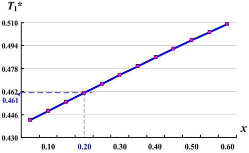
Moreover, Figure 8 depicts the impact of random scrap rate x on E[TCU(T₁*)]. It reveals that as x goes up, the expected system cost E[TCU(T₁*)] increases significantly. At x ∈[0, 0.2] as assumed in our example, it confirms the optimal E[TCU(T₁*)] = $11,301.

Figure 8. Impact of random scrap rate x on E[TCU(T₁*)].

The effect of variations in mean-time-to-failure (MTTF) 1/β on E[TCU(T₁*)] is explored and its result is illustrated in Figure 9. It not only highlights the relationship between 1/β and E[TCU(T₁*)] (for instance, our optimal solution at 1/β = 2 and E[TCU(T₁*)] = $11,301), but also shows that as the MTTF grows up to 2 years or longer, the proposed model is converted into the same model but without the machine failure factor.

Figure 9. Effect of variations in mean-time-to-failure (MTTF) 1/β on E[TCU(T₁*)].

Extra analysis on the impact of random scrap rate x on optimal fabrication uptime T₁* is exposed in Figure 10. It shows that as x increases, optimal fabrication uptime gets longer accordingly.

4.2. Impacts of fabrication uptime and number of deliveries to the proposed system

Effect of variations in fabrication uptime T₁ on E[TRCU(T₁)] is analysed and exhibited in Figure 11. It reconfirms the convexity and the optimal solution of our numerical example (i.e. T₁* = 0.461 years and E[TCU(T₁*)] = $11,301).

Figure 10. Impact of random scrap rate x on T₁*.

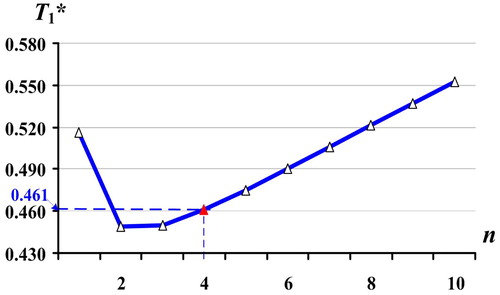
Further analysis on the impact of the number of deliveries per cycle n on E[TCU(T₁*)] and on T₁* are depicted in Figures 12 and 13, respectively. From Figure 12 it is noted that as number of deliveries per cycle n increases, E[TCU(T₁*)] rises notably.

Figure 11. Effect of variations in T on E[TCU(T₁)].

Figure 13 exposes the relationship between n and the optimal uptime T₁* and reconfirms our previous optimal solution (i.e. at n = 4, E[TCU(T₁*)] = $11,301).

4.3. Effect of the acceptable service-level constraint on the proposed system

Additional exploration on the impact of acceptable stock-out level (i.e. service-level) constraint on the proposed system is conducted and exhibited in Table 2. The effects of variations in service level (1 – α) on maximal holding and backlogging level, their related costs, E[TRCU(T₁*)] and the percentage increase in E[TRCU(T₁*)] are disclosed for managerial decision makings. For example, it indicates that with a system cost increase of 3.97%, we can bring the service level up to 80% (and of course this result is based on unit backlogging cost b = 0.1 as assumed in our numerical example).

Table 2. Effects of various service-level percentages on diverse system parameters/costs.

Service level (1 – α)%	Maximal stock holding level H	Maximal backlogging level B	Annual holding cost	Annual backordering cost	E[TCU(T1*)]	Percentage increase in E[TCU(T1*)]
100%	3509	0	$1,255	$0	$11,737	7.99
95%	3495	180	$1,197	$0	$11,620	6.91
90%	3472	378	$1,140	$2	$11,507	5.88
85%	3439	594	$1,084	$4	$11,401	4.89
80%	3391	830	$1,031	$8	$11,301	3.97
75%	3327	1085	$980	$14	$11,208	3.12
70%	3242	1359	$931	$20	$11,124	2.35
65%	3133	1648	$886	$29	$11,050	1.67
60%	2997	1950	$845	$39	$10,987	1.09
55%	2831	2257	$808	$51	$10,937	0.62
50%	2635	2563	$777	$64	$10,899	0.28
45%	2410	2858	$751	$79	$10,876	0.07
39%	2108	3184	$729	$97	$10,869	–

The effect of variations in service-level constraint (1 – α) on E[TCU(T₁*)] is investigated and illustrated in Figure 14. It shows that as we set service level (1 – α) higher, the expected system cost E[TCU(T₁*)] increases accordingly; it also reconfirms our optimal solution at (1 – α)% = 80%.

Figure 13. Impact of number of deliveries per cycle n on T₁*.

Finally, we demonstrate that this exact model can also provide production managers with joint impacts of combined system factors on the proposed system. For instance, the joint impacts of service-level constraint (1 – α) and MTTF (1/β) on E[TCU(T₁*)] are explored and exhibited in Figure 15. It is noted that as (1 – α) is set higher, E[TCU(T₁*)] increases drastically; and as MTTF becomes longer, 0.5 and up, E[TCU(T₁*)] declines notably.

Figure 14. Effect of variations in service level constraint (1 – α) on E[TCU(T₁)].

Figure 15. Joint impacts of service-level constraint (1 – α) and 1/β on E[TCU(T₁*)].

Figure A-1. The on-hand scrap level at time t in the proposed system with no breakdown happening in uptime.

4.4. Comparison of the obtained result with that in existing works

The obtained result is compared to existing works as follows: (i) if “service-level constraint” is not considered in this study, then E[TRCU(T₁*)] = $10,869 (Table 2 and Ting et al., 2011); (ii) if “stochastic breakdown rate” is not considered in the proposed study (Chiu, 2006; Chiu et al., 2007), then E[TRCU(T₁*)] = $11,197. In summary, without such an in-depth exploration, diverse key system characteristics such as the effect and joint effect of individual/combined factor(s) of stochastic machine failures, product quality, service-level constraints and number of deliveries on the proposed problem will remain inaccessible to the production decision-makers.

5. Concluding remarks

A fabrication–inventory problem that considers the production of scrap items, an acceptable level of stock outs with backordering, stochastic machine failures, and a multi-shipment policy is explored in this study. Further, a mathematical model is built to accurately portray the problem. Furthermore, an optimization method, along with an algorithm is presented to derive optimal fabrication uptime that minimizes total system costs.

This precise model and its solution process can not only provide an optimal uptime decision, but also reveals diverse and valuable system characteristics, such as the (1) details of cost components of the system (Figure 7); (2) effects of relevant quality factors (Figures 8–10); (3) impact of uptime and number of deliveries (Figures 11–13); (4) the effect of service-level constraints (Figure 14); and (5) joint impact of combined system factors (Figure 15) on the proposed system. The study contributes to existing literature by enabling production managers to comprehend the individual and joint impact of system factors on the practical fabrication–inventory problem. In addition, the result helps managers to answer realistic questions about production planning and control, such as (i) to what extent will the scrap and/or machine failure rates affect total system costs?; (ii) how much will it cost to bring the service level up to a desired level?; and (iii) what will be the effect on total system costs if a different number is chosen for deliveries per cycle? Finally, it suggests that an important topic that future study can examine is the effect of variable demand rate on the fabrication–inventory problem.

Figure 12. Impact of number of deliveries per cycle n on E[TCU(T₁*)].

Figure A-2. The on-hand finished product level in distribution time t₂′ in the proposed system with no breakdown happening in uptime.

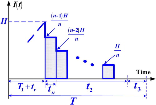
Table B-1. Results of convexity test for E[TCU(T₁)] by using extra values of β.

β	T1U	Equation (30)*(30) $$\frac{2\left(z_1+\frac{n{K}_1}{P}+w_1+w_3{e}^{-\beta T_1}+\frac{w_5}{n}+\frac{w_7{e}^{-\beta T_1}}{n}\right)+z_0\left(1-e^{-\beta T_1}\right)}{\left(\begin{array}{c}-T_1{}^2{\beta }^2{w}_2{e}^{-\beta T_1}-T_1{\beta }^2{w}_3{e}^{-\beta T_1}-2\beta w_3{e}^{-\beta T_1}-T_1{}^2{\beta }^2{s}^2{w}_4{e}^{-\beta T_{1}s}-\frac{T_1{}^2{\beta }^2{w}_6{e}^{-\beta T_1}}{n}\\ -\frac{T_1{\beta }^2{w}_7{e}^{-\beta T_1}}{n}-\frac{2\beta w_7{e}^{-\beta T_1}}{n}-T_1\beta e^{-\beta T_1}{z}_0-T_1{}^2\beta e^{-\beta T_1}\left(\frac{h_3\lambda g}{P}\right)\end{array}\right)}>T_1>0$$(30)	T1L	z(T1L)**
5.00	0.560	3.516	0.259	1.101
4.00	0.561	2.810	0.286	1.207
3.00	0.563	2.398	0.317	1.358
2.00	0.567	2.276	0.354	1.619
1.00	0.580	2.687	0.397	2.270
0.50	0.604	3.602	0.421	3.224
:	:	:	:	:
0.01	1.778	11.790	0.447	7.450

* Denotes the computation result from the left-hand side of Equation (30)(30) $$\frac{2\left(z_1+\frac{n{K}_1}{P}+w_1+w_3{e}^{-\beta T_1}+\frac{w_5}{n}+\frac{w_7{e}^{-\beta T_1}}{n}\right)+z_0\left(1-e^{-\beta T_1}\right)}{\left(\begin{array}{c}-T_1{}^2{\beta }^2{w}_2{e}^{-\beta T_1}-T_1{\beta }^2{w}_3{e}^{-\beta T_1}-2\beta w_3{e}^{-\beta T_1}-T_1{}^2{\beta }^2{s}^2{w}_4{e}^{-\beta T_{1}s}-\frac{T_1{}^2{\beta }^2{w}_6{e}^{-\beta T_1}}{n}\\ -\frac{T_1{\beta }^2{w}_7{e}^{-\beta T_1}}{n}-\frac{2\beta w_7{e}^{-\beta T_1}}{n}-T_1\beta e^{-\beta T_1}{z}_0-T_1{}^2\beta e^{-\beta T_1}\left(\frac{h_3\lambda g}{P}\right)\end{array}\right)}>T_1>0$$(30) with T_1U.

** Stands for the computation result from the left-hand side of Equation (30)(30) $$\frac{2\left(z_1+\frac{n{K}_1}{P}+w_1+w_3{e}^{-\beta T_1}+\frac{w_5}{n}+\frac{w_7{e}^{-\beta T_1}}{n}\right)+z_0\left(1-e^{-\beta T_1}\right)}{\left(\begin{array}{c}-T_1{}^2{\beta }^2{w}_2{e}^{-\beta T_1}-T_1{\beta }^2{w}_3{e}^{-\beta T_1}-2\beta w_3{e}^{-\beta T_1}-T_1{}^2{\beta }^2{s}^2{w}_4{e}^{-\beta T_{1}s}-\frac{T_1{}^2{\beta }^2{w}_6{e}^{-\beta T_1}}{n}\\ -\frac{T_1{\beta }^2{w}_7{e}^{-\beta T_1}}{n}-\frac{2\beta w_7{e}^{-\beta T_1}}{n}-T_1\beta e^{-\beta T_1}{z}_0-T_1{}^2\beta e^{-\beta T_1}\left(\frac{h_3\lambda g}{P}\right)\end{array}\right)}>T_1>0$$(30) with T_1L.

Acknowledgement

Authors express gratitude to the Ministry of Science and Technology of Taiwan for sponsoring this study (under grant no.#: MOST 103-2410-H-324-006-MY2).

Disclosure statement

No potential conflict of interest was reported by the authors.

Additional information

Funding

This work was supported by the Ministry of Science and Technology of Taiwan under Grant number: MOST 103-2410-H-324-006-MY2.

Appendix A

Additional illustrations and the basic formulas for analysing condition 3 – when no breakdown happens during uptime T₁ (A-1) $$t_4=\frac{B}{\left(P_1-d_1\right)}$$(A-1) (A-2) $$t_3=\frac{B-\lambda t_4}{\lambda }$$(A-2) (A-3) $$T_1=\left(t_4+t_1\right)=\frac{Q}{P_1}$$(A-3) (A-4) $$t_1=\frac{H}{\left(P_1-d_1\right)}$$(A-4) (A-5) $$H=\left(P_1-d_1\right)t_1$$(A-5) (A-6) $$T=\sum _{i=1}^4{t}_i$$(A-6) (A-7) $$t_2=T-\left(t_1+t_3+t_4\right)$$(A-7) (A-8) $$d_1{T}_1=xQ$$(A-8) (A-9) $$t_n=\frac{t_2}{n}$$(A-9) (A-10) $$\left(\frac{1}{n^2}\right)\left(\sum _{i=1}^{n-1}i\right)H{t}_2=\left(\frac{n-1}{2n}\right)H{t}_2$$(A-10)

Appendix B

Extra β values are applied to convexity test for E[TCU(T₁)] and the analytical results as shown in the following Table B – 1 so as to demonstrate the applicability of the proposed system. It reveals that the proposed model is good for solving the specific problems with wide-ranging failure rates.

References

- Abboud, N. E. (2001). Discrete-time Markov production–inventory model with machine breakdowns. Computers and Industrial Engineering, 39(1-2), 95–107. doi: 10.1016/S0360-8352(00)00070-X
- Abilash, N., & Sivapragash, M. (2016). Optimizing the delamination failure in bamboo fiber reinforced polyester composite. Journal of King Saud University - Engineering Sciences, 28(1), 92–102. doi: 10.1016/j.jksues.2013.09.004
- Abubakar, M., Basheer, U., & Ahmad, N. (2017). Mesoporosity, thermochemical and probabilistic failure analysis of fired locally sourced kaolinitic clay. Journal of the Association of Arab Universities for Basic and Applied Sciences, 24(1), 81–88. doi: 10.1016/j.jaubas.2017.04.002
- Afshar-Nadjafi, B., & Afshar-Nadjafi, A. (2017). A constructive heuristic for time-dependent multi-depot vehicle routing problem with time-windows and heterogeneous fleet. Journal of King Saud University - Engineering Sciences, 29(1), 29–34. doi: 10.1016/j.jksues.2014.04.007
- Archetti, C., Doerner, K. F., & Tricoire, F. (2013). A heuristic algorithm for the free newspaper delivery problem. European Journal of Operational Research, 230(2), 245–257. doi: 10.1016/j.ejor.2013.04.039
- Balaji, M., Velmurugan, V., Prapa, M., & Mythily, V. (2016). A fuzzy approach for modeling and design of agile supply chains using interpretive structural modeling. Jordan Journal of Mechanical and Industrial Engineering, 10(1), 67–74.
- Banerjee, A. (1986). A joint economic-lot-size model for purchaser and vendor. Decision Sciences, 17(3), 292–311. doi: 10.1111/j.1540-5915.1986.tb00228.x
- Bashyam, S., & Fu, M. C. (1998). Optimization of (s, S) inventory systems with random lead times and a service level constraint. Management Science, 44(12-part-2), S243–S256. doi: 10.1287/mnsc.44.12.S243
- Buscher, U., & Lindner, G. (2005). Optimizing a production system with rework and equal sized batch shipments. Computers & Operations Research, 32, 515–535. doi: 10.1016/j.cor.2005.03.011
- Caiazza, R., Volpe, T., & Stanton, J. L. (2016). Global supply chain: The consolidators' role. Operations Research Perspectives, 3, 1–4. doi: 10.1016/j.orp.2015.10.001
- Cardós, M., Babiloni, E., Palmer, M. E., & Guijarro, E. (2013). A heuristic to minimize the inventory value of repairable parts with service constraints: Application to an airline company. Journal of Industrial Engineering and Management, 6(3 SPL.ISS), 771–778.
- Chakraborty, T., Giri, B. C., & Chaudhuri, K. S. (2008). Production lot sizing with process deterioration and machine breakdown. European Journal of Operational Research, 185(2), 606–618. doi: 10.1016/j.ejor.2007.01.011
- Chiu, Y.-S. P. (2006). The effect of service level constraint on EPQ model with random defective rate. Mathematical Problems in Engineering, 2006 art. ID 98502, 1–13. doi: 10.1155/MPE/2006/98502
- Chiu, Y.-S. P., Ting, C.-K., Cheng, C.-B., & Lin, F.-Y. (2007). Alternative approach for realistic lot-size problem with random scrap rate and backlogging. WSEAS Transactions on Mathematics, 6(6), 736–740.
- Chiu, Y.-S. P., Hsieh, Y.-T., Kuo, J.-S., & Chiu, S. W. (2016). A delayed differentiation multi-product FPR model with scrap and a multi-delivery policy – I: Using single-machine production scheme. International Journal for Engineering Modelling, 29(1-4), 37–52.
- Chiu, S. W., Liu, C.-J., Li, Y.-Y., & Chou, C.-L. (2017). Manufacturing lot size and product distribution problem with rework, outsourcing and discontinuous inventory distribution policy. International Journal for Engineering Modelling, 30(1-4), 49–61.
- de Kok, A. G. (1985). Approximation for a lost-sales production/inventory control model with service level constraints. Management Science, 31(6), 729–737. doi: 10.1287/mnsc.31.6.729
- Florea Ionescu, A. I., Corboş, R.-A., Popescu, R. I., & Zamfir, A. (2016). From the factory floor to the shop floor – improved supply chain for sustainable competitive advantage with item-level RFID in retail. Economic Computation and Economic Cybernetics Studies and Research, 50(4), 119–134.
- Gopinath, S. C. B., Lakshmipriya, T., Md Arshad, M. K., Voon, C. H., Adam, T., Hashim, U., … Chinni, S. V. (2017). Shortening full-length aptamer by crawling base deletion – Assisted by Mfold web server application. Journal of the Association of Arab Universities for Basic and Applied Sciences, 23(1), 37–42. doi: 10.1016/j.jaubas.2016.07.001
- Groenevelt, H., Pintelon, L., & Seidmann, A. (1992). Production lot sizing with machine breakdowns. Management Sciences, 38(1), 104–123. doi: 10.1287/mnsc.38.1.104
- Hall, R. W. (1996). On the integration of production and distribution: economic order and production quantity implications. Transportation Research Part B: Methodological, 30(5), 387–403. doi: 10.1016/0191-2615(96)00002-1
- Jaber, M. Y. (2006). Lot sizing for an imperfect production process with quality corrective interruptions and improvements, and reduction in setups. Computers & Industrial Engineering, 51(4), 781–790. doi: 10.1016/j.cie.2006.09.001
- Jaggi, C. K., Khanna, A. & Nidhi, (2016). Effects of inflation and time value of money on an inventory system with deteriorating items and partially backlogged shortages. International Journal of Industrial Engineering Computations, 7(2), 267–282. doi: 10.5267/j.ijiec.2015.10.003
- Jawla, P., & Singh, S. R. (2016). Multi-item economic production quantity model for imperfect items with multiple production setups and rework under the effect of preservation technology and learning environment. International Journal of Industrial Engineering Computations, 7(4), 703–716. doi: 10.5267/j.ijiec.2016.2.003
- Jindal, P., & Solanki, A. (2016). Integrated supply chain inventory model with quality improvement involving controllable lead time and backorder price discount. International Journal of Industrial Engineering Computations, 7(3), 463–480. doi: 10.5267/j.ijiec.2015.12.003
- Khalili, A., Ismail, M. Y., Karim, A. N. M., & Che Daud, M. R. (2017). Critical success factors for soft AQM and lean manufacturing linkage. Jordan Journal of Mechanical and Industrial Engineering, 11(2), 129–140.
- Khan, M., Jaber, M. Y., & Ahmad, A.-R. (2014). An integrated supply chain model with errors in quality inspection and learning in production. Omega, 42(1), 16–24. doi: 10.1016/j.omega.2013.02.002
- Kim, C. H., & Hong, Y. (1997). An extended EMQ model for a failure prone machine with general lifetime distribution. International Journal of Production Economics, 49(3), 215–223. doi: 10.1016/S0925-5273(97)00013-3
- Lee, H., & Rosenblatt, M. (1987). Simultaneous determination of production cycle and inspection schedules in a production system. Management Science, 33(9), 1125–1136. doi: 10.1287/mnsc.33.9.1125
- Liu, L., Liu, X., Wang, X., Wang, Y., & Li, C. (2017). Reliability analysis and evaluation of a brake system based on competing risks. Journal of Engineering Research, 5(3), 150–161.
- Mičieta, B., Herčko, J., Botka, M., & Zrnić, N. (2016). Concept of intelligent logistic for automotive industry. Istrazivanja i Projektovanja za Privredu, 14(2), 233–238. doi: 10.5937/jaes14-10907
- MohanDas, C. D., Ayyanar, A., Susaiyappan, S., & Kalimuthu, R. (2017). Analysis of the effects of fabrication parameters on the mechanical properties of Areca fine fiber-reinforced phenol formaldehyde composite using Taguchi technique. Journal of Applied Research and Technology, 15(4), 365–370. doi: 10.1016/j.jart.2017.03.003
- Moinzadeh, K., & Aggarwal, P. (1997). Analysis of a production/inventory system subject to random disruptions. Management Science, 43(11), 1577–1588. doi: 10.1287/mnsc.43.11.1577
- Oblak, L., Kuzman, M. K., & Grošelj, P. (2017). A fuzzy logic-based model for analysis and evaluation of services in a Manufacturing company. Istrazivanja i Projektovanja za Privredu, 15(3), 258–271. doi: 10.5937/jaes15-13399
- Raj, V., & Prabha, G. (2016). Synthesis, characterization and in vitro drug release of cisplatin loaded Cassava starch acetate – PEG/gelatin nanocomposites. Journal of the Association of Arab Universities for Basic and Applied Sciences, 21(1), 10–16. doi: 10.1016/j.jaubas.2015.08.001
- Rakyta, M., Fusko, M., Herčko, J., Závodská, L., & Zrnić, N. (2016). Proactive approach to smart maintenance and logistics as a auxiliary and service processes in a company. Istrazivanja i Projektovanja za Privredu, 14(4), 433–442. doi: 10.5937/jaes14-11664
- Razmi, J., Kazerooni, M. P., & Sangari, M. S. (2016). Designing an integrated multi-echelon, multi-product and multi-period supply chain network with seasonal raw materials. Economic Computation and Economic Cybernetics Studies and Research, 50(1), 273–290.
- Rivera-Gómez, H., Gharbi, A., & Kenné, J. P. (2013). Production and quality control policies for deteriorating manufacturing system. International Journal of Production Research, 51(11), 3443–3462. doi: 10.1080/00207543.2013.774494
- Salemi, H. (2016). A hybrid algorithm for stochastic single-source capacitated facility location problem with service level requirements. International Journal of Industrial Engineering Computations, 7(2), 295–308. doi: 10.5267/j.ijiec.2015.10.001
- Schwarz, L. B. (1973). A simple continuous review deterministic one-warehouse N-retailer inventory problem. Management Science, 19(5), 555–566. doi: 10.1287/mnsc.19.5.555
- Selçuk, B., & Ağralı, S. (2013). Joint spare parts inventory and reliability decisions under a service constraint. Journal of the Operational Research Society, 64(3), 446–458. doi: 10.1057/jors.2012.38
- Settanni, E., Harrington, T. S., & Srai, J. S. (2017). Pharmaceutical supply chain models: A synthesis from a systems view of operations research. Operations Research Perspectives, 4, 74–95. doi: 10.1016/j.orp.2017.05.002
- Taft, E. W. (1918). The most economical production lot. Iron Age, 101, 1410–1412.
- Tempelmeier, H. (2007). On the stochastic uncapacitated dynamic single-item lotsizing problem with service level constraints. European Journal of Operational Research, 181(1), 184–194. doi: 10.1016/j.ejor.2006.06.009
- Ting, C.-K., Chiu, Y.-S. P., & Chan, C.-C. H. (2011). Optimal lot sizing with scrap and random breakdown occurring in backorder replenishing period. Mathematical and Computational Applications, 16(2), 329–339. doi: 10.3390/mca16020329
- Zahedi, Z., Ari Samadhi, T. M. A., Suprayogi, S., & Halim, A. H. (2016). Integrated batch production and maintenance scheduling for multiple items processed on a deteriorating machine to minimize total production and maintenance costs with due date constraint. International Journal of Industrial Engineering Computations, 7(2), 229–244. doi: 10.5267/j.ijiec.2015.10.006