Variable thermal conductivity approach for bioheat transfer during thermal ablation

Abstract

The aim of the article is to present a mathematical model that predicts tissue temperature during thermal therapy (thermal ablation). The mathematical formulation of variable thermal conductivity of thermal wave bioheat transfer model for a generalized coordinate system due to external heat source during thermal ablation has been given. The governing bioheat transfer equation is simplified by Kirchhoff’s transformation. The numerical solution of the problem has been achieved using a finite difference scheme to discretize in space coordinate; the reduced system of second order ordinary differential equation is solved by the finite element Legendre wavelet Galerkin method (FELWGM). The obtained result from FELWGM is compared with exact analytical solution and shows good agreement. Parametric study is performed to evaluate the effect of variable thermal conductivity on tissue temperature distribution for different physical parameters and illustrated graphically. Particular cases are also deduced from present investigation. The effect of variability of thermal conductivity parameter, variability of time, generalized coordinate system, lagging time and external heat source coefficient on tissue temperature is discussed in detail. Thus, the consideration of the variable thermal conductivity is extremely beneficial for the clinical therapeutic application in the treatment of cancerous cells.

Keywords:

• Bioheat transfer
• thermal ablation
• Kirchhoff’s transformation
• finite element Legendre wavelet Galerkin method
• variable thermal conductivity
• lagging time

1. Introduction

For image-guided thermal treatments delivering of heat via focused ultrasound (FUS), radiofrequency (RF), microwave (MW), or laser, temperature induced changes in tissue properties are of relevance in relation to predicting tissue temperature profile, monitoring during treatment, and evaluation of treatment results. These thermal treatments cause reversible or irreversible changes in the properties of tissues. Therefore, for thermal therapies the adequate consideration of tissue properties and their temperature dependence is necessary to achieve accurate results.

Mathematical modelling of thermal therapies has been used extensively to predict and optimize clinical treatments and medical devices. Pennes (1948) model is widely used to model such problems. Kumar, Kumar, and Rai (2015a) studied the heat transfer process in biological tissue during thermal ablation in a generalized coordinate system. Non-linear dual-phase-lag model is utilized by Kumar, Kumar, and Rai (2016) in living tissue during thermal ablation. Kumar and Rai (2017) studied the time fractional DPL model in presence of temperature dependent metabolic and electromagnetic radiation heat source. Kashcooli, Salimpour, and Shirani (2017) investigated the effects of blood vessels on temperature distribution in a skin tissue subjected to various thermal therapy conditions.

Recently, Kumar, Damor, and Shukla, (2018) studied the heat transfer thermal damage in triple layer skin tissue using a fractional bioheat model. For therapeutic treatment of cancerous cells, Kumar, Singh, Sharma, and Rai (2018) used non-linear dual-phase-lag model under Dirichlet boundary conditions. Tan, Zou, Dong, Ding, and Zhao (2018) investigated the coupled effects of blood vessels and relaxation time on tissue temperature and thermal lesion region during HIFU hyperthermia.

Very few authors considered the temperature-dependent thermal parameters over wide temperature ranges in tissues. Valvano, Cochran, and Diller (1985) measured thermal conductivity and diffusivity of biomaterials over a wide temperature range. Bhattacharya and Mahajan (2003) presented the temperature-dependent thermal conductivity of sheep collagen and cow liver in vitro. Watanabe, Kobayashi, Hashiszume, and Fujie (2009) investigated the effects of the temperature dependence of thermophysical properties of the liver on the temperature distribution during RFA. Trujillo and Berjano (2013) reviewed the mathematical functions most commonly used for modelling the temperature dependence of electrical and thermal conductivities of biological tissue in RFA.

Guntur, Lee, Paeng, Coleman, and Choi (2013) found that the thermal properties of ex vivo porcine liver tissue during RFA vary significantly with temperature. Rossmann and Haemmerich (2014) reviewed temperature-dependent thermal and electrical properties of biological tissues in the supraphysiological temperature regime. Guntur and Choi (2015) examined the effects of temperature-dependent thermal parameters on the temperature distribution in liver tissue exposed to a clinical high-intensity focused ultrasound (HIFU) field, and found that alteration of tissue thermal parameters significantly affects the prediction of temperature distributions and suggest that the dependence of thermal parameters should be considered in estimation of the thermal dose in tissues exposed to a clinical HIFU field.

Very useful work has been carried out by Ellahi et al. on thermal conductivity; notable among them are Bhatti, Zeeshan, and Ellahi (2017), Bhatti, Zeeshan, Ellahi, and Shit (2018), Bhatti, Zeeshan, Tripathi, and Ellahi (2018), Ellahi, Alamri, Sultan, Basit, and Majeed, (2018), Ellahi, Zeeshan, Shehzad, and Alamri (2018), Hassan, Marin, Ellahi, and Alamri (2018), Ijaz, Zeeshan, Bhatti, and Ellahi (2018). Akbar, Raza, and Ellahi (2016a) studied the effects of entropy and magnetic field in an endoscope for a thermal conductivity model. Akbar, Raza, and Ellahi (2016b) studied the anti-bacterial applications for new thermal conductivity model in arteries with CNT suspended nanofluid.

The present study aims to investigate the effects of variable thermal conductivity during thermal ablation for a thermal wave bioheat transfer model with modified Gaussian external heat source in a generalized coordinate system. The governing bioheat transfer equation is simplified by Kirchhoff’s transformation and then finite difference scheme, and Legendre wavelet Galerkin approach is used to solve the problem. The problem is converted into a system of second order differential equation with initial conditions by using the finite difference scheme in space coordinate. Then, this reduced system is solved by the Wavelet Galerkin approach with Legendre wavelet as basis function, which reduces the problem into the Sylvester matrix equation. The solution of the Sylvester matrix equation gives the temperature distribution during thermal ablation with variable thermal conductivity and a significant effect of the variable conductivity has been observed on tissue temperature distribution.

2. Formulation of the problem

Consider a tissue of finite length (L), which is heated by modified Gaussian external heat source with variable thermal conductivity during thermal ablation in generalized coordinate system. Pennes (1948) performed a series of experiments that measured temperatures on human forearms and derived a thermal energy conservation equation known as bioheat transfer equation as follows:

From the principle of conservation of energy to tissue control volume (V), we have (1) $$U_{\text{gain}}=U_{\text{storage}}+U_{\text{loss}},$$(1)

where U_gain, U_storage, and U_loss are given below.

The general internal heat generation per unit volume due to metabolic heat (q_m) and the interior heat caused by outer heat source (q_s) is (2) $$U_{\text{gain}}={\int }_V(q_{\mathrm{m}}+q_{\mathrm{s}})\mathrm{d}V={\int }_V{q}_{\mathrm{t}}(x,t)\mathrm{d}V.$$(2)

The total rate of stored thermal energy over the control volume is (3) $$U_{\text{storage}}={\int }_V\rho c\frac{\partial T(x,t)}{\partial t}\mathrm{d}V.$$(3)

Heat loss to adjacent tissues by convection and conduction is given as (4) $$U_{\text{loss}}=U_{\mathrm{c}}-U_{\mathrm{b}},$$(4)

where (5) $$U_{\mathrm{c}}={\int }_{A}q.ndA,$$(5)

is the rate production through the control volume and (6) $$U_{\mathrm{b}}={\int }_V{q}_{\mathrm{b}}\mathrm{d}V,$$(6)

the total amount of thermal energy over the tissue control volume.

Using Equations (2)–(6) in Equation (1)(1) $$U_{\text{gain}}=U_{\text{storage}}+U_{\text{loss}},$$(1) , yields (7) $${\int }_V{q}_{\mathrm{t}}(x,t)\mathrm{d}V={\int }_V\rho c\frac{\partial T(x,t)}{\partial t}\mathrm{d}V+{\int }_{A}q.ndA-{\int }_V{q}_b\mathrm{d}V.$$(7)

Applying the divergence theorem to the surface integral and observing that Equation (7)(7) $${\int }_V{q}_{\mathrm{t}}(x,t)\mathrm{d}V={\int }_V\rho c\frac{\partial T(x,t)}{\partial t}\mathrm{d}V+{\int }_{A}q.ndA-{\int }_V{q}_b\mathrm{d}V.$$(7) must hold for any arbitrary volume element, we obtain (8) $$\rho c\frac{\partial T}{\partial t}-q_{\mathrm{b}}-q_{\mathrm{m}}-q_{\mathrm{s}}=-\frac{\partial q}{\partial r}.$$(8)

Cattaneo (1958), Vernotte (1958) proposed the following modified heat flux model that is a linear extension of the Fourier’s law in order to take in the wave-like behaviour in heat conduction process, (9) $$\left(1+{\tau }_q\frac{\partial }{\partial t}\right)q=-k\left(T\right)\frac{\partial T}{\partial r},$$(9)

where k(T) is the thermal conductivity with variable temperature.

Using Equation (9)(9) $$\left(1+{\tau }_q\frac{\partial }{\partial t}\right)q=-k\left(T\right)\frac{\partial T}{\partial r},$$(9) in Equation (8)(8) $$\rho c\frac{\partial T}{\partial t}-q_{\mathrm{b}}-q_{\mathrm{m}}-q_{\mathrm{s}}=-\frac{\partial q}{\partial r}.$$(8) with temperature dependent specific heat yields (10) $$\left(1+{\tau }_q\frac{\partial }{\partial t}\right)\left(\rho c\left(T\right)\frac{\partial T}{\partial t}-q_{\mathrm{b}}-q_{\mathrm{m}}-q_{\mathrm{s}}\right)=\frac{\partial }{\partial r}\left(k\left(T\right)\frac{\partial T\left(r,t\right)}{\partial t}\right).$$(10)

Equation (10)(10) $$\left(1+{\tau }_q\frac{\partial }{\partial t}\right)\left(\rho c\left(T\right)\frac{\partial T}{\partial t}-q_{\mathrm{b}}-q_{\mathrm{m}}-q_{\mathrm{s}}\right)=\frac{\partial }{\partial r}\left(k\left(T\right)\frac{\partial T\left(r,t\right)}{\partial t}\right).$$(10) in generalized coordinate system can be written as (11) $$\left(1+{\tau }_q\frac{\partial }{\partial t}\right)\left(\frac{k\left(T\right)}{\kappa }\frac{\partial T}{\partial t}-q_{\mathrm{b}}-q_{\mathrm{m}}-q_{\mathrm{s}}\right)=\frac{1}{r^{\Gamma }}\frac{\partial }{\partial r}\left(r^{\Gamma }k\left(T\right)\frac{\partial T}{\partial t}\left(r,t\right)\right),0<r<L,t>0,$$(11)

where $\Gamma =0,1,2$ corresponds to Cartesian, axis-symmetric, and spherical symmetric coordinate system and (12) $$\rho c\left(T\right)=\frac{k\left(T\right)}{\kappa }.$$(12)

The term q_b can be expressed as (13) $$q_{\mathrm{b}}={\omega }_{\mathrm{b}}{\rho }_{\mathrm{b}}{c}_{\mathrm{b}}\left(T_{\mathrm{a}}-T\right).$$(13)

The term q_m can be approximated as a linear function of local tissue temperature taken in Gupta, Singh, and Rai (2010), (14) $$q_{\mathrm{m}}=q_{\mathrm{m}0}\left(1+\frac{T-T_0}{T_0}\right),$$(14)

Following (Kumar, Kumar, & Rai, 2015b) modified Gaussian heat source q_s is taken as (15) $$q_{\mathrm{s}}\left(r,t\right)=\rho SP{\mathrm{e}}^{-a_0^2{\left(r-r_0\right)}^2}.$$(15)

To solve the problem, the following initial and boundary conditions are taken:

Initial conditions (16) $$T(r,0)=T_0\text{and}\frac{\partial T(r,0)}{\partial t}=0,$$(16)

Boundary conditions (17) $$T(0,t)=T_w,$$(17)

Symmetric condition (18) $$\frac{\partial T(L,t)}{\partial r}=0.$$(18)

Considering the mapping (Kirchhoff’s transformation), following Hetnarski (1986) as (19) $$\vartheta =\frac{1}{k_0}{\int }_0^{T}k(\xi )d\xi ,$$(19)

yields (20) $$k_0\frac{\partial \vartheta }{\partial r}=k\left(T\right)\frac{\partial T}{\partial r},k_0\frac{{\partial }^2\vartheta }{\partial r^2}=\frac{\partial }{\partial r}\left(k\left(T\right)\frac{\partial T}{\partial r}\right),k_0\frac{\partial \vartheta }{\partial t}=k\left(T\right)\frac{\partial T}{\partial t}.$$(20)

An important factor to achieve realistic models is the use of mathematical functions to describe the temperature dependence of thermal properties of tissue. A commonly used approach for modelling the temperature dependence of thermal properties for temperature below ${100}^{°}\mathrm{C}$ is based on linear equations and employs constant temperature coefficient such as: (21) $$k\left(T\right)=k_0\left(1+k_{1}T\right).$$(21)

From the above, we have the following relations: (22) $$\vartheta =T+\frac{k_1}{2}{T}^2,\frac{\partial \vartheta }{\partial r}=\frac{\partial T}{\partial r}\left(1+k_{1}T\right),\frac{\partial \vartheta }{\partial t}=\frac{\partial T}{\partial t}\left(1+k_{1}T\right),$$(22)

and (23) $$T=\frac{-1+\sqrt{1+2k_1\vartheta }}{k_1}.$$(23)

Equations (11)(11) $$\left(1+{\tau }_q\frac{\partial }{\partial t}\right)\left(\frac{k\left(T\right)}{\kappa }\frac{\partial T}{\partial t}-q_{\mathrm{b}}-q_{\mathrm{m}}-q_{\mathrm{s}}\right)=\frac{1}{r^{\Gamma }}\frac{\partial }{\partial r}\left(r^{\Gamma }k\left(T\right)\frac{\partial T}{\partial t}\left(r,t\right)\right),0<r<L,t>0,$$(11) and (16–18) with the aid of Equations (19–21) in linear form become (24) $$\left(1+{\tau }_q\frac{\partial }{\partial t}\right)\left[\frac{k_0}{\kappa }\frac{\partial \vartheta }{\partial t}-q_{\mathrm{b}}-q_{\mathrm{m}}-q_{\mathrm{s}}\right]=k_0\frac{{\partial }^2\vartheta }{\partial r^2}+\frac{\Gamma }{r}{k}_0\frac{\partial \vartheta }{\partial t},$$(24)

(25) $$\vartheta \left(r,0\right)=T_0+\frac{k_1}{2}{T}_0^2,\frac{\partial \vartheta }{\partial r}\left(r,0\right)=0,$$(25) (26) $$\vartheta \left(0,t\right)=T_w+\frac{k_1}{2}{T}_w^2,\frac{\partial \vartheta }{\partial r}\left(0,t\right)=0.$$(26)

3. Solution of the problem

Introducing the non-dimensional variable and similarity criteria (27) $$\begin{array}{l}x=\frac{r}{L},x^{*}=\frac{r_0}{L},F_0={\omega }_{0}t,\Theta =\frac{\vartheta -T_0}{T_0},\theta =\frac{T-T_0}{T_0},{\vartheta }_a=\frac{T_a-T_0}{T_0},{\vartheta }_w=\frac{T_w-T_0}{T_0},\hfill \\ K_1=k_1{T}_0,F_{0q}={\omega }_0{\tau }_q,a=a_{0}L,P_f=\sqrt{\frac{W_b{c}_b{L}^2}{k_0}},P_{m0}=\frac{q_{m0}{L}^2}{T_0{k}_0},P_{r0}=\frac{q_{r0}{L}^2}{T_0{k}_0},\hfill \\ W_b={\omega }_b{\rho }_b,{\omega }_0=\frac{k_0}{\rho c{L}^2},d=.1T_0.\hfill \end{array}$$(27)

With the help of Equation (27)(27) $$\begin{array}{l}x=\frac{r}{L},x^{*}=\frac{r_0}{L},F_0={\omega }_{0}t,\Theta =\frac{\vartheta -T_0}{T_0},\theta =\frac{T-T_0}{T_0},{\vartheta }_a=\frac{T_a-T_0}{T_0},{\vartheta }_w=\frac{T_w-T_0}{T_0},\hfill \\ K_1=k_1{T}_0,F_{0q}={\omega }_0{\tau }_q,a=a_{0}L,P_f=\sqrt{\frac{W_b{c}_b{L}^2}{k_0}},P_{m0}=\frac{q_{m0}{L}^2}{T_0{k}_0},P_{r0}=\frac{q_{r0}{L}^2}{T_0{k}_0},\hfill \\ W_b={\omega }_b{\rho }_b,{\omega }_0=\frac{k_0}{\rho c{L}^2},d=.1T_0.\hfill \end{array}$$(27) , Equations (24–26) reduce to the following form (28) $$F_{0q}\frac{{\partial }^2\Theta }{\partial F_0^2}+\left(1+F_{0q}{P}_f^2-F_{0q}{P}_{m0}d\right)\frac{\partial \Theta }{\partial F_0}-\left(P_{m0}d-P_f^2\right)\Theta =\frac{{\partial }^2\Theta }{\partial x^2}+\frac{\Gamma }{x}\frac{\partial \Theta }{\partial x}+P_f^2{\vartheta }_a+P_{m0}+P_{r0}{\mathrm{e}}^{-a^2{\left(x-x^{*}\right)}^2},$$(28)

(29) $$\Theta (x,0)=\frac{K_1}{2},\frac{\partial \Theta }{\partial F_0}(x,0)=0,$$(29) (30) $$\Theta (0,F_0)=V_w,$$(30) (31) $$\frac{\partial \Theta }{\partial x}(1,F_0)=0,$$(31)

where $V_w={\vartheta }_w+\frac{K_1}{2}{({\vartheta }_w+1)}^2$.

3.1. Finite difference scheme for spatial-discretization

The space coordinate domain [0,1] divided into n + 1 sub intervals of equal step length (h) i.e. $0=x_0<x_1<x_2<\dots <x_n<x_{n+1}=1$, where $x_{i+1}=x_i+h$. The first and second order derivatives are approximated by using central difference formula i.e. (32) $$\frac{\partial \Theta (x,F_0)}{\partial r}{|}_{x=x_i}=\frac{{\Theta }_{i+1}-{\Theta }_{i-1}}{2h},$$(32)

(33) $$\frac{{\partial }^2\Theta (x,F_0)}{\partial r^2}{|}_{x=x_i}=\frac{{\Theta }_{i+1}\left(F_0\right)-2{\Theta }_i\left(F_0\right)+{\Theta }_{i-1}\left(F_0\right)}{h^2},$$(33)

$1\le i\le n.$

Using this spatial discretization scheme, Equation (28)(28) $$F_{0q}\frac{{\partial }^2\Theta }{\partial F_0^2}+\left(1+F_{0q}{P}_f^2-F_{0q}{P}_{m0}d\right)\frac{\partial \Theta }{\partial F_0}-\left(P_{m0}d-P_f^2\right)\Theta =\frac{{\partial }^2\Theta }{\partial x^2}+\frac{\Gamma }{x}\frac{\partial \Theta }{\partial x}+P_f^2{\vartheta }_a+P_{m0}+P_{r0}{\mathrm{e}}^{-a^2{\left(x-x^{*}\right)}^2},$$(28) becomes (34) $$F_{0q}\frac{{\partial }^2{\Theta }_i}{\partial F_0^2}+\left(1+F_{0q}{P}_f^2-F_{0q}{P}_{m0}d\right)\frac{\partial {\Theta }_i}{\partial F_0}-\left(P_{m0}d-P_f^2\right){\Theta }_i=\frac{{\Theta }_{i+1}-2{\Theta }_i+{\Theta }_{i-1}}{h^2}+\frac{\Gamma }{x_i}\left(\frac{{\Theta }_{i+1}-{\Theta }_{i-1}}{2h}\right)+P_f^2{\vartheta }_a+P_{m0}+P_{r0}{\mathrm{e}}^{-a^2{\left(x_i-x^{*}\right)}^2},$$(34)

$1\le i\le n,F_0>0$, with initial condition (35) $${\Theta }_i\left(0\right)=\frac{K_1}{2},\frac{d{\Theta }_i\left(0\right)}{d{F}_0}=0,$$(35)

boundary condition (36) $${\Theta }_0\left(F_0\right)=V_w,{\Theta }_{n+1}=\frac{1}{21}[13{\Theta }_n+17{\Theta }_{n+1}-9{\Theta }_{n+1}].$$(36)

The Equation (34)(34) $$F_{0q}\frac{{\partial }^2{\Theta }_i}{\partial F_0^2}+\left(1+F_{0q}{P}_f^2-F_{0q}{P}_{m0}d\right)\frac{\partial {\Theta }_i}{\partial F_0}-\left(P_{m0}d-P_f^2\right){\Theta }_i=\frac{{\Theta }_{i+1}-2{\Theta }_i+{\Theta }_{i-1}}{h^2}+\frac{\Gamma }{x_i}\left(\frac{{\Theta }_{i+1}-{\Theta }_{i-1}}{2h}\right)+P_f^2{\vartheta }_a+P_{m0}+P_{r0}{\mathrm{e}}^{-a^2{\left(x_i-x^{*}\right)}^2},$$(34) is converted into a system of second order ordinary differential equation in vector matrix form as follows: (37) $$F_{0q}\frac{d^2\Theta }{d{F}_0^2}+\left(1+F_{0q}{P}_f^2-F_{0q}{P}_{m0}d\right)\frac{d\Theta }{d{F}_0}-\left(P_{m0}d-P_f^2\right)I\Theta -A\Theta =B,$$(37)

subjected to initial condition (38) $$\Theta \left(0\right)=\frac{K_1}{2},\text{and}\frac{d\Theta \left(0\right)}{d{F}_0}=0,$$(38)

where $n=2^{k-1}M$, I is the identity matrix of order n, A is a square matrix of order $2^{k-1}M\times 2^{k-1}M$; B, $\Theta (0)$, and $\frac{d\Theta (0)}{d{F}_0}$ are the column matrix of $2^{k-1}M\times 1$ which are given as follows $$\begin{array}{l}A=\frac{1}{h^2}\left[\begin{array}{ccccccccc}-2& 1+\frac{\Gamma h}{2x_1}& 0& 0& 0& \dots & 0& 0& 0\\ 1-\frac{\Gamma h}{2x_2}& -2& 1+\frac{\Gamma h}{2x_2}& 0& 0& \dots & 0& 0& 0\\ 0& 1-\frac{\Gamma h}{2x_3}& -2& 1+\frac{\Gamma h}{2x_3}& 0& \dots & 0& 0& 0\\ ⋮& ⋮& ⋮& ⋮& ⋮& \dots & ⋮& ⋮& ⋮\\ 0& 0& 0& 0& 0& \dots & 1-\frac{\Gamma h}{2x_{n-1}}& -2& 1+\frac{\Gamma h}{2x_{n-1}}\\ 0& 0& 0& 0& 0& \dots & \frac{-9}{21}(1+\frac{\Gamma h}{2x_n})& \frac{17}{21}(1+\frac{\Gamma h}{2x_n})+(1-\frac{\Gamma h}{2x_n})& -2+\frac{13}{21}(1+\frac{\Gamma h}{2x_n})\end{array}\right],\\ B={\left[\begin{array}{ccccccc}{V}_w(\frac{1}{h^2}-\frac{\Gamma }{2x_{1}h})+B_1& B_2& B_3& \dots & B_i& \dots & B_n\end{array}\right]}^T,\end{array}$$

where $$B_i=P_f^2{\Theta }_a+P_{m0}+P_{r0}{e}^{-a^2{(x_i-x^{*})}^2},i=1,2,\dots ,n.$$

$$\Theta \left(0\right)={\left[\begin{array}{cccccc}{\Theta }_1\left(0\right)& {\Theta }_2\left(0\right)& \dots & {\Theta }_i\left(0\right)& \dots & {\Theta }_n\left(0\right)\end{array}\right]}^T,$$

and $$\frac{d\Theta \left(0\right)}{d{F}_0}={\left[\begin{array}{cccccc}\frac{d{\Theta }_1\left(0\right)}{d{F}_0}& \frac{d{\Theta }_2\left(0\right)}{d{F}_0}& \dots & \frac{d{\Theta }_i\left(0\right)}{d{F}_0}& \dots & \frac{d{\Theta }_n\left(0\right)}{d{F}_0}\end{array}\right]}^T.$$

3.2. Legendre wavelet Galerkin approach

To solve the differential Equation (37)(37) $$F_{0q}\frac{d^2\Theta }{d{F}_0^2}+\left(1+F_{0q}{P}_f^2-F_{0q}{P}_{m0}d\right)\frac{d\Theta }{d{F}_0}-\left(P_{m0}d-P_f^2\right)I\Theta -A\Theta =B,$$(37) , let us assume that (39) $$\frac{d^2\Theta }{d{F}_0^2}={\mathrm{C}}^T\psi \left(F_0\right),$$(39)

where $${\mathrm{C}}^T\psi \left(F_0\right)=\sum _{n=1}^{2^{k-1}}\sum _{m=0}^{M-1}{\mathrm{C}}_{n,m}{\psi }_{n,m}\left(F_0\right)$$

and (40) $${\mathrm{C}}_{n,m}={\int }_0^{1}f\left(F_0\right){\psi }_{n,m}\left(F_0\right)d{F}_0,$$(40)

and C^T is unknown $2^{k-1}M\times 2^{k-1}M$ matrix, and $\psi (F_0)$ is a $2^{k-1}M\times 1$ matrix defined as $$\mathrm{C}={\left[\begin{array}{c}{\mathrm{C}}_{1,0},{\mathrm{C}}_{1,1},\dots ,{\mathrm{C}}_{1,M-1},{\mathrm{C}}_{2,0},{\mathrm{C}}_{2,1},\dots {\mathrm{C}}_{2,M-1},\dots {\mathrm{C}}_{2^{k-1},0}\dots {\mathrm{C}}_{2^{k-1},M-1}\end{array}\right]}^T.$$

and $$\psi \left(F_0\right)={\left[\begin{array}{c}{\psi }_{1,0},{\psi }_{1,1},\dots ,{\psi }_{1,M-1},{\psi }_{2,0},{\psi }_{2,1},\dots {\psi }_{2,M-1},\dots {\psi }_{2^{k-1},0}\dots {\psi }_{2^{k-1},M-1}\end{array}\right]}^T.$$

The Legendre wavelet ${\psi }_{n,m}(F_0)=\psi (k,\widehat{n},m,F_0),\widehat{n}=2n-1,m=0,1,\dots ,M-1,k=1,2,\dots ,n=1,2,\dots ,2^{k-1}$, k is any positive integer, defined on the interval [0,1) by Razzaghi, and Yousefi (2001) (41) $${\psi }_{nm}\left(F_0\right)=\{\begin{array}{cc}\sqrt{(m+1/2)}{2}^{k/2}{P}_m(2^k{F}_0-\widehat{n}),\hfill & \frac{\widehat{n}-1}{2^k}\le F_0\le \frac{\widehat{n}+1}{2^k}\hfill \\ 0,\hfill & \mathit{\text{otherwise}}\hfill \end{array},$$(41)

where $P_m(F_0)$ is the well known Legendre polynomials of degree m which are given as follows: $$\begin{array}{c}{P}_0\left(F_0\right)=1,\\ P_1\left(F_0\right)=F_0,\end{array}$$

and $$P_{m+1}\left(F_0\right)=\frac{1}{m+1}\left[\left(2m+1\right)F_0{P}_m\left(F_0\right)-m{P}_{m-1}\left(F_0\right)\right],m=1,2,3,\dots M-1.$$

Integrating Equation (39)(39) $$\frac{d^2\Theta }{d{F}_0^2}={\mathrm{C}}^T\psi \left(F_0\right),$$(39) with respect to F₀ from 0 to F₀, we have (42) $$\frac{d\Theta \left(F_0\right)}{d{F}_0}={\mathrm{C}}^{T}P\psi \left(F_0\right),$$(42)

where P is $2^{k-1}M\times 2^{k-1}M$ operational matrix of integration (Razzaghi, & Yousefi, 2001) given as follows (43) $$P=\frac{1}{2^k}\left(\begin{array}{ccccc}L& F& F& \dots & F\\ 0& L& F& \dots & F\\ 0& 0& \ddots & \ddots & F\\ ⋮& ⋮& \ddots & L& F\\ 0& 0& \dots & 0& L\end{array}\right),$$(43)

where L and F are M × M matrices given by: (44) $$L=\left(\begin{array}{ccccccc}1& \frac{1}{\sqrt{3}}& 0& 0& \dots & 0& 0\\ -\frac{1}{\sqrt{3}}& 0& \frac{1}{\sqrt{15}}& 0& \dots & 0& 0\\ 0& -\frac{1}{\sqrt{15}}& 0& \frac{1}{\sqrt{35}}& \ddots & 0& 0\\ 0& 0& -\frac{1}{\sqrt{35}}& 0& \ddots & 0& 0\\ ⋮& ⋮& ⋮& ⋮& \ddots & ⋮& ⋮\\ 0& 0& 0& 0& \dots & 0& \frac{\sqrt{2M-3}}{(2M-3)\sqrt{2M-1}}\\ 0& 0& 0& 0\dots & \frac{\sqrt{2M-1}}{(2M-1)\sqrt{2M-3}}& 0& \end{array}\right),$$(44)

and (45) $$F=\left(\begin{array}{cccc}2& 0& \dots & 0\\ 0& 0& \dots & 0\\ ⋮& ⋮& \ddots & ⋮\\ 0& 0& \dots & 0\end{array}\right).$$(45)

Again integrating Equation (42)(42) $$\frac{d\Theta \left(F_0\right)}{d{F}_0}={\mathrm{C}}^{T}P\psi \left(F_0\right),$$(42) with respect to F₀ from 0 to F₀, (46) $$\Theta \left(F_0\right)={\mathrm{C}}^T{P}^2\psi \left(F_0\right)+{\Theta }_0,$$(46)

where ${\Theta }_0=\Theta (0)$.

Using Equations (39)(39) $$\frac{d^2\Theta }{d{F}_0^2}={\mathrm{C}}^T\psi \left(F_0\right),$$(39) , (42)(42) $$\frac{d\Theta \left(F_0\right)}{d{F}_0}={\mathrm{C}}^{T}P\psi \left(F_0\right),$$(42) , and (46)(46) $$\Theta \left(F_0\right)={\mathrm{C}}^T{P}^2\psi \left(F_0\right)+{\Theta }_0,$$(46) in Equation (37)(37) $$F_{0q}\frac{d^2\Theta }{d{F}_0^2}+\left(1+F_{0q}{P}_f^2-F_{0q}{P}_{m0}d\right)\frac{d\Theta }{d{F}_0}-\left(P_{m0}d-P_f^2\right)I\Theta -A\Theta =B,$$(37) , we have (47) $$A{\mathrm{C}}^T{\mathrm{C}}_1-{\mathrm{C}}^T+D=0,$$(47)

where

$$D=(B+(P_{m0}d-P_f^2){\Theta }_0+A{\Theta }_0)d_1^T{H}^{-1},{\mathrm{C}}_1=P^2{H}^{-1},H=F_{0q}{I}_n+(1+F_{0q}{P}_f^2-F_{0q}{P}_{m0}d)P-(P_{m0}d-P_f^2)P^2$$I_n is the identity matrix of order n and d₁ is $n\times 1$ matrix such that $d_1^T\psi (F_0)=1$.

Equation (47)(47) $$A{\mathrm{C}}^T{\mathrm{C}}_1-{\mathrm{C}}^T+D=0,$$(47) is Sylvester matrix equation, after solving this equation, we obtain the element of matrix C^T. Substituting the value of C^T in Equation (46)(46) $$\Theta \left(F_0\right)={\mathrm{C}}^T{P}^2\psi \left(F_0\right)+{\Theta }_0,$$(46) gives tissue temperature distribution $\Theta (F_0)$. The tissue temperature in terms of T can be obtained from Equation (23)(23) $$T=\frac{-1+\sqrt{1+2k_1\vartheta }}{k_1}.$$(23) .

Particular cases:

1. If we take $K_1=0$ in Equation (47)(47) $$A{\mathrm{C}}^T{\mathrm{C}}_1-{\mathrm{C}}^T+D=0,$$(47) , the problem is reduced to the non-Fourier bioheat transfer model during thermal ablation and the corresponding results are the same as obtained by Kumar, Kumar, and Rai (2015a).

2. If we take ${\tau }_q=0$ in Equation (47)(47) $$A{\mathrm{C}}^T{\mathrm{C}}_1-{\mathrm{C}}^T+D=0,$$(47) , then we obtain results for the Pennes’ bioheat transfer model with variable thermal conductivity during thermal ablation.

3. If we take ${\tau }_q=0$ and $K_1=0$ in Equation (47)(47) $$A{\mathrm{C}}^T{\mathrm{C}}_1-{\mathrm{C}}^T+D=0,$$(47) , then we obtain results for the Pennes’ bioheat transfer model in the absence of variable thermal conductivity during thermal ablation.

4. Numerical results and discussion

Yadav, Kumar, and Rai (2014) showed that the Legendre wavelet Galerkin method produces a higher degree of accuracy and minimizes error. That is why we used this approach for numerical procedure. This approach combines both the multi-resolution and multi-scale computational property of Legendre wavelet with element-wise analysis. Multi-resolution analysis of Legendre wavelet localizes small scale variation of solution and fast switching of functional bases. A brief algorithm of the numerical method is given in Table 1.

Table 1. Algorithm procedure.

Algorithm MATLAB programming procedure of FELWGM
Step 1:	Introduce time variable F0 and other expressions required in computation;
Step 2:	For $F_0\in [0,1)$;
Step 3:	Fixed the value of M and k;
Step 4:	Define Legendre Wavelet ψnm given in Equation (41)(41) $${\psi }_{nm}\left(F_0\right)=\{\begin{array}{cc}\sqrt{(m+1/2)}{2}^{k/2}{P}_m(2^k{F}_0-\widehat{n}),\hfill & \frac{\widehat{n}-1}{2^k}\le F_0\le \frac{\widehat{n}+1}{2^k}\hfill \\ 0,\hfill & \mathit{\text{otherwise}}\hfill \end{array},$$(41) and the matrices P, L, F given in Equations (43) (44)(44) $$L=\left(\begin{array}{ccccccc}1& \frac{1}{\sqrt{3}}& 0& 0& \dots & 0& 0\\ -\frac{1}{\sqrt{3}}& 0& \frac{1}{\sqrt{15}}& 0& \dots & 0& 0\\ 0& -\frac{1}{\sqrt{15}}& 0& \frac{1}{\sqrt{35}}& \ddots & 0& 0\\ 0& 0& -\frac{1}{\sqrt{35}}& 0& \ddots & 0& 0\\ ⋮& ⋮& ⋮& ⋮& \ddots & ⋮& ⋮\\ 0& 0& 0& 0& \dots & 0& \frac{\sqrt{2M-3}}{(2M-3)\sqrt{2M-1}}\\ 0& 0& 0& 0\dots & \frac{\sqrt{2M-1}}{(2M-1)\sqrt{2M-3}}& 0& \end{array}\right),$$(44) and (45)(45) $$F=\left(\begin{array}{cccc}2& 0& \dots & 0\\ 0& 0& \dots & 0\\ ⋮& ⋮& \ddots & ⋮\\ 0& 0& \dots & 0\end{array}\right).$$(45) ;
Step 5:	C= ${\left[\begin{array}{c}{C}_{1,0},\dots ,C_{1,M-1},C_{2,0},\dots ,C_{2,M-1},C_{2^{k-1},0},\dots ,C_{2^{k-1},M-1}\end{array}\right]}^T,$ where C is unknown matrix of order $2^{k-1}M\times 2^{k-1}M$;
Step 6:	Solve Sylvester matrix Equation (47)(47) $$A{\mathrm{C}}^T{\mathrm{C}}_1-{\mathrm{C}}^T+D=0,$$(47) to obtain C^T, where $C^T=\mathit{\text{transpose}}(C)$ by using the command sylvester
Step 7:	$\Theta (F_0)=\mathit{\text{transpose}}(C)*P^2*\psi (F_0)+{\Theta }_0$, where ${\Theta }_0$ is initial temperature given in Equation (38)(38) $$\Theta \left(0\right)=\frac{K_1}{2},\text{and}\frac{d\Theta \left(0\right)}{d{F}_0}=0,$$(38) ;
Step 8:	end

The problem is solved analytically by Laplace transform in the absence of modified Gaussian external heat source, which is given as follows:

By taking the Laplace transform of Equation (28)(28) $$F_{0q}\frac{{\partial }^2\Theta }{\partial F_0^2}+\left(1+F_{0q}{P}_f^2-F_{0q}{P}_{m0}d\right)\frac{\partial \Theta }{\partial F_0}-\left(P_{m0}d-P_f^2\right)\Theta =\frac{{\partial }^2\Theta }{\partial x^2}+\frac{\Gamma }{x}\frac{\partial \Theta }{\partial x}+P_f^2{\vartheta }_a+P_{m0}+P_{r0}{\mathrm{e}}^{-a^2{\left(x-x^{*}\right)}^2},$$(28) and applying the initial conditions (29), the following ordinary differential equation is obtained (48) $$\frac{d^2\overline{\Theta }}{d{x}^2}-\beta \overline{\Theta }=-\frac{h}{s},$$(48)

where (49) $$\beta =e{s}^2+fs+g.$$(49)

The exact solution of Equation (48)(48) $$\frac{d^2\overline{\Theta }}{d{x}^2}-\beta \overline{\Theta }=-\frac{h}{s},$$(48) , by using the Laplace transform of boundary conditions (30–31), is (50) $$\overline{\Theta }(x,s)=\frac{1}{s\cosh \left(\sqrt{\beta }\right)}\left(V_w-\frac{h}{\beta }\right)\cosh \sqrt{\beta }\left(x-1\right)+\frac{h}{\beta s}.$$(50)

The inverse Laplace transform of $\overline{\Theta }(x,s)$ can be obtained from the following Bromwich contour integration (Arpaci, 1996) (51) $$\Theta (x,F_0)=\frac{1}{2\pi i}\underset{l\to \infty }{\lim }{\int }_{\gamma -il}^{\gamma +il}{e}^{F_{0}s}\overline{\Theta }(x,s)ds.$$(51)

Using the inversion theorem, the inverse Laplace transform of Equation (50)(50) $$\overline{\Theta }(x,s)=\frac{1}{s\cosh \left(\sqrt{\beta }\right)}\left(V_w-\frac{h}{\beta }\right)\cosh \sqrt{\beta }\left(x-1\right)+\frac{h}{\beta s}.$$(50) is (52) $$\Theta (x,F_0)=\frac{1}{2\pi i}\underset{l\to \infty }{\lim }\underset{\gamma -il}{\overset{\gamma +il}{\int }}\left[\frac{1}{s\cosh \left(\sqrt{\beta }\right)}\left(V_w-\frac{h}{\beta }\right)\cosh \sqrt{\beta }\left(x-1\right)+\frac{h}{\beta s}\right]{\mathrm{e}}^{F_{0}s}\mathrm{d}s.$$(52)

By using Bromwich contour integration (Arpaci, 1996), temperature distribution in tissue is (53) $$\begin{array}{l}\Theta (x,F_0)=\frac{V_w\cosh \left(\sqrt{g}\right(x-1\left)\right)}{\cosh \left(\sqrt{g}\right)}+\sum _{m=1}^2\sum _{n=1}^{\infty }\frac{V_m\hspace{0.17em}\text{cos}\hspace{0.17em}\left({\lambda }_n\right(x-1\left)\right)2i{\lambda }_n}{s_{nm}\hspace{0.17em}\text{sin}\hspace{0.17em}\left({\lambda }_n\right)(2e{s}_{nm}+f)}{e}^{s_{nm}F0}+\frac{h}{g}\left(1-\frac{\cosh \left(\sqrt{g}\right(x-1\left)\right)}{\cosh \left(\sqrt{g}\right)}\right)\hfill \\ \hfill & +\sum _{m=1}^2\sum _{n=1}^{\infty }\frac{-2h\hspace{0.17em}\text{cos}\hspace{0.17em}\left({\lambda }_n\right(x-1\left)\right)}{s_{nm}\sqrt{\beta }{|}_{s=s_{nm}}\hspace{0.17em}\text{sin}\hspace{0.17em}\left({\lambda }_n\right)(2e{s}_{nm}+f)}{e}^{s_{nm}{F}_0},\hfill \end{array}$$(53)

where $e=F_{0q},f=(1+F_{0q}{P}_f^2-F_{0q}{P}_{m0}d),g=-(P_{m0}d-P_f^2),h=P_f^2{\vartheta }_a+P_{m0},s_{nm}=\frac{-f\pm \sqrt{f^2-4e(g+v_n)}}{2e},v_n={\lambda }_n^2,{\lambda }_n=(2n+1)\frac{\pi }{2}$, m = 1, 2, $n=1,2,3,\dots$. The approximate solution (FELWGM) has compared with analytical solution given by Equation (53)(53) $$\begin{array}{l}\Theta (x,F_0)=\frac{V_w\cosh \left(\sqrt{g}\right(x-1\left)\right)}{\cosh \left(\sqrt{g}\right)}+\sum _{m=1}^2\sum _{n=1}^{\infty }\frac{V_m\hspace{0.17em}\text{cos}\hspace{0.17em}\left({\lambda }_n\right(x-1\left)\right)2i{\lambda }_n}{s_{nm}\hspace{0.17em}\text{sin}\hspace{0.17em}\left({\lambda }_n\right)(2e{s}_{nm}+f)}{e}^{s_{nm}F0}+\frac{h}{g}\left(1-\frac{\cosh \left(\sqrt{g}\right(x-1\left)\right)}{\cosh \left(\sqrt{g}\right)}\right)\hfill \\ \hfill & +\sum _{m=1}^2\sum _{n=1}^{\infty }\frac{-2h\hspace{0.17em}\text{cos}\hspace{0.17em}\left({\lambda }_n\right(x-1\left)\right)}{s_{nm}\sqrt{\beta }{|}_{s=s_{nm}}\hspace{0.17em}\text{sin}\hspace{0.17em}\left({\lambda }_n\right)(2e{s}_{nm}+f)}{e}^{s_{nm}{F}_0},\hfill \end{array}$$(53) . Figure 6 shows good agreement between the results obtained by the numerical and exact solution.

The value of thermo-physical parameters is similar to the values of parameters as in the literature (Kumar, Kumar, & Rai, 2015a). $$\rho =1000kg{m}^{-3},\mathrm{C}=4.18\times {10}^{3}Jk{g}^{-1}{K}^{-1},T_0=T_a=T_w={37}^{°},L=0.05m,q_{r0}=7.58\times {10}^{3}W{m}^{-3},q_{m0}=1.091\times {10}^{3}W{m}^{-3},W_b=0.5kg{m}^{-1}{s}^{-1},k_0=0.5W{m}^{-1}K,a_0=1\times {10}^2{m}^{-1},r_0=0.025m,{\tau }_q=20s,t=6min.$$

MATLAB(R2016a) software has been used for all computational work. Thermal ablation refers to the destruction of tissue by extreme hyperthermia (elevated tissue temperatures) or hypothermia (depressed tissue temperatures). The temperature change is concentrated to a focal zone in and around the tumour. The high temperature occurs at the target region for four to six minutes during the process.

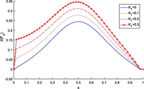
Figure 1 shows the effect of variable thermal conductivity parameter K₁ on tissue temperature distribution. It is noted that as the value of K₁ increases, the temperature increases and the temperature attains maxima at the heating position $x^{*}=0.5$. Thus, to achieve more accuracy in clinical treatments variable thermal conductivity plays an important role.

Figure 1. Dimensionless tissue temperature response along dimensionless depth with different variable conductivity parameters K₁.

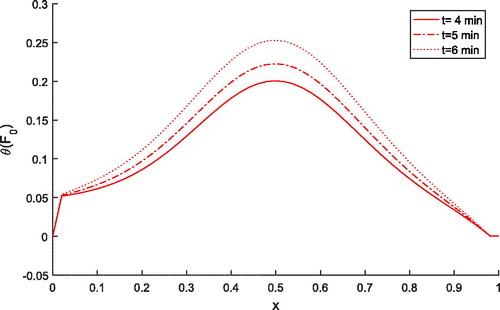
Figure 2 shows the effect of time on tissue temperature along the space coordinate when $K_1=0.1$. It is evident that temperature increases as the time increases from four minutes to six minutes during thermal ablation. Thus, it is ned that time duration affects the treatment process.

Figure 2. Dimensionless tissue temperature response along dimensionless depth with different values of time for $K_1=0.1$.

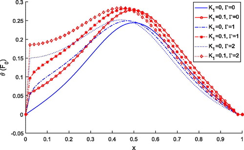
Figure 3 shows the effect of a generalized coordinate system on the treatment of tumour during thermal ablation for $K_1=0$ and $K_1=0.1$. It is noted that for all three coordinate systems, tissue temperature remains unaffected at the heating position $x^{*}=0.5$ for both the cases, but for $x>x^{*}$ and $x<x^{*}$, it affects the tissue temperature.

Figure 3. Dimensionless tissue temperature response along dimensionless depth for generalized coordinate systems.

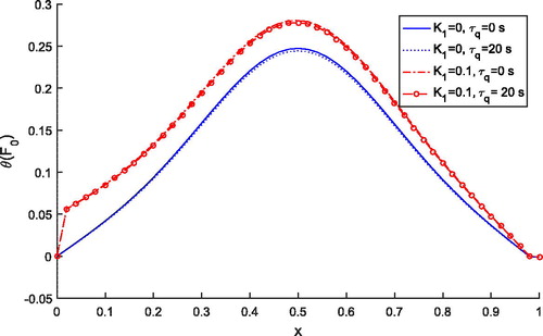
Figure 4 shows the comparison of temperature distribution for Pennes (${\tau }_q=0$) and thermal wave model $({\tau }_q=20\mathrm{s})$. It is observed that temperature profile for the thermal wave model is less than the temperature profile predicted by the Pennes’ model for both the cases of $K_1=0$ and $K_1=0.1$. But, independently, both models predict higher temperature with the variable thermal conductivity parameter. Thus, lagging time is affecting the temperature distribution during the treatment.

Figure 4. Dimensionless tissue temperature profile for different value of relaxation time.

Figure 5 shows the effects of external heat source on temperature distribution for $K_1=0$ and $K_1=0.1$. It is clear that as the value of K₁ and $q_{r0}$ increases, temperature also increases. Thus, the consideration of external heat source is important during the treatment. Figure 7 depicts the absolute error of the solutions obtained by finite element Legendre wavelet Galerkin method (FELWGM) and analytical method. Temperature (T) for time (t) 0 to 500 s is evaluated by both the methods and results are given in Table 2.

Figure 5. Dimensionless tissue temperature profile for different values of external heat source coefficient.

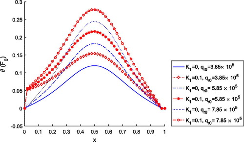
Figure 6. Plot of comparison in FELWGM solution and Exact solution.

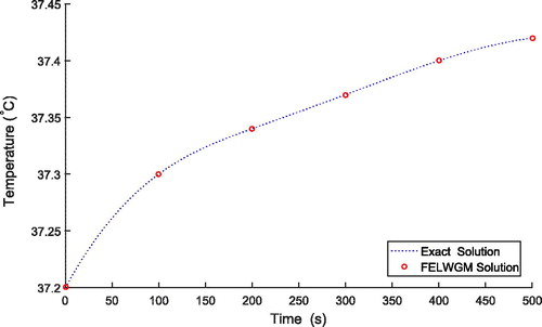
Figure 7. Absolute error.

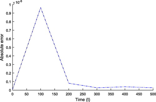
Table 2. The absolute error between the solutions obtained by FELWGM and analytical method.

Time	FELWGM	Exact solution	Absolute error
0	37.219842251500538	37.219842341320123	0.0090 $\times 1.0e-05$
100	37.319192808829554	37.319183170819544	0.9638 $\times 1.0e-05$
200	37.359167331208197	37.359166530128289	0.0801 $\times 1.0e-05$
300	37.369163646412476	37.369163921664174	0.0275 $\times 1.0e-05$
400	37.398959168730516	37.398959558330201	0.0390 $\times 1.0e-05$
500	37.409153152968211	37.409153429124091	0.0276 $\times 1.0e-05$

Therefore, we can say that the consideration of variable thermal conductivity in bioheat transfer model is very beneficial for the clinical therapeutic application in the treatment of cancerous cells.

5. Conclusions

The problem of modelling the variable thermal conductivity of thermal wave bioheat transfer model in a generalized coordinate system due to external heat source during thermal ablation has been investigated. Kirchhoff’s transformation is used to formulate the governing bioheat transfer equation. The numerical solution of the problem is achieved by using a finite difference scheme and Legendre wavelet Galerkin approach. FELWGM converts the problem into a system of algebraic equation, so it reduces the computational complexity and avoids large storage requirements, as in the case of conventional discretize schemes. The results obtained from the FELWGM are compared with the analytical results and give good accuracy in the absence of external heat source. The significant effect of variable thermal conductivity parameters, variability of time, lagging times, and external heat source is observed on tissue temperature distribution. Therefore, the temperature dependent changes need to be considered to enhance the accuracy of predicting and monitoring pre-clinical and clinical treatments and consideration of this model is useful in image-guided thermal treatments (e.g. hyperthermia and thermal ablation) and other biomedical treatments. It will give new direction in clinical therapeutic application.

Nomenclature
Γ	=	the number of classify coordinate
κ	=	tissue thermal diffusivity, m2s−1
ωb	=	blood perfusion rate, s−1
ρ	=	tissue density, kgm−3
ρb	=	blood mass density, kgm−3
τq	=	heat flux relaxation time, s
Θ	=	dimensionless tissue temperature, in Equation (28)(28) $$F_{0q}\frac{{\partial }^2\Theta }{\partial F_0^2}+\left(1+F_{0q}{P}_f^2-F_{0q}{P}_{m0}d\right)\frac{\partial \Theta }{\partial F_0}-\left(P_{m0}d-P_f^2\right)\Theta =\frac{{\partial }^2\Theta }{\partial x^2}+\frac{\Gamma }{x}\frac{\partial \Theta }{\partial x}+P_f^2{\vartheta }_a+P_{m0}+P_{r0}{\mathrm{e}}^{-a^2{\left(x-x^{*}\right)}^2},$$(28)
θ	=	dimensionless tissue temperature
${\vartheta }_a$	=	dimensionless arterial blood temperature
${\vartheta }_w$	=	dimensionless wall temperature at boundary
a0	=	scattering parameter, m−1
c	=	specific heat of tissue, jkg−1
cb	=	specific heat of blood, jkg−1k−1
$F_{0q}$	=	dimensionless heat flux relaxation time
F0	=	dimensionless time
k	=	variable thermal conductivity of tissue, Wm−1K−1
k0	=	constant thermal conductivity of tissue, Wm−1K−1
K1	=	dimensionless variable thermal conductivity parameter
k1	=	variable thermal conductivity parameter, °C−1
L	=	tissue slab length, m
l	=	Bromwich contour integration line
P	=	transmitted power, W
Pf	=	dimensionless blood perfusion coefficient
$P_{m0}$	=	dimensionless metabolic heat source coefficient
$P_{r0}$	=	dimensionless external heat source coefficient
qb	=	heat source due to blood perfusion, Wm−3
qm	=	heat source due to metabolic heat generation, Wm−3
qs	=	external heat source, Wm−3
$q_{m0}$	=	constant metabolic heat source
$q_{r0}$	=	reference external heat source, Wm−3
r	=	space coordinate, m
r0	=	location of tumor, m
S	=	antenna power, m−1
s	=	Laplace domain parameter
T	=	tissue temperature, °C
t	=	time, s
T0	=	initial temperature of body, °C
Ta	=	arterial blood temperature, °C
Tw	=	wall temperature at the boundary, °C
x	=	dimensionless space coordinate
$x^{*}$	=	dimensionless location of tumor where heat is applied

Acknowledgement

The third author is thankful to the Council of Scientific and Industrial Research (CSIR), India, for providing fellowship under the SRF(21/06/2015/(i)EU-V) scheme.

Disclosure statement

The authors have no conflict of interest.

References

- Akbar, N. S., Raza, M., & Ellahi, R. (2016a). Anti-bacterial application for new thermal conductivity model in arteries with CNT suspended nanofluid. Journal of Mechanics in Medicine and Biology, 16(5), 1650063. doi: 10.1142/S0219519416500639
- Akbar, N. S., Raza, M., & Ellahi, R. (2016b). Endoscopic effects with entropy generation analysis in peristalsis for the thermal conductivity of H2O+Cu nanofluid. Journal of Applied Mathematics and Mechanics, 9(4), 1721–1730.
- Arpaci, V. S. (1996). Conduction heat transfer. Reading, MA: Addison-Wesley Publishing Co.
- Bhattacharya, A., & Mahajan, R. L. (2003). Temperature dependence of thermal conductivity of biological tissues. Physiological Measurement, 24(3), 769–783. doi: 10.1088/0967-3334/24/3/312
- Bhatti, M. M., Zeeshan, A., & Ellahi, R. (2017). Electromagnetohydrodynamic (EMHD) peristaltic flow of solid particles in a third-grade fluid with heat transfer. Mechanics & Industry, 18(3), 314. doi: 10.1051/meca/2016061
- Bhatti, M. M., Zeeshan, A., Ellahi, R., & Shit, G. C. (2018). Mathematical modeling of heat and mass transfer effects on MHD peristaltic propulsion of two-phase flow through a Darcy–Brinkman–Forchheimer porous medium. Advanced Powder Technology, 29(5), 1189–1197. doi: 10.1016/j.apt.2018.02.010
- Bhatti, M. M., Zeeshan, A., Tripathi, D., & Ellahi, R. (2018). Thermally developed peristaltic propulsion of magnetic solid particles in biorheological fluids. Indian Journal of Physics, 92(4), 423–430. doi: 10.1007/s12648-017-1132-x
- Cattaneo, C. (1958). A form of heat conduction equation which eliminates the paradox of instantaneous propagation. Compte Rendus, 247, 431–433.
- Ellahi, R., Alamri, Sultan, Z., Basit, A., & Majeed, A. (2018). Effects of MHD and slip on heat transfer boundary layer flow over a moving plate based on specific entropy generation. Journal of Taibah University for Science, 12(4), 476–482. doi: 10.1080/16583655.2018.1483795
- Ellahi, R., Zeeshan, A., Shehzad, N., & Alamri, S. Z. (2018). Structural impact of kerosene-Al2O3 nanoliquid on MHD Poiseuille flow with variable thermal conductivity: Application of cooling process. Journal of Molecular Liquids, 264, 607–615. doi: 10.1016/j.molliq.2018.05.103
- Guntur, S. R., & Choi, M. J. (2015). Influence of temperature-dependent thermal parameters on temperature elevation of tissue exposed to high-intensity focused ultrasound: Numerical simulation. Ultrasound in Medicine and Biology, 41(3), 806–813. doi: 10.1016/j.ultrasmedbio.2014.10.008
- Guntur, S. R., Lee, K. I., Paeng, D. G., Coleman, A. J., & Choi, M. J. (2013). Temperature-dependent thermal properties of ex vivo liver undergoing thermal ablation. Ultrasound in Medicine and Biology, 39, 1–14.
- Gupta, P. K., Singh, J., & Rai, K. N. (2010). Numerical simulation for heat transfer in tissues during thermal therapy. Journal of Thermal Biology, 35(6), 295–301. doi: 10.1016/j.jtherbio.2010.06.007
- Hassan, M., Marin, M., Ellahi, R., & Alamri, S. Z. (2018). Exploration of convective heat transfer and flow characteristics synthesis by Cu–Ag water hybrid-nanofluids. Heat Transfer Research, 49(18), 1837–1848. doi: 10.1615/HeatTransRes.2018025569
- Hetnarski, R. B. (1986). Thermal Stresses, Vol. I. North-Holland, Amsterdam: Taylor and Francis Group.
- Ijaz, N., Zeeshan, A., Bhatti, M. M., & Ellahi, R. (2018). Analytical study on liquid-solid particles interaction in the presence of heat and mass transfer through a wavy channel. Journal of Molecular Liquids, 250, 80–87. doi: 10.1016/j.molliq.2017.11.123
- Kashcooli, M., Salimpour, M. R., & Shirani, E. (2017). Heat transfer analysis of skin during thermal therapy using thermal wave equation. Journal of Thermal Biology, 64, 7–18. doi: 10.1016/j.jtherbio.2016.12.007
- Kumar, D., & Rai, K. N. (2017). Numerical simulation of time fractional dual-phase-lag model of heat transfer within skin tissue during thermal therapy. Journal of Thermal Biology, 67, 49–58. doi: 10.1016/j.jtherbio.2017.05.001
- Kumar, D., Kumar, P., & Rai, K. N. (2015a). Numerical Study on non-Fourier bioheat transfer during thermal ablation. Procedia Engineering, 127, 1300–1307. doi: 10.1016/j.proeng.2015.11.487
- Kumar, D., Singh, S., Sharma, N., & Rai, K. N. (2018). Verified non-linear DPL model with experimental data for analyzing heat transfer in tissue during thermal therapy. International Journal of Thermal Sciences, 133, 320–329. doi: 10.1016/j.ijthermalsci.2018.07.031
- Kumar, P., Kumar, D., & Rai, K. N. (2015b). A numerical study on dual-phase-lag model of bio-heat transfer during hyperthermia treatment. Journal of Thermal Biology, 49–50, 98–105. doi: 10.1016/j.jtherbio.2015.02.008
- Kumar, P., Kumar, D., & Rai, K. N. (2016). Non-linear dual-phase-lag model for analyzing heat transfer phenomena in living tissues during thermal ablation. Journal of Thermal Biology, 20, 204–212. doi: 10.1016/j.jtherbio.2016.07.017
- Kumar, S., Damor, R. S., & Shukla, A. K. (2018). Numerical study on thermal therapy of triple layer skin tissue using fractional bioheat model. International Journal of Biomathematics, 11(04), 1850052. doi: 10.1142/S1793524518500523
- Pennes, H. H. (1948). Analysis of tissue and arterial blood temperature in the resting forearm. Journal of Applied Physiology, 1(2), 93–122. doi: 10.1152/jappl.1948.1.2.93
- Razzaghi, M., & Yousefi, S. (2001). The Legendre wavelets operational matrix of integration. International Journal of Systems Science, 32(4), 495–502. doi: 10.1080/002077201300080910
- Rossmann, C., & Haemmerich, D. (2014). Review of temperature dependence of thermal properties, dielectric properties, and perfusion of biological tissues at hyperthermic and ablation temperatures. Critical Reviews in Biomedical Engineering, 42, 467–492. doi: 10.1615/CritRevBiomedEng.2015012486
- Tan, Q., Zou, X., Dong, H., Ding, Y., & Zhao, X. (2018). Influence of blood vessels on temperature during high-intensity focused ultrasound hyperthermia based on the thermal wave model of bioheat transfer. Advances in Condensed Matter Physics, 2018, 5018460. doi: 10.1155/2018/5018460
- Trujillo, M., & Berjano, E. (2013). Review of the mathematical functions used to model the temperature dependence of electrical and thermal conductivities of biological tissues in radiofrequency ablation. International Journal of Hyperthermia, 29(6), 590–597. doi: 10.3109/02656736.2013.807438
- Valvano, J. W., Cochran, J. R., & Diller, K. R. (1985). Thermal conductivity and diffusivity of biomaterials measured with self-heated thermistors. International Journal of Thermophysics, 6(3), 301–311. doi: 10.1007/BF00522151
- Vernotte, P. (1958). Les paradoxes de la theorie continue de l’equation de la chaleur. Compte Rendus, 246, 3154–3155.
- Watanabe, H., Kobayashi, Y., Hashiszume, M., & Fujie, M. G. (2009). Modeling the temperature dependence of thermophysical properties: Study on the effect of temperature dependence for RFA, 31st Annual International Conference of the IEEE EMBS Minneapolis, Minnesota, USA, September 2–6.
- Yadav, S., Kumar, D., & Rai, K. N. (2014). Finite element Legendre wavelet Galerkin approach to inward solidification in simple body under most generalized boundary condition. Zeitschrift für Naturforschung, 69a, 501–510.