Permutation rules and genetic algorithm to solve the traveling salesman problem

Abstract

In this paper, a new approach including permutation rules and a genetic algorithm is proposed to solve the symmetric travelling salesman problem. This problem is known to be NP-Hard. In order to increase the efficiency of the genetic algorithm, the initial population of feasible solutions is carefully generated. In addition to that, dynamic crossover and mutation rates were developed. The proposed method was successfully tested using large numbers of different-sized benchmarks. The computational results proved that the proposed solution approach outperforms many existing methods. In addition, for many problem instances the proposed algorithm is able to generate solutions with same value as the best known solutions.

Keywords:

• TSP
• genetic algorithms
• permutation rules
• dynamic rates

1. Introduction and background

The travelling salesman problem (TSP) is a popular and challenging optimization problem and belongs to the class of NP-complete problems. In this problem, the salesman aims to visit all the cities and return to the start city with the constraint that each city can be visited only once. The classical objective is to minimize the total travelled distance. The TSPs are real world problems related to transportation, logistics, etc. In transportation, the school buses routes are established to find a cheapest link through every stop. Another real life application can be found in transportation in logistics where the aim is to find the cheapest route to deliver goods to customers. Thus, proposing solutions for them is of great interest (Osaba, Yang, Diaz, Garcia, & Carballedo, 2016). Most of the real world TSPs are very complex. Therefore, finding an optimal solution within an accepted time is a big challenge. In line with this, any related TSP problem is hard to solve using exact procedures (Lawler, Lenstra, Kan, & Shmoys, 1985).

Various heuristics and approximation algorithms have been developed in the last few decades. In addition, many local optimization techniques such as simulated annealing, tabu search, neural networks and genetic algorithms (see Aarts, Korst, & van Laarhoven, 1988; Fiechter, 1994; Gendreau, Laporte, & Semet, 1998; Grefenstette, Gopal, Rosmaita, & VanGucht, 1985; Knox, 1994; Larranaga, Kuijpers, Murga, Inza, & Dizdarevic, 1999; Leung, Jin, & Xu, 2004; Malek, Guruswamy, Pandya, & Owens, 1989) were developed. Hybrid algorithms were also proposed to solve efficiently the TSP. In Chen and Chien (2011), the authors proposed a hybridization of the genetic algorithm, the simulated annealing and the ant colony system with particle swarm optimization techniques. The experimental results showed that the proposed solution approach gives better average solution and percentage deviation of the average solution than existing methods. The authors in Dong, Guo, and Tickle (2012) proposed a new hybrid algorithm, cooperative genetic ant system (CGAS). This new approach combines cooperatively both Genetic Algorithm (GA) and Ant Colony Optimization (ACO) with the aim to improve the performance of ACO. The experimental results of CGAS are better than those of GA and ACO algorithms in terms of quality of average optimal solutions, particularly for small TS problems. Masutti and De Castro (2009) investigated a TSP problem. They proposed a solution approach by modifying the RABNET-TSP (an immune-inspired self-organizing neural network). The algorithm is then compared with other neural network-based methods proposed in the literature. The overall results were promising and better even though the algorithm requires longer processing time for convergence in many cases. The symmetric and asymmetric TSPs were studied in Osaba et al. (2016) and Osaba, Javier, Sadollah, Bilbao, and Camacho (2018). To solve these problems, the authors proposed an improvement of the classic bat algorithm as well as a discrete water cycle algorithm. Another type of TSP is called Family Travelling Salesman Problem (FTSP) and has attracted many researchers. In this problem, instead of knowing exactly the cities to be visited, we only know how many cities to visit in a subset of cities, which is called a family. For example, we can cite Bernardino and Paias (2018). In their paper, the authors proposed exact and heuristic procedures to solve the FTSP. In addition, compact and non-compact models were theoretically and practically compared. In the classical TSP, the distance from the city is fixed and known in advance. This assumption may not be always true where this distance may be subject to changes. Therefore, this problem is referred to as dynamic TSP as studied by Mavrovouniotis, Muller, and Yang (2017).

Furthermore, meta-heuristics inspired by biological structures and processes were developed to solve the TSP. Some of these meta-heuristics are the firefly algorithm (Jati, Manurung, & Suyanto, 2013; Li, Ma, Zhang, Zhou, & Liu, 2015), the Cuckoo Search (Ouaarab, Ahiod, & Yang, 2014) and the Imperialist Competitive Algorithm (Ardalan, Karimi, Poursabzi, & Naderi, 2015; Yousefikhoshbakht & Sedighpour, 2013).

Real world TSPs are of large sizes. This fact motivated (Taillard & Helsgaun, 2019) to propose a metaheuristic to optimize locally sub-parts of a solution to a given problem. This heuristic can be used as part of many neighbourhood search methods. The authors showed that it finds efficiently high quality solutions.

The main contribution of this paper is the development of a Genetic Algorithm that solves the symmetric TSP. Usually, the initial population is randomly generated. However, in this work we proposed permutation rules to start with relatively good solutions. In addition, to help the genetic algorithm converge toward optimal or near optimal solutions, we proposed a dynamic crossover rate that depends on the population being considered.

This paper is organized as follows. The studied TSP is defined and formulated in Section 2. Section 3 describes the proposed method used to solve the TSP. Section 4 presents the testing and simulation results in addition to discussion and analysis of the obtained results. Section 5 concludes the paper and proposes some recommendations to improve the current solution approach as well as including more constraints to deal with more realistic TSPs.

2. Problem definition and formulation

The Travelling Salesman Problem (TSP) is one of the famous and well-studied problems in operations research fields. The problem is considered to be NP-hard and is of great interest (Lawler et al., 1985). Hence, it has attracted many researchers.

Different versions of the travelling salesman problem exist based on the definition of the distances between the cities. The problem is said to be symmetric if for every pair of cities (a, b), the distance from city a to city b is the same as the distance from city b to city a. The problem is said to be asymmetric if this property does not hold. In addition, the problem is said to be Euclidean if the distance between two cities is the Euclidean distance. In this study we consider a symmetric and Euclidean TSP. Many real world applications of the TSP problem exist such as computer wiring, order-picking and overhauling gas turbine engines (Matai, Mittal, & Singh, 2010).

The TSP can be defined on a complete undirected graph $G=(V,E),$ where $V=\{1,2,\dots ,n\}$ is the set of n vertices and $E=\{(i,j);i,j\in \mathit{Vandi}\ne j\}$ the set of edges (connections between cities). Figure 1 shows the graphical representation of the TSP described in Table 1. A cost c_ij (can be distance, time, etc.) is assigned to each edge (i, j), where all the costs satisfy the constraint $c_{\mathit{ij}}\le c_{\mathit{ik}}+c_{\mathit{kj}}$ for all $i,j,k\in V.$ In the current study, the vertices are assumed to be points $P_i=(X_i,Y_i)$ in the plane and $c_{\mathit{ij}}=\sqrt{{(X_i-X_j)}^2+{(Y_i-Y_j)}^2}$ the Euclidean distance between P_i and P_j. The distances c_ij can be represented by a symmetric square matrix C as shown in Table 1 describing a symmetric salesman problem of five cities.

Figure 1. Graphical representation of the TSP shown in Table 1.

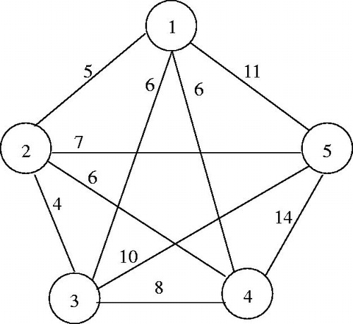
Table 1. Traveling salesman problem of five cities.

Cities	1	2	3	4	5
1	0	5	6	6	11
2	5	0	4	6	7
3	6	4	0	8	10
4	6	6	8	0	14
5	11	7	10	14	0

A feasible solution to the TSP is a tour T formed by a sequence of n selected edges pairwise distinct allowing to visit the n cities without redundancy except the start city which appears at the beginning and the end of the tour. In addition to the graphical representation, the TSP can be formulated as an Integer programming problem as shown in the following subsections.

2.1. Decision variables

Equation (1)(1) $$x_{\mathit{ij}}\in \{0,1\}\forall (i,j)\in E$$(1) defines a binary variable x_ij associated with each edge (i, j) in the graph G. The values 1 and 0 of x_ij indicate respectively the inclusion or exclusion of every edge (i, j) in the optimal tour. (1) $$x_{\mathit{ij}}\in \{0,1\}\forall (i,j)\in E$$(1)

2.2. Objective function

The objective expressed in Equation (2)(2) $$\mathit{Min}\sum _{i,j\in V;i<j}{c}_{\mathit{ij}}{x}_{\mathit{ij}}$$(2) is to find the shortest tour. (2) $$\mathit{Min}\sum _{i,j\in V;i<j}{c}_{\mathit{ij}}{x}_{\mathit{ij}}$$(2)

2.3. Constraints

The constraints to be considered are formulated in this section. Any feasible tour, including the optimal tour, must contain exactly n edges asl expressed in Equation (3)(3) $$\sum _{i,j\in V}{x}_{\mathit{ij}}=n$$(3) . (3) $$\sum _{i,j\in V}{x}_{\mathit{ij}}=n$$(3)

Equation (4)(4) $$\sum _{i<k}{x}_{\mathit{ik}}+\sum _{k<j}{x}_{\mathit{kj}}=2$$(4) states that only two edges must be selected for each vertex. This constraint allows to produce tours where every city is visited only once and the salesman returns back to the start city. (4) $$\sum _{i<k}{x}_{\mathit{ik}}+\sum _{k<j}{x}_{\mathit{kj}}=2$$(4)

Finally, Equation (5)(5) $$\sum _{i<j}{x}_{\mathit{ij}}\le \left|T\right|-1(T\subset V,\hspace{1em}2\le |T|\le n-2)$$(5) prohibits the formation of sub tours containing a number of vertices smaller than n. This constraint guarantees the visit of all cities. (5) $$\sum _{i<j}{x}_{\mathit{ij}}\le \left|T\right|-1(T\subset V,\hspace{1em}2\le |T|\le n-2)$$(5)

3. Solution approach

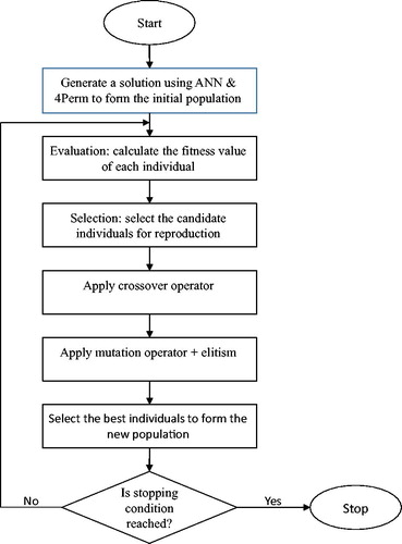
In this section, we describe in detail the proposed genetic algorithm to solve the travelling salesman problem. The motivation behind using Genetic Algorithms (GAs) is that they are simple and powerful optimization techniques to solve NP-hard problems. GAs start with a population of feasible solutions to an optimization problem and apply iteratively different operators to generate better solutions. These operators, based on random processes, allow GAs to explore the search space in different directions. GAs evaluate each individual of the population using a fitness function. Most fitted individuals are selected for reproduction with the aim of getting better feasible solutions. The reproduction process includes crossover and mutation operators. The evaluation, selection and reproduction are repeated until some stopping conditions are reached. The different components used to develop the genetic algorithm are detailed in the next subsections. The process of the PGAs is described in Figure 2.

Figure 2. Genetic algorithm flowchart diagram.

3.1. Encoding

The genotype of the individuals (chromosomes) is represented by a sequence of n integers with no repeated values. This kind of path representation is simple to implement and provides chromosomes directly interpreted as TSP’s solutions (tours). A chromosome Cr can be formulated as $\mathit{Cr}=(g_1,g_2,\dots ,g_n)$ where $g_i\in V,1\le i\le n$ represents a gene (node) in the chromosome. An example of chromosome for the TSP instance shown in Table 1 is $1,3,4,5,2,6.$ The resulting tour $1,3,4,5,2,6,1$ is obtained from the chromosome by appending the initial city at the end.

3.2. Initial population

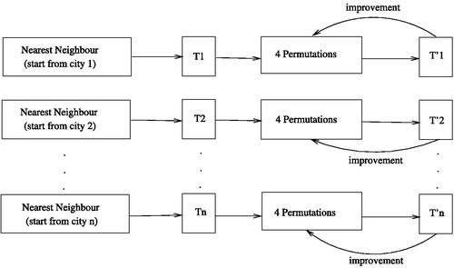
Generating the initial population is a very important step in the GA. Usually, the initial population is randomly generated. In this paper, the initial population is carefully created to guarantee better and faster convergence toward the optimal or near optimal solutions. The initial population for the developed genetic algorithm was generated using two proposed heuristics. The first heuristic, named ANN is a generalization of the well known Nearest Neighbour approach. The second heuristic, namely 4Perm, aims to improve the solutions obtained by ANN by applying some permutation rules. These heuristics will be detailed in the next paragraphs.

3.2.1. All nearest neighbors (ANN)

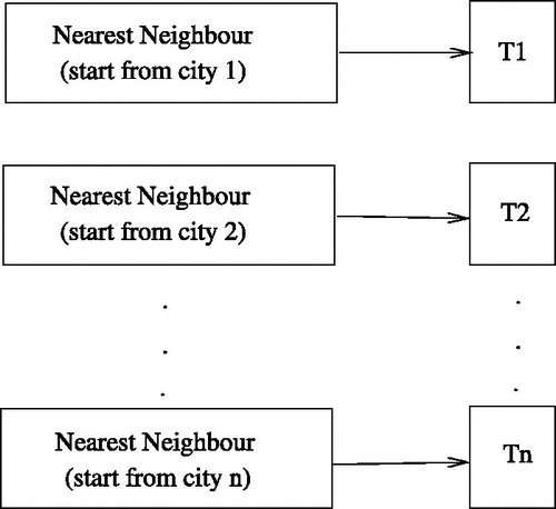
ANNis a generalization of the classical Nearest Neighbor heuristic (NN) that consists of constructing a solution to the TSP starting always from city 1 (initial city). In every step, the salesman has to visit the non-visited city next nearest to his current location. We generalized this rule to generate n tours T_i, $(1\le i\le n),$ where each tour T_i starts from city i. The reason behind this is simply because all the generated tours via some rotations will all start from the initial city 1. But, the intermediate cities will have different orders of visits. ANN is described in Figure 3.

Figure 3. Diagram describing ANN.

Computational complexity

First, we study the computational complexity of the nearest neighbour heuristic NN which starts from the city 1. Step 1 consists of selecting the nearest city to city 1. This step requires the comparison of $(n-1)$ edges $(1,2),(1,3),\dots ,(1,n)$ to select the edge with minimum cost. In step 2, we compare $(n-2)$ edges and so on until there is only one edge. Therefore, there are $(n-1)+(n-2)+\dots +1=\frac{n(n-1)}{2}$ comparisons. Since ANN generates n different tours, each starts from a distinct first node, and the computational complexity of ANN is of the order of $O(n^3).$

3.2.2. Four permutation rules-based heuristic (4Perm)

The idea of the second heuristic is to check whether or not successive local and slight changes of a tour can lead to a better one. Since graphically a tour can be represented as a Hamiltonian cycle, replacing two carefully-selected edges (i, j) and (k, l) from the tour having no common city with two other edges that are not in the tour, can lead to a new and more feasible tour. Following are four proposed rules to perform the edge permutations in a feasible tour T with n edges. The digit 1 in the rule’s name indicates the addition of an edge $(i,j)\in E,$ which is currently not in the tour, to the tour. However, the digit 0 indicates the removal of an edge from the tour.

• Rule 1 (Perm₀₀₁₁): Delete the edge $(i,j)\in T$ having the highest cost c_ij from the tour. Then, delete the edge $(k,l)\in T$ having the second highest cost c_kl and that has no common city with the edge $(i,j).$ Finally, replace the deleted edges by their crossings $(i,l)\notin T$ and $(j,k)\notin T$

• Rule 2 (Perm₁₁₀₀): Add to the tour the edge $(i,j)\notin T$ having the lowest cost c_ij. Then, insert the edge $(k,l)\notin T$ having the second lowest cost c_kl and that has no common city with the edge $(i,j).$ Finally, delete the edges (i, k) and (l, j) from the tour.

• Rule 3 (Perm₁₀₁₀): Add to the tour the edge $(i,j)\notin T$ having the lowest cost c_ij. Then, compare the costs of the four edges $(i,i_1),(i,i_2),(j,j_1)$ and $(j,j_2)$ that belong to the tour and neighbours to the cities i and j to exclude the edge with the highest cost. Without loss of generality, suppose that the edge $(j,j_1)$ was excluded from the tour. Next, add to the tour the edge (j₁, i₂) or the edge (j₁, i₁) (the one that keeps the tour feasible); say $(j_1,i_2).$ Finally, delete the edge $(i,i_2)$ from the tour.

• Rule 4 (Perm₀₁₀₁): Delete from the tour the edge $(i,j)\in T$ having the highest cost c_ij. Then, insert an edge from the set $\{(i,k)\notin T\mathit{and}(j,k)\notin T,k\in V\}$ having the lowest cost, say for example $(i,k).$ Next, delete the edge $(k,l)\in T$ so that the insertion of the edge $(l,j)\notin T$ to T keeps T feasible.

To illustrate the above described process, the permutation rules were applied to the TSP instance shown in Figure 1. The results are detailed in Figure 4. For example, Perm₀₀₁₁ deletes the edges (1, 3) and (4, 5) and inserts the edges (1, 5) and (4, 3) into the tour. The resulting tour has a length slightly smaller than the initial one. It is clear from this figure that the four rules apply a slight perturbation to a given tour but the improvement in cost is not always guaranteed. Even an increase of the total cost of the resulting tour may occur. Figure 4 shows a cost improvement of the initial tour T₀ using the rules Perm₀₀₁₁ and Perm₀₁₀₁ and a cost increase given by the rules Perm₁₁₀₀ and Perm₁₀₁₀.

Figure 4. Illustration of the four permutation rules.

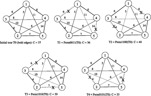
It is also obvious that the improvement of a given tour cannot be always obtained by applying a special permutation rule. Thus, applying them altogether is the best way to guarantee a high chance of cost improvement. In addition to that, applying these rules iteratively to a given tour may also lead to the best nearest tour (local optima).

The aim of 4Perm heuristic is to improve the solutions generated by ANN. The idea is to iteratively apply the four permutation rules to every solution. At every iteration, the best tour obtained is kept for the next iteration. This step generates n new tours with lower costs. This process is iteratively repeated until no more cost improvement is obtained. Figure 5 illustrates the heuristic process.

Figure 5. 4Perm process diagram.

Computational complexity

It is not evident to estimate the computational complexity of the 4Perm heuristic. The reason is that there are n loops during every one of them and a given tour is slightly modified using the four permutation rules until there is no more improvement. However, the experimental study showed that the considered loops stops quickly even for large size instances and the improvement of every tour is very small as shown in Table 2. We can confirm according to the experimental study that the computational complexity of the 4Perm method is polynomial.

Table 2. Testing results of ANN and 4Perm heuristics.

Pb. No.	n	Benchmark	CANN	$C_{4P\mathit{erm}}$	$C^{*}$	$p{e}_{4P\mathit{erm}}$
1	51	eil51	482	482	426	13.1
2	52	Berlin52	8181	8181	7542	8.5
3	70	St70	796	796	675	3.1
4	76	eil76	608	591	538	9.9
5	99	rat99	1471	1460	1211	20.6
6	100	kroB100	25,884	25,884	22,141	16.9
7	100	kroA100	24,698	24,524	21,282	15.2
8	100	rd100	9423	9415	7910	19
9	101	eil101	746	746	629	18.6
10	105	in105	16,935	16,703	14,379	16.2
11	130	ch130	7129	7090	6110	16.0
12	150	ch150	7113	7113	6528	9.0
13	198	d198	17,620	17,620	15,780	11.7
14	200	kroA200	34,543	34,471	29,368	17.4

3.3. Evaluation

The evaluation function is used to assign to each chromosome in the population a fitness value. For the TSP problem, the fitness value is the inverse of the resulting tour’s length. Therefore, the higher the fitness, the better the chromosome. The fitness function f of a chromosome $\mathit{Cr}=(g_1,g_2,\dots ,g_n)$ is given by Equation (6)(6) $$f\left(\mathit{Cr}\right)=\frac{1}{c_{g_n{g}_1}+{\sum }_{i=1}^{n-1}{c}_{g_i{g}_{i+1}}}$$(6) . (6) $$f\left(\mathit{Cr}\right)=\frac{1}{c_{g_n{g}_1}+{\sum }_{i=1}^{n-1}{c}_{g_i{g}_{i+1}}}$$(6)

3.4. Selection

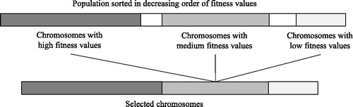
The selection is inspired from the natural phenomena that promote fitter individuals for reproduction. Meanwhile, some individuals with medium or even low fitness can be useful to introduce their good characteristics in the next generations. We followed this principle for the selection of chromosome candidates. The population is sorted in a decreasing order of the chromosomes’ fitness values. Then, most of the current fittest chromosomes, some with medium fitness, and a few weak individuals are selected. The selection of the chromosomes for the reproduction phase proceeds as follows. Fifty per cent% of the population is selected representing the fittest chromosomes. Then 20% of chromosomes with medium fitness values and the last 10% of the chromosomes are selected. This process is illustrated in Figure 6.

Figure 6. Genetic algorithm selection operator.

3.5. Crossover

The crossover operator is the most important component of the GA. The process of crossover consists of combining two individuals to create new ones. These newly created chromosomes are then copied into the new population. In this study, many crossover operators were empirically tested with the aim to choose the most suitable one(s). Two different crossover operators were used, namely Ordered Crossover (OX) proposed by Goldberg (1989) and Sequential Constructive Crossover (SCX) proposed by Zakir (2010).

3.6. Mutation

The mutation is used so that the genetic algorithm does not get stacked in a local optimum. It is used to maintain the genetic diversity in the population. This operator modifies the genes of a chromosome selected with a mutation probability p_m. Different mutation operators were empirically tested. Four different mutation operators proposed by Sivanandam and Deepa (2007), namely Interchanging Mutation (IM), Reversing Mutation (RM), Swap Mutation (SWM) and Reverse Sequence Mutation (RSM) have been selected in this study.

3.7. Insertion method

The insertion method consists of copying the best chromosome from the old population to the new generation (Chakraborty & Chaudhuri, 2003). The solutions resulting from the crossover and mutation stages are also added to the new population so that the population size remains fixed from one generation to another. This method of forming the new population guarantees the convergence of the GA to a global optimal solution.

3.8. New dynamic crossover and mutation rates

Since the mutation and particularly the crossover rates have an impact on the efficiency of the solutions generated by the genetic algorithm, the aim of this method is that the crossover and mutation rates are no more fixed but vary from one generation to another. The aforementioned rates depend on the maximum fitness f_max and average fitness f_avg among the individuals in the population as well as the best known fitness f_bkn. This idea was inspired from Li (2010). The new dynamic crossover and mutation rates are illustrated in Equations (7)(7) $$p_c=k_1\times \frac{(f_{\mathit{max}}-f_{\mathit{avg}})}{(f_{\mathit{bkn}}-f_{\mathit{max}})}$$(7) and (8)(8) $$p_m=k_2\times \frac{(f_{\mathit{max}}-f_{\mathit{avg}})}{(f_{\mathit{bkn}}-f_{\mathit{max}})}$$(8) , respectively. (7) $$p_c=k_1\times \frac{(f_{\mathit{max}}-f_{\mathit{avg}})}{(f_{\mathit{bkn}}-f_{\mathit{max}})}$$(7) (8) $$p_m=k_2\times \frac{(f_{\mathit{max}}-f_{\mathit{avg}})}{(f_{\mathit{bkn}}-f_{\mathit{max}})}$$(8) where k₁ and k₂ are parameters varying in $[0,1]$ to promote some chromosomes to be selected for crossover mutation depending on their fitness values. The chromosomes with high fitness value will have more chance to be selected and vice versa. This process will probably help in producing fitter chromosomes in future generations.

3.9. Genetic algorithm parameter tuning

The genetic algorithm parameters values were empirically tuned. The population size is 100. The genetic algorithm was run 50 independent times. In each run, the cycle of the genetic algorithm going from evaluation of the current population until applying the mutation is repeated 100 times. The best solution over each run is saved. Finally, the best solution over all the 50 runs is returned. Applying dynamic crossover and mutation operators with variable probability values guarantees the convergence of the GA toward good solutions. The experimental results confirmed this as the obtained results are in general very promising. Moreover, multiple tests were conducted to adjust the values of the different genetic algorithm parameters. It was noticed that the best values for the parameters k₁ and k₂ are 0.6 and 0.1, respectively.

4. Experimental results

The ANN and 4Perm heuristics were coded in Python (Version 3.5.x), whereas the proposed genetic algorithm was implemented using Java language on a MacBook Pro 2.5 GHz Intel core i5.

In order to validate the performance of the developed methods, many benchmarks with different sizes have been used from the TSPLIB website (Reinelt, 1997). We first tested the heuristics ANN and 4Perm. The computational results are summarized in Table 2 where C_ANN and $C_{4P\mathit{erm}}$ represent the lengths of the tours generated by ANN and 4Perm, respectively, and $C^{*}$ is the best-known tour length. We define the percentage error pe_H given by Equation (9)(9) $$p{e}_H=\frac{C_H-C^{*}}{C^{*}}\times 100$$(9) as a measure of how far are the best solutions generated by a heuristic H to the best known solution. The results show clearly better performance of 4Perm compared to ANN. The last column of Table 2 shows that the percentage error of 4Perm compared to the best known solutions varies from 8.5 to 21.6. This can be explained by the fact that ANN and 4Perm do not have enough ability to avoid local minima. Therefore, the genetic algorithm is used to improve the quality of the solutions generated by ANN and 4Perm. (9) $$p{e}_H=\frac{C_H-C^{*}}{C^{*}}\times 100$$(9)

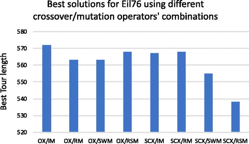
It was also noted from the computational results that SCX crossover along with Reverse Sequence Mutation (RSM) outperform all other crossover/mutation combinations for almost all the tested problems. Figure 7 shows the experimental results obtained for Eil76 dataset using different crossover/mutation operators’ combinations. From that figure we can see that SCX/RSM is the best crossover/mutation combination.

Figure 7. Best solutions for Eil76 using different crossover/mutation operators’ combinations.

Table 3 shows a comparison of the experimental results of the best solution C_GA (cost provided by the proposed genetic algorithm) with the best known solution $C^{*}.$ Different combinations of crossover and mutation operators were used. When examining Table 3, it can be seen that the proposed method solves optimally four instances and provides solutions with costs too close to the optimal for all other instances. Table 4 shows that the proposed method was able to generate the same or better solutions than most of the selected methods used for comparison.

Table 3. Testing results of the proposed GA.

Pb. No.	n	Benchmark	CGA	$C^{*}$	peGA
1	51	eil51	427	426	0.23
2	52	Berlin52	$7542$	7542	0
3	70	St70	$675$	675	0
4	76	eil76	$538$	538	0
5	99	rat99	1218	1211	0.5
6	100	kroB100	22,407	22,141	1.2
7	100	kroA100	21,292	21,282	0.04
8	100	rd100	8020	7910	1.39
9	101	eil101	630	629	0.15
10	105	in105	14,434	14,379	0.38
11	130	ch130	6283	6110	2.8
12	150	ch150	6580	6528	0.8
13	198	d198	15,884	15,780	0.6
14	200	kroA200	$29368$	29,368	0

Table 4. Comparison of PGA performance with other methods in the literature.

	Problem
	$C^{*}$
Method (reference)	Eil51	Berlin52	Rat99	Eil76	St70	KroA100	Lin105	KroA200	Ch150	Eil101
	426	7542	1211	538	675	2,1282	14,379	29,368	6528	629
ACOMAC (Tsai, Tsai, & Tseng, 2004)	430.68	–	–	555.70	–	21,457	–	–	–	–
ACOMAC + NN (Tsai et al., 2004)	430.04	–	–	553.94	–	21,433.33	–	–	–	–
RABNET-TSP (Pasti & De Castro, 2006)	427	7542	–	541	678.84	21,333	14,379	29,600	6602	638
Modified RABNET-TSP (Masutti & De Castro, 2009)	429	7716	–	542	–	21,369	14,379	29,594	6629	641
SA + ACO + PSO (Chen & Chien, 2011)	427	7542	–	538	–	21,370.47	14,379	29,383	6528	630
IVRS + 2opt (Jun-man & Yi, 2012)	429.11	7544.36	–	–	–	21,309.42	–	–	–	631.28
ACO + 2opt (Jun-man & Yi, 2012)	431.25	7549.52	–	–	–	22,006.39	–	–	–	654.49
CGAS (Dong et al., 2012)	–	7542	–	538	–	21,282	–	29,368	–	–
ACO + Tagushi Method (Peker, Şen, & Kumru, 2013)	426.4	7542	–	544.1	–	21,382.3	14,380.9	–	–	640.5
ACO + ABC (Gunduz, Kiran, & Ozceylan, 2014)	428.87	7544.37	–	545.39	677.11	21,285.44	–	–	6532.28	642.31
PSO-ACO-3opt (Mahi, Baykan, & Kodaz, 2015)	426	7542	1224	538	676	21,301	14379	29,468	6538	631
DWCA (Osaba et al., 2018)	426	7542	–	543	675	21,282	–	–	–	639
Proposed GA	427	$7542$	1218	$538$	$675$	21,292	14,434	$29368$	6580	630

5. Conclusion and future work

In this paper, we presented a new genetic algorithm to solve the symmetric travelling salesman problem. It combines the genetic algorithms and many heuristics to solve the aforementioned problem. Many crossover and mutation operators have been tested. In addition, dynamic crossover and mutation rates were proposed to increase the efficiency of the proposed approach. These parameters were calculated for every new population of individuals based on the average fitness and maximum fitness. We also have made experiments using benchmarks from the TSPLIB and have compared the obtained results with those obtained by many methods already proposed in the literature. The experimental results showed that the proposed heuristic performs very well in all tested instances. In addition, it outperforms many existing methods by providing optimal or very near optimal solutions. A future work would study other versions of the travelling salesman problem including random and dynamic new cities to visit, more than one salesman, many objectives etc.

Disclosure statement

No potential conflict of interest was reported by the authors.

References

- Aarts, E. H., Korst, J. H., & van Laarhoven, P. J. (1988). A quantitative analysis of the simulated annealing algorithm: A case study for the traveling salesman problem. Journal of Statistical Physics, 50(1-2), 187–206. doi: 10.1007/BF01022991
- Ardalan, Z., Karimi, S., Poursabzi, O., & Naderi, B. (2015). A novel imperialist competitive algorithm for generalized traveling salesman problems. Applied Soft Computing, 26, 546–555. doi: 10.1016/j.asoc.2014.08.033
- Bernardino, R., & Paias, A. (2018). Solving the family the traveling salesman problem. European Journal of Operational Research, 267(2), 453–466. doi: 10.1016/j.ejor.2017.11.063
- Chakraborty, B., & Chaudhuri, P. (2003). On the use of genetic algorithm with elitism in robust and nonparametric multivariate analysis. Austrian Journal of Statistics, 32(1-2), 13–27.
- Chen, S. M., & Chien, C. Y. (2011). Solving the traveling salesman problem based on the genetic simulated annealing ant colony system with particle swarm optimization techniques. Expert Systems with Applications, 38(12), 14439–14450. doi: 10.1016/j.eswa.2011.04.163
- Dong, G. F., Guo, W. W., & Tickle, K. (2012). Solving the traveling salesman problem using cooperative genetic ant systems. Expert Systems with Applications, 39(5), 5006–5011. doi: 10.1016/j.eswa.2011.10.012
- Fiechter, C.-N. (1994). A parallel tabu search algorithm for large traveling salesman problems. Discrete Applied Mathematics, 51(3), 243–267. doi: 10.1016/0166-218X(92)00033-I
- Gendreau, M., Laporte, G., & Semet, F. (1998). A tabu search heuristic for the undirected selective travelling salesman problem. European Journal of Operational Research, 106(2-3), 539–545. doi: 10.1016/S0377-2217(97)00289-0
- Goldberg, D. (1989). Genetic algorithm in search, optimization, and machine learning. Addison Wesley Reading Menlo Park.
- Grefenstette, J., Gopal, R., Rosmaita, B., & VanGucht, D. (1985). Genetic algorithms for the traveling salesman problem. Proceedings of the 1st International Conference on Genetic Algorithms and their Applications, New Jersey, 160–168.
- Gunduz, M., Kiran, M. S., & Ozceylan, E. (2014). A hierarchic approach based on swarm intelligence to solve traveling salesman problem. Turkish Journal of Electrical Engineering & Computer Sciences, 23, 103–117. doi: 10.3906/elk-1210-147
- Jati, G. K., Manurung, R., & Suyanto, S. (2013). Discrete firefly algorithm for traveling salesman problem: A new movement scheme. Elsevier Inc.
- Jun-man, K., & Yi, Z. (2012). Application of an improved ant colony optimization on generalized traveling salesman problem. Energy Procedia, 17, 319–325. doi: 10.1016/j.egypro.2012.02.101
- Knox, J. (1994). Tabu search performance on the symmetric traveling salesman problem. Computers & Operations Research, 21, 867–876. doi: 10.1016/0305-0548(94)90016-7
- Larranaga, P., Kuijpers, C. M. H., Murga, R. H., Inza, I., & Dizdarevic, S. (1999). Genetic algorithms for the travelling salesman problem: A review of representations and operators. Artificial Intelligence Review, 13, 129–170. doi: 10.1023/A:1006529012972
- Lawler, E. L., Lenstra, J. K., Kan, A. H. R., & Shmoys, D. B. (1985). The traveling salesman problem. New York: Wiley.
- Leung, K. S., Jin, H. D., & Xu, Z. B. (2004). An expanding self-organizing neural network for the traveling salesman problem. Neurocomputing, 62, 267–292. doi: 10.1016/j.neucom.2004.02.006
- Li, A. (2010). The operator of genetic algorithms to improve its properties. Journal of Modern Applied Science, 3, 60–62.
- Li, M., Ma, J., Zhang, Y., Zhou, H., & Liu, J. (2015). Firefly algorithm solving multiple traveling salesman problem. Journal of Computational and Theoretical Nanoscience, 12(7), 1277–1281. doi: 10.1166/jctn.2015.3886
- Mahi, M., Baykan, Ö. K., & Kodaz, H. (2015). A new hybrid method based on particle swarm optimization, ant colony optimization and 3-Opt algorithms for traveling salesman problem. Applied Soft Computing, 30, 484–490. doi: 10.1016/j.asoc.2015.01.068
- Malek, M., Guruswamy, M., Pandya, M., & Owens, H. (1989). Serial and parallel simulated annealing and tabu search algorithms for the traveling salesman problem. Annals of Operations Research, 21(1), 59–84. doi: 10.1007/BF02022093
- Masutti, T. A. S., & De Castro, L. N. (2009). A self-organizing neural network using ideas from the immune system to solve the traveling salesman problem. Information Sciences, 179(10), 1454–1468. doi: 10.1016/j.ins.2008.12.016
- Matai, R., Mittal, M. L., & Singh, S. (2010). Traveling salesman problem, theory and applications. INTECH.
- Mavrovouniotis, M., Muller, F. M., & Yang, S. (2017). Ant colony optimization with local search for dynamic traveling salesman problems. IEEE Transactions on Cybernetics, 47(7), 1743–1756. doi: 10.1109/TCYB.2016.2556742
- Osaba, E., Javier, D. S., Sadollah, A., Bilbao, M. N., & Camacho, D. (2018). A discrete water cycle algorithm for solving the symmetric and asymmetric traveling salesman problem. Applied Soft Computing, 71, 277–290. doi: 10.1016/j.asoc.2018.06.047
- Osaba, E., Yang, X.-S., Diaz, F., Garcia, P., & Carballedo, R. (2016). An improved discrete bat algorithm for symmetric and asymmetric traveling salesman problems. Engineering Applications of Artificial Intelligence, 48, 59–71. doi: 10.1016/j.engappai.2015.10.006
- Ouaarab, A., Ahiod, B., & Yang, X.-S. (2014). Discrete cuckoo search algorithm for the travelling salesman problem. Neural Computing and Applications, 24, 1659–1669. doi: 10.1007/s00521-013-1402-2
- Pasti, R., & De Castro, L. N. (2006). A neuro-immune network for solving the traveling sales man problem. Proceedings of the International Joint Conference on Neural Networks (IJCNN’06), IEEE, 16–21 July 2006, Vancouver, BC, Canada, 3760–3766.
- Peker, M., Şen, B., & Kumru, P. Y. (2013). An efficient solving of the traveling salesman problem: The ant colony system having parameters optimized by the Taguchi method. Turkish Journal of Electrical Engineering & Computer Sciences, 21, 2015–2036. doi: 10.3906/elk-1109-44
- Reinelt, G. (1997). TSPLIB. Retrieved from http://comopt.ifi.uni-heidelberg.de/software/TSPLIB95/. Universität Heidelberg, Germany
- Sivanandam, S. N., & Deepa, S. N. (2007). Introduction to genetic algorithms. Springer.
- Taillard, E. D., & Helsgaun, K. (2019). POPMUSIC for traveling salesman problem genetic algorithm for the traveling salesman problem. European Journal of Operational Research, 272(2), 420–429. doi: 10.1016/j.ejor.2018.06.039
- Tsai, C. F., Tsai, C. W., & Tseng, C. C. (2004). A new hybrid heuristic approach for solving large traveling salesman problem. Information Sciences, 166(1-4), 67–81. doi: 10.1016/j.ins.2003.11.008
- Yousefikhoshbakht, M., & Sedighpour, M. (2013). New imperialist competitive algorithm to solve the travelling salesman problem. International Journal of Computer Mathematics, 90(7), 1495–1505. doi: 10.1080/00207160.2012.758362
- Zakir, H. A. (2010). Genetic algorithm for the traveling salesman problem using sequential constructive crossover operator. International Journal of Biometrics & Bioinformatics, 3(6), 96–105.