Full article: Septic B-spline collocation method for numerical solution of the coupled Burgers’ equations

Formulae display: $MathJax Logo$ ?Mathematical formulae have been encoded as MathML and are displayed in this HTML version using MathJax in order to improve their display. Uncheck the box to turn MathJax off. This feature requires Javascript. Click on a formula to zoom.

Abstract

In this paper, a numerical solution of the coupled Burgers' equations based on septic B-spline collocation method is presented. The scheme is based on the Crank–Nicolson formulation for time integration and septic B-spline functions for space integration. The method has been showed unconditionally stable by using Von-Neumann technique. The efficiency of this method is demonstrated by applying two test problems. The obtained numerical results are found in a good agreement with the exact solution. This method is efficient, powerful, and economical. It can also applicable to other linear and nonlinear partial differential equations.

Keywords:

1. Introduction

The coupled Burger equations originally derived by Esipov to study the model of polydisperse sedimentation (Esipov, Citation1995). It's a simple model of sedimentation or evolution of scaled volume concentrations of two kinds of particles in fluid suspensions and colloids, under the effect of gravity (Nee and Duan, Citation1998).

The study of Burger equations have an important tasks for the system describes various kinds of physical phenomena, such as a mathematical model of turbulence, traffic, and the approximate theory of flow through a shock wave travelling in viscous fluid (Burger, Citation1948; Cole, Citation1951). Therefore many techniques have been proposed to obtain analytical and numerical solutions for one dimensional coupled Burgers equations, for example, a modified extended tanh-function method (Soliman, Citation2006), adomian decomposition method (Kaya, Citation2001), variational iteration method (Abdou and Soliman, Citation2005), and a conjugate filter approach (Wei and Gu, Citation2002). Esipov has gave numerical solutions and comparisons (Esipov, Citation1995). The Fourier pseudo-spectral method (Rashid and Ismail, Citation2009), Chebyshev spectral collocation method (Khater et al., Citation2008), adomin-pade technique (Deghan et al., Citation2007), fully implicit and Crank-Nicolson schemes (Srivastava et al, Citation2013; Srivastava et al, Citation2013). Implicit logarithmic finite-difference method (Srivastava et al, Citation2014), and collocation of local radial basis functions (Islam et al., Citation2012). For more about Burgers' equation see (Bonkile et al., Citation2018; Lashkarian et al., Citation2019; Pana et al., Citation2018; Prakasha et al., Citation2015; Shi et al., Citation2017; Wang and Kara, Citation2018; Karakoc et al., Citation2014).

Spline functions theory is very active field of approximate theory in partial differential equations. Many researchers have proposed numerical solution for the nonlinear equations including Burger equations, such as, Galerkin B-Spline-collocation method (Bryan et al., Citation2017), exponential cubic B-spline differential quadrature method (Korkmaz and Akmaz, Citation2015), trigonometric cubic B-spline differential quadrature method (Korkmaz and Akmaz, Citation2018), cubic B-spline collocation method (Sharifi and Rashidinia, Citation2016), B-spline collocation and self-adapting differential evolution (jDE) algorithm (Luo et al., Citation2018), fourth-order cubic B-spline collocation method (Rohila and Mittal, Citation2018), cubic B-spline collocation scheme (Mittal and Arora, Citation2011), non-polynomial spline method (Ali et al., Citation2015), collocation method with cubic trigonometric B-spline (Raslan et al., Citation2016), collocation method with quintic B-spline method (Raslan et al., Citation2017), generalized differential quadrature method (Mokhtari et al., Citation2011), exponential cubic B-spline finite element method (Ersoy and Dag, Citation2015), B-spline Differential Quadrature Method (Bashan et al., Citation2015), and the Galerkin quadratic B-spline finite element method (Kutluay and Ucar, Citation2013). The septic B-spline approach has been used to establish approximate solutions for several partial differential equations (Ramadan et al., Citation2005; El-Danaf, Citation2008; Soliman and Hussien, Citation2005; Quarteroni et al., Citation2007; Karakoc and Zeybek, Citation2016; Geyikli and Karakoc, Citation2011).

The organization of this paper is as follows. In Section 2, septic B-spline collocation method is described. In Section 3 and 4, the collocation method is explained and applied to the coupled Burger equations. In Section 5, the stability analysis of the method is discussed. In Section 6, two numerical test problems is presented and discussed. Section 7 concludes the paper.

2. Septic B-spline collocation method

Consider a mesh $a = x_{0} 〈 x_{1} 〈 x_{2} 〈 \dots 〈 x_{n} = b$ as a uniform partition of the solution domain $a \leq x \leq b,$ with $h = x_{j} - x_{j - 1}, j = 1, 2,,,,, N .$ The septic B-spline basis functions $B_{j} (x)$ at knots $x_{j}$ given as below: (1) $B_{j} (x) = \frac{1}{h^{7}} {\begin{cases} {(x - x_{j - 4})}^{7}, x \in [x_{j - 4}, x_{j - 3}], \\ {(x - x_{j - 4})}^{7} - 8 {(x - x_{j - 3})}^{7}, x \in [x_{j - 3}, x_{j - 2}], \\ {(x - x_{j - 4})}^{7} - 8 {(x - x_{j - 3})}^{7} + 28 {(x - x_{j - 2})}^{7}, x \in [x_{j - 2}, x_{j - 1}], \\ {(x - x_{j - 4})}^{7} - 8 {(x - x_{j - 3})}^{7} + 28 {(x - x_{j - 2})}^{7} - 56 {(x - x_{j - 1})}^{7}, x \in [x_{j - 1}, x_{j}], \\ {(x_{j + 4} - x)}^{7} - 8 {(x_{j + 3} - x)}^{7} + 28 {(x_{j + 2} - x)}^{7} - 56 {(x_{j + 1} - x)}^{7}, x \in [x_{j}, x_{j + 1}], \\ {(x_{j + 4} - x)}^{7} - 8 {(x_{j + 3} - x)}^{7} + 28 {(x_{j + 2} - x)}^{7} x \in [x_{j + 1}, x_{j + 2}], \\ {(x_{j + 4} - x)}^{7} - 8 {(x_{j + 3} - x)}^{7}, x \in [x_{j + 2}, x_{j + 3}], \\ {(x_{j + 4} - x)}^{7}, x \in [x_{j + 2}, x_{j + 3}], \\ 0, \end{cases}$ (1) where ${B_{- 3}, B_{- 2}, B_{- 1}, B_{0}, B_{1}, \dots, B_{N + 1}, B_{N + 2}, B_{N + 3}}$ forms a basis over the region $[a, b] .$ Each septic B-spline covers eight elements so that an element is covered by eight septic B-splines.

3. Solution of coupled burger equations

The coupled Burger equations is given by (2) $u_{t} - u_{xx} + k_{1} u u_{x} + k_{2} {(uv)}_{x} = 0,$ (2) (3) $v_{t} - v_{xx} + k_{1} v v_{x} + k_{3} {(vu)}_{x} = 0, x \in [a, b], t \in [0, T]$ (3) with the boundary conditions: (4) $\begin{matrix} u (a, t) = α_{1}, u (b, t) = α_{2}, \\ v (a, t) = β_{1}, v (b, t) = β_{2}, \\ v_{x} (a, t) = 0, v_{x} (b, t) = 0, \\ u_{x} (a, t) = 0, u_{x} (b, t) = 0, a \leq x \leq b, 0 \leq t \leq T \end{matrix}$ (4) and initial conditions: (5) $\begin{matrix} v (x, 0) = f (x), \\ u (x, 0) = g (x), x \in [a, b] \end{matrix}$ (5)

To apply the proposed method, the time derivative was discretized by forward finite difference approximation and using Crank-Nicolson approach to Equationequations (2)(2) $u_{t} - u_{xx} + k_{1} u u_{x} + k_{2} {(uv)}_{x} = 0,$ (2) and Equation(3)(3) $v_{t} - v_{xx} + k_{1} v v_{x} + k_{3} {(vu)}_{x} = 0, x \in [a, b], t \in [0, T]$ (3) , which obtained: (6) $\begin{matrix} \frac{u^{n + 1} - u^{n}}{k} - (\frac{u_{xx}^{n + 1} + u_{xx}^{n}}{2}) + k_{1} (\frac{{(u u_{x})}^{n + 1} + {(u u_{x})}^{n}}{2}) + k_{2} \frac{{(u v_{x})}^{n + 1} + {(u v_{x})}^{n}}{2} + k_{2} \frac{{(v u_{x})}^{n + 1} + {(v u_{x})}^{n}}{2} = 0, \end{matrix}$ (6) (7) $\begin{matrix} \frac{v^{n + 1} - v^{n}}{k} - (\frac{v_{xx}^{n + 1} + v_{xx}^{n}}{2}) + k_{1} (\frac{{(v v_{x})}^{n + 1} + {(v v_{x})}^{n}}{2}) + k_{3} \frac{{(v u_{x})}^{n + 1} + {(v u_{x})}^{n}}{2} + k_{3} \frac{{(u v_{x})}^{n + 1} + {(u v_{x})}^{n}}{2} = 0, \end{matrix}$ (7) where $k = Δ t,$ is the time step. The nonlinear terms in Equationequations (6)(6) $\begin{matrix} \frac{u^{n + 1} - u^{n}}{k} - (\frac{u_{xx}^{n + 1} + u_{xx}^{n}}{2}) + k_{1} (\frac{{(u u_{x})}^{n + 1} + {(u u_{x})}^{n}}{2}) + k_{2} \frac{{(u v_{x})}^{n + 1} + {(u v_{x})}^{n}}{2} + k_{2} \frac{{(v u_{x})}^{n + 1} + {(v u_{x})}^{n}}{2} = 0, \end{matrix}$ (6) and Equation(7)(7) $\begin{matrix} \frac{v^{n + 1} - v^{n}}{k} - (\frac{v_{xx}^{n + 1} + v_{xx}^{n}}{2}) + k_{1} (\frac{{(v v_{x})}^{n + 1} + {(v v_{x})}^{n}}{2}) + k_{3} \frac{{(v u_{x})}^{n + 1} + {(v u_{x})}^{n}}{2} + k_{3} \frac{{(u v_{x})}^{n + 1} + {(u v_{x})}^{n}}{2} = 0, \end{matrix}$ (7) are linearized using the form given by Rubin and Graves ((Rubin and Graves, Citation1975). Then the nonlinear terms are approximated as the below: (8) $\begin{matrix} {(u u_{x})}^{n + 1} = u^{n} u_{x}^{n + 1} + u^{n + 1} u_{x}^{n} - u^{n} u_{x}^{n}, \\ {(u v_{x})}^{n + 1} = u^{n} v_{x}^{n + 1} + u^{n + 1} v_{x}^{n} - u^{n} v_{x}^{n}, \\ {(v u_{x})}^{n + 1} = v^{n} u_{x}^{n + 1} + v^{n + 1} u_{x}^{n} - v^{n} u_{x}^{n}, \end{matrix}$ (8) by approximating $u (x, t)$ and $v (x, t)$ by using septic B-spline functions $B_{j} (x)$ and the time dependent parameters $δ_{j} (t)$ and $σ_{j} (t),$ for $U (x, t)$ and $V (x, t)$ respectively, so the approximate solution written as: (9) $\begin{matrix} U_{N} (x, t) = \sum_{j = - 3}^{N + 3} δ_{j} (t) B_{j} (x), \\ V_{N} (x, t) = \sum_{j = - 3}^{N + 3} σ_{j} (t) B_{j} (x), \end{matrix}$ (9) using approximate function (9) and septic B-spline functions (1), the approximate values at the knots of $U (x), V (x)$ and their derivatives up to second order are determined in terms of the time parameters $δ_{j} (t)$ and $σ_{j} (t)$ respectively, as: (10) $\begin{matrix} U_{j} = U (x_{j}) = δ_{j - 3}^{} + 120 δ_{j - 2}^{} + 1191 δ_{j - 1}^{} + 2416 δ_{j}^{} + 1191 δ_{j + 1}^{} + 120 δ_{j + 2}^{} + δ_{j + 3}^{}, \\ {U^{'}}_{j} = U^{'} (x_{j}) = \frac{7}{h} (- δ_{j - 3}^{} - 56 δ_{j - 2}^{} - 245 δ_{j - 1}^{} + 245 δ_{j + 1}^{} + 56 δ_{j + 2}^{} + δ_{j + 3}^{}), \\ {U^{″}}_{j} = U^{″} (x_{j}) = \frac{42}{h^{2}} (δ_{j - 3}^{} + 24 δ_{j - 2}^{} + 15 δ_{j - 1}^{} - 80 δ_{j} + 15 δ_{j + 1}^{} + 24 δ_{j + 2}^{} + δ_{j + 3}^{}), \\ V_{j} = V (x_{j}) = σ_{j - 3}^{} + 120 σ_{j - 2}^{} + 1191 σ_{j - 1}^{} + 2416 σ_{j}^{} + 1191 σ_{j + 1}^{} + 120 σ_{j + 2}^{} + σ_{j + 3}^{}, \\ {V^{'}}_{j} = V^{'} (x_{j}) = \frac{7}{h} (- σ_{j - 3}^{} - 56 σ_{j - 2}^{} - 245 σ_{j - 1}^{} + 245 σ_{j + 1}^{} + 56 σ_{j + 2}^{} + σ_{j + 3}^{}), \\ {V^{″}}_{j} = V^{″} (x_{j}) = \frac{42}{h^{2}} (σ_{j - 3}^{} + 24 σ_{j - 2}^{} + 15 σ_{j - 1}^{} - 80 σ_{j} + 15 σ_{j + 1}^{} + 24 σ_{j + 2}^{} + σ_{j + 3}^{}), \end{matrix}$ (10) by substituting the approximate solution for $U, V$ and its derivatives from Equationequations (10)(10) $\begin{matrix} U_{j} = U (x_{j}) = δ_{j - 3}^{} + 120 δ_{j - 2}^{} + 1191 δ_{j - 1}^{} + 2416 δ_{j}^{} + 1191 δ_{j + 1}^{} + 120 δ_{j + 2}^{} + δ_{j + 3}^{}, \\ {U^{'}}_{j} = U^{'} (x_{j}) = \frac{7}{h} (- δ_{j - 3}^{} - 56 δ_{j - 2}^{} - 245 δ_{j - 1}^{} + 245 δ_{j + 1}^{} + 56 δ_{j + 2}^{} + δ_{j + 3}^{}), \\ {U^{″}}_{j} = U^{″} (x_{j}) = \frac{42}{h^{2}} (δ_{j - 3}^{} + 24 δ_{j - 2}^{} + 15 δ_{j - 1}^{} - 80 δ_{j} + 15 δ_{j + 1}^{} + 24 δ_{j + 2}^{} + δ_{j + 3}^{}), \\ V_{j} = V (x_{j}) = σ_{j - 3}^{} + 120 σ_{j - 2}^{} + 1191 σ_{j - 1}^{} + 2416 σ_{j}^{} + 1191 σ_{j + 1}^{} + 120 σ_{j + 2}^{} + σ_{j + 3}^{}, \\ {V^{'}}_{j} = V^{'} (x_{j}) = \frac{7}{h} (- σ_{j - 3}^{} - 56 σ_{j - 2}^{} - 245 σ_{j - 1}^{} + 245 σ_{j + 1}^{} + 56 σ_{j + 2}^{} + σ_{j + 3}^{}), \\ {V^{″}}_{j} = V^{″} (x_{j}) = \frac{42}{h^{2}} (σ_{j - 3}^{} + 24 σ_{j - 2}^{} + 15 σ_{j - 1}^{} - 80 σ_{j} + 15 σ_{j + 1}^{} + 24 σ_{j + 2}^{} + σ_{j + 3}^{}), \end{matrix}$ (10) , Equationequations (6)(6) $\begin{matrix} \frac{u^{n + 1} - u^{n}}{k} - (\frac{u_{xx}^{n + 1} + u_{xx}^{n}}{2}) + k_{1} (\frac{{(u u_{x})}^{n + 1} + {(u u_{x})}^{n}}{2}) + k_{2} \frac{{(u v_{x})}^{n + 1} + {(u v_{x})}^{n}}{2} + k_{2} \frac{{(v u_{x})}^{n + 1} + {(v u_{x})}^{n}}{2} = 0, \end{matrix}$ (6) and Equation(7)(7) $\begin{matrix} \frac{v^{n + 1} - v^{n}}{k} - (\frac{v_{xx}^{n + 1} + v_{xx}^{n}}{2}) + k_{1} (\frac{{(v v_{x})}^{n + 1} + {(v v_{x})}^{n}}{2}) + k_{3} \frac{{(v u_{x})}^{n + 1} + {(v u_{x})}^{n}}{2} + k_{3} \frac{{(u v_{x})}^{n + 1} + {(u v_{x})}^{n}}{2} = 0, \end{matrix}$ (7) yields the following difference equations with the unknowns $δ_{j} (t)$ and $σ_{j} (t) :$ (11) $\begin{matrix} A_{1} δ_{j - 3}^{n + 1} + A_{2} δ_{j - 2}^{n + 1} + A_{3} δ_{j - 1}^{n + 1} + A_{4} δ_{j}^{n + 1} + A_{5} δ_{j + 1}^{n + 1} + A_{6} δ_{j + 2}^{n + 1} + A_{7} δ_{j + 3}^{n + 1} + \\ A_{8} σ_{j - 3}^{n + 1} + A_{9} σ_{j - 2}^{n + 1} + A_{10} σ_{j - 1}^{n + 1} + A_{11} σ_{j}^{n + 1} + A_{12} σ_{j + 1}^{n + 1} + A_{13} σ_{j + 2}^{n + 1} + A_{14} σ_{j + 3}^{n + 1} = \\ A_{15} δ_{j - 3}^{n} + A_{16} δ_{j - 2}^{n} + A_{17} δ_{j - 1}^{n} + A_{18} δ_{j}^{n} + A_{17} δ_{j + 1}^{n} + A_{16} δ_{j + 2}^{n} + A_{15} δ_{j + 3}^{n}, \end{matrix}$ (11) (12) $\begin{matrix} B_{1} σ_{j - 3}^{n + 1} + B_{2} σ_{j - 2}^{n + 1} + B_{3} σ_{j - 1}^{n + 1} + B_{4} σ_{j}^{n + 1} + B_{5} σ_{j + 1}^{n + 1} + B_{6} σ_{j + 2}^{n + 1} + B_{7} σ_{j + 3}^{n + 1} + \\ B_{8} δ_{j - 3}^{n + 1} + B_{9} δ_{j - 2}^{n + 1} + B_{10} δ_{j - 1}^{n + 1} + B_{11} δ_{j}^{n + 1} + B_{12} δ_{j + 1}^{n + 1} + B_{13} δ_{j + 2}^{n + 1} + B_{14} δ_{j + 3}^{n + 1} = \\ B_{15} σ_{j - 3}^{n} + B_{16} σ_{j - 2}^{n} + B_{17} σ_{j - 1}^{n} + B_{18} σ_{j}^{n} + B_{17} σ_{j + 1}^{n} + B_{16} σ_{j + 2}^{n} + B_{15} σ_{j + 3}^{n}, \end{matrix}$ (12) where $\begin{matrix} A_{1} = 1 - \frac{21 k}{h^{2}} - \frac{7 k k_{1}}{2 h} z_{1} + \frac{7 k k_{1}}{2 h} z_{2} + \frac{7 k k_{2}}{2 h} z_{3} - \frac{7 k k_{2}}{2 h} z_{4}, \\ A_{2} = 120 - \frac{504 k}{h^{2}} - \frac{392 k k_{1}}{2 h} z_{1} + \frac{840 k k_{1}}{2 h} z_{2} + \frac{840 k k_{2}}{2 h} z_{3} - \frac{196 k k_{2}}{2 h} z_{4}, \\ A_{3} = 1191 - \frac{315 k}{h^{2}} - \frac{1715 k k_{1}}{2 h} z_{1} + \frac{8337 k k_{1}}{2 h} z_{2} + \frac{8337 k k_{2}}{2 h} z_{3} - \frac{1715 k k_{2}}{2 h} z_{4}, \\ A_{4} = 2416 + \frac{1680 k}{h^{2}} + \frac{16912 k k_{1}}{2 h} z_{2} + \frac{16912 k k_{2}}{2 h} z_{3}, \\ A_{5} = 1191 - \frac{315 k}{h^{2}} + \frac{1715 k k_{1}}{2 h} z_{1} + \frac{8337 k k_{1}}{2 h} z_{2} + \frac{8337 k k_{2}}{2 h} z_{3} + \frac{1715 k k_{2}}{2 h} z_{4}, \\ A_{6} = 120 - \frac{504 k}{h^{2}} + \frac{392 k k_{1}}{2 h} z_{1} + \frac{840 k k_{1}}{2 h} z_{2} + \frac{840 k k_{2}}{2 h} z_{3} + \frac{196 k k_{2}}{2 h} z_{4}, \end{matrix}$ $\begin{matrix} A_{7} = 1 - \frac{21 k}{h^{2}} + \frac{7 k k_{1}}{2 h} z_{1} + \frac{7 k k_{1}}{2 h} z_{2} + \frac{7 k k_{2}}{2 h} z_{3} + \frac{7 k k_{2}}{2 h} z_{4}, \\ A_{8} = - \frac{7 k k_{2}}{2 h} z_{1} + \frac{7 k k_{2}}{2 h} z_{2}, A_{9} = - \frac{196 k k_{2}}{2 h} z_{1} + \frac{840 k k_{2}}{2 h} z_{2}, \end{matrix}$ $\begin{matrix} A_{10} = - \frac{1715 k k_{2}}{2 h} z_{1} + \frac{8337 k k_{2}}{2 h} z_{2}, A_{11} = \frac{16912 k k_{2}}{2 h} z_{2}, \\ A_{12} = \frac{1715 k k_{2}}{2 h} z_{1} + \frac{8337 k k_{2}}{2 h} z_{2}, A_{13} = \frac{196 k k_{2}}{h} z_{1} + \frac{840 k k_{2}}{2 h} z_{2}, \\ A_{14} = \frac{7 k k_{2}}{2 h} z_{1} + \frac{7 k k_{2}}{2 h} z_{2}, A_{15} = 1 + \frac{42 k}{2 h^{2}}, A_{16} = 120 + \frac{504 k}{h^{2}}, \\ A_{17} = 1191 + \frac{315 k}{h^{2}}, A_{18} = 2416 - \frac{1680 k}{h^{2}}, \end{matrix}$ $\begin{matrix} B_{1} = 1 - \frac{21 k}{h^{2}} - \frac{7 k k_{1}}{2 h} z_{4} + \frac{7 k k_{1}}{2 h} z_{3} + \frac{7 k k_{3}}{2 h} z_{2} - \frac{7 k k_{3}}{2 h} z_{1}, \\ B_{2} = 120 - \frac{504 k}{h^{2}} - \frac{392 k k_{1}}{2 h} z_{4} + \frac{840 k k_{1}}{2 h} z_{3} + \frac{840 k k_{3}}{2 h} z_{2} - \frac{196 k k_{3}}{2 h} z_{1}, \\ B_{3} = 1191 - \frac{315 k}{h^{2}} - \frac{1715 k k_{1}}{2 h} z_{4} + \frac{8337 k k_{1}}{2 h} z_{3} + \frac{8337 k k_{3}}{2 h} z_{2} - \frac{1715 k k_{3}}{2 h} z_{1}, \\ B_{4} = 2416 + \frac{1680 k}{h^{2}} + \frac{16912 k k_{1}}{2 h} z_{3} + \frac{16912 k k_{3}}{2 h} z_{2}, \\ B_{5} = 1191 - \frac{315 k}{h^{2}} + \frac{1715 k k_{1}}{2 h} z_{4} + \frac{8337 k k_{1}}{2 h} z_{3} + \frac{8337 k k_{3}}{2 h} z_{2} + \frac{1715 k k_{3}}{2 h} z_{1}, \\ B_{6} = 120 - \frac{504 k}{h^{2}} + \frac{392 k k_{1}}{2 h} z_{4} + \frac{840 k k_{1}}{2 h} z_{3} + \frac{840 k k_{3}}{2 h} z_{2} + \frac{196 k k_{3}}{2 h} z_{1}, \\ B_{7} = 1 - \frac{21 k}{h^{2}} + \frac{7 k k_{1}}{2 h} z_{4} + \frac{7 k k_{1}}{2 h} z_{3} + \frac{7 k k_{3}}{2 h} z_{2} + \frac{7 k k_{3}}{2 h} z_{1}, \\ B_{8} = - \frac{7 k k_{3}}{2 h} z_{4} + \frac{7 k k_{3}}{2 h} z_{4}, B_{9} = - \frac{196 k k_{3}}{2 h} z_{4} + \frac{840 k k_{3}}{2 h} z_{3}, \\ B_{10} = - \frac{1715 k k_{3}}{2 h} z_{4} + \frac{8337 k k_{3}}{2 h} z_{3}, B_{11} = \frac{16912 k k_{3}}{2 h} z_{3}, \\ B_{12} = \frac{1715 k k_{3}}{2 h} z_{4} + \frac{8337 k k_{3}}{2 h} z_{4}, B_{13} = \frac{196 k k_{3}}{h} z_{4} + \frac{840 k k_{3}}{2 h} z_{3}, \\ B_{14} = \frac{7 k k_{3}}{2 h} z_{4} + \frac{7 k k_{3}}{2 h} z_{3}, B_{15} = 1 + \frac{42 k}{2 h^{2}}, B_{16} = 120 + \frac{504 k}{h^{2}}, \\ B_{17} = 1191 + \frac{315 k}{h^{2}}, B_{18} = 2416 - \frac{1680 k}{h^{2}}, \end{matrix}$ $\begin{matrix} z_{1} = δ_{i - 3}^{n} + 120 δ_{i - 2}^{n} + 1191 δ_{i - 1}^{n} + 2416 δ_{i}^{n} + 1191 δ_{i + 1}^{n} + 120 δ_{i + 2}^{n} + δ_{i + 3}^{n}, \\ z_{2} = - δ_{i - 3}^{n} - 56 δ_{i - 2}^{n} - 245 δ_{i - 1}^{n} + 245 δ_{i + 1}^{n} + 56 δ_{i + 2}^{n} + δ_{i + 3}^{n}, \\ z_{3} = - σ_{i - 3}^{n} - 56 σ_{i - 2}^{n} - 245 σ_{i - 1}^{n} + 245 σ_{i + 1}^{n} + 56 σ_{i + 2}^{n} + σ_{i + 3}^{n}, \\ z_{4} = σ_{i - 3}^{n} + 120 σ_{i - 2}^{n} + 1191 σ_{i - 1}^{n} + 2416 σ_{i}^{n} + 1191 σ_{i + 1}^{n} + 120 σ_{i + 2}^{n} + σ_{i + 3}^{n} . \end{matrix}$

The systems in the Equationequations (11)(11) $\begin{matrix} A_{1} δ_{j - 3}^{n + 1} + A_{2} δ_{j - 2}^{n + 1} + A_{3} δ_{j - 1}^{n + 1} + A_{4} δ_{j}^{n + 1} + A_{5} δ_{j + 1}^{n + 1} + A_{6} δ_{j + 2}^{n + 1} + A_{7} δ_{j + 3}^{n + 1} + \\ A_{8} σ_{j - 3}^{n + 1} + A_{9} σ_{j - 2}^{n + 1} + A_{10} σ_{j - 1}^{n + 1} + A_{11} σ_{j}^{n + 1} + A_{12} σ_{j + 1}^{n + 1} + A_{13} σ_{j + 2}^{n + 1} + A_{14} σ_{j + 3}^{n + 1} = \\ A_{15} δ_{j - 3}^{n} + A_{16} δ_{j - 2}^{n} + A_{17} δ_{j - 1}^{n} + A_{18} δ_{j}^{n} + A_{17} δ_{j + 1}^{n} + A_{16} δ_{j + 2}^{n} + A_{15} δ_{j + 3}^{n}, \end{matrix}$ (11) and Equation(12)(12) $\begin{matrix} B_{1} σ_{j - 3}^{n + 1} + B_{2} σ_{j - 2}^{n + 1} + B_{3} σ_{j - 1}^{n + 1} + B_{4} σ_{j}^{n + 1} + B_{5} σ_{j + 1}^{n + 1} + B_{6} σ_{j + 2}^{n + 1} + B_{7} σ_{j + 3}^{n + 1} + \\ B_{8} δ_{j - 3}^{n + 1} + B_{9} δ_{j - 2}^{n + 1} + B_{10} δ_{j - 1}^{n + 1} + B_{11} δ_{j}^{n + 1} + B_{12} δ_{j + 1}^{n + 1} + B_{13} δ_{j + 2}^{n + 1} + B_{14} δ_{j + 3}^{n + 1} = \\ B_{15} σ_{j - 3}^{n} + B_{16} σ_{j - 2}^{n} + B_{17} σ_{j - 1}^{n} + B_{18} σ_{j}^{n} + B_{17} σ_{j + 1}^{n} + B_{16} σ_{j + 2}^{n} + B_{15} σ_{j + 3}^{n}, \end{matrix}$ (12) consists of $2 N + 2$ equation in $2 N + 14$ unknowns. To get a unique solution to the systems, 12 additional constraints are required. These are obtained from the boundary conditions (4). Application the boundary conditions enables us to eliminate the parameters $δ_{- 3}^{n + 1}, σ_{- 3}^{n + 1} δ_{- 2}^{n + 1}, σ_{- 2}^{n + 1}, δ_{- 1}^{n + 1}, σ_{- 1}^{n + 1}, δ_{N + 1}^{n + 1}, σ_{N + 1}^{n + 1}, δ_{N + 2}^{n + 1}, σ_{N + 2}^{n + 1}, δ_{N + 3}^{n + 1},$ $σ_{N + 3}^{n + 1}$ from the system. Thus, we have a system of dimension (2 N + 2) × (2 N + 2), which is the septa-diagonal system that can be solved by any algorithm.

4. Initial values

To solve the system, we apply the initial conditions to determine: $(δ_{- 3}^{0}, δ_{- 2}^{0}, δ_{- 1}^{0}, \dots, δ_{N + 1}^{0}, δ_{N + 2}^{0}, δ_{N + 3}^{0})$ and $(σ_{- 3}^{0}, σ_{- 2}^{0}, σ_{- 1}^{0}, \dots, σ_{N + 1}^{0}, σ_{N + 2}^{0}, σ_{N + 3}^{0}) .$

When t = 0, Equationequation (9)(9) $\begin{matrix} U_{N} (x, t) = \sum_{j = - 3}^{N + 3} δ_{j} (t) B_{j} (x), \\ V_{N} (x, t) = \sum_{j = - 3}^{N + 3} σ_{j} (t) B_{j} (x), \end{matrix}$ (9) becomes: $\begin{matrix} U_{N}^{0} (x, 0) = \sum_{i = - 3}^{N + 3} δ_{i}^{0} B_{i} (x), \\ V_{N}^{0} (x, 0) = \sum_{i = - 3}^{N + 3} σ_{i}^{0} B_{i} (x), \end{matrix}$

The approximate solution must satisfy the following:

(i) It must agree with the initial conditions at the knots $x_{i} .$

(ii) The derivatives of the approximate initial condition agree with the exact initialconditions at both ends of the range.

The initial conditions and the derivatives at the boundaries are used as below: $\begin{matrix} (U^{'}) (x_{0}, 0) = \frac{7}{h} (- δ_{- 3}^{} - 56 δ_{- 2}^{} - 245 δ_{- 1}^{} + 245 δ_{1}^{} + 56 δ_{2}^{} + δ_{3}^{}) = f^{'} (x_{0}), \\ (U^{″}) (x_{0}, 0) = \frac{42}{h^{2}} (δ_{- 3}^{} + 24 δ_{- 2}^{} + 15 δ_{- 1}^{} - 80 δ_{0} + 15 δ_{1}^{} + 24 δ_{2}^{} + δ_{3}^{}) = f^{″} (x_{0}), \\ (U^{‴}) (x_{0}, 0) = \frac{210}{h^{3}} (- δ_{- 3}^{} - 8 δ_{- 2}^{} + 19 δ_{- 1}^{} - 19 δ_{1}^{} + 8 δ_{2}^{} + δ_{3}^{}) = f^{‴} (x_{0}), \\ (U) (x_{j}, 0) = δ_{j - 3}^{} + 120 δ_{j - 2}^{} + 1191 δ_{j - 1}^{} + 2416 δ_{j}^{} + 1191 δ_{j + 1}^{} + 120 δ_{j + 2}^{} + δ_{j + 3}^{} = f (x_{j}), \\ (U^{'}) (x_{N}, 0) = \frac{7}{h} (- δ_{N - 3}^{} - 56 δ_{N - 2}^{} - 245 δ_{N - 1}^{} + 245 δ_{N + 1}^{} + 56 δ_{N + 2}^{} + δ_{N + 3}^{}) = f^{'} (x_{N}), \\ (U^{″}) (x_{N}, 0) = \frac{42}{h^{2}} (δ_{N - 3}^{} + 24 δ_{N - 2}^{} + 15 δ_{N - 1}^{} - 80 δ_{N} + 15 δ_{N + 1}^{} + 24 δ_{N + 2}^{} + δ_{N + 3}^{}) = f^{″} (x_{N}), \\ (U^{‴}) (x_{0}, 0) = \frac{210}{h^{3}} (- δ_{N - 3}^{} - 8 δ_{N - 2}^{} + 19 δ_{N - 1}^{} - 19 δ_{N + 1}^{} + 8 δ_{N + 2}^{} + δ_{N + 3}^{}) = f^{‴} (x_{N}), \end{matrix}$ $\begin{matrix} (V^{'}) (x_{0}, 0) = \frac{7}{h} (- σ_{- 3}^{} - 56 σ_{- 2}^{} - 245 σ_{- 1}^{} + 245 σ_{1}^{} + 56 σ_{2}^{} + σ_{3}^{}) = g^{'} (x_{0}), \\ (V^{″}) (x_{0}, 0) = \frac{42}{h^{2}} (σ_{- 3}^{} + 24 σ_{- 2}^{} + 15 σ_{- 1}^{} - 80 σ_{0} + 15 σ_{1}^{} + 24 σ_{2}^{} + σ_{3}^{}) = g^{″} (x_{0}), \\ (V^{‴}) (x_{0}, 0) = \frac{210}{h^{3}} (- σ_{- 3}^{} - 8 σ_{- 2}^{} + 19 σ_{- 1}^{} - 19 σ_{1}^{} + 8 σ_{2}^{} + σ_{3}^{}) = g^{‴} (x_{0}), \\ (V) (x_{j}, 0) = σ_{j - 3}^{} + 120 σ_{j - 2}^{} + 1191 σ_{j - 1}^{} + 2416 σ_{j}^{} + 1191 σ_{j + 1}^{} + 120 σ_{j + 2}^{} + σ_{j + 3}^{} = g (x_{j}), \\ (V^{'}) (x_{N}, 0) = \frac{7}{h} (- σ_{N - 3}^{} - 56 σ_{N - 2}^{} - 245 σ_{N - 1}^{} + 245 σ_{N + 1}^{} + 56 σ_{N + 2}^{} + σ_{N + 3}^{}) = g^{'} (x_{N}), \end{matrix}$ $\begin{matrix} (V^{″}) (x_{N}, 0) = \frac{42}{h^{2}} (σ_{N - 3}^{} + 24 σ_{N - 2}^{} + 15 σ_{N - 1}^{} - 80 σ_{N} + 15 σ_{N + 1}^{} + 24 σ_{N + 2}^{} + σ_{N + 3}^{}) = g^{″} (x_{N}), \\ (V^{‴}) (x_{0}, 0) = \frac{210}{h^{3}} (- σ_{N - 3}^{} - 8 σ_{N - 2}^{} + 19 σ_{N - 1}^{} - 19 σ_{N + 1}^{} + 8 σ_{N + 2}^{} + σ_{N + 3}^{}) = g^{‴} (x_{N}), \end{matrix}$ which is a septa-diagonal system for unknown initial values $δ_{j}^{0}$ and $σ_{j}^{0}$ of order $(2 N + 2),$ after eliminating the values of $δ$ and $σ .$ This system can be solved by any algorithm. Once the initial vectors of parameters have been calculated, the numerical solution of coupled Burger equations U and V can be determined from the time evaluation of the vectors $δ_{j}^{}$ and $σ_{j}$ by using the recurrence relations: $\begin{matrix} U (x_{j}, t_{n}) = δ_{j - 3}^{} + 120 δ_{j - 2}^{} + 1191 δ_{j - 1}^{} + 2416 δ_{j}^{} + 1191 δ_{j + 1}^{} + 120 δ_{j + 2}^{} + δ_{j + 3}^{}, \\ V (x_{j}, t_{n}) = σ_{j - 3}^{} + 120 σ_{j - 2}^{} + 1191 σ_{j - 1}^{} + 2416 σ_{j}^{} + 1191 σ_{j + 1}^{} + 120 σ_{j + 2}^{} + σ_{j + 3}^{} . \end{matrix}$

5. Stability analysis of the method

The stability analysis based on the von Neumann concept in which the growth factor of a typical Fourier mode defined as: (13) $\begin{matrix} δ_{j}^{n} = A ξ^{n} e^{ij ϕ}, \\ σ_{j}^{n} = B ξ^{n} e^{ij ϕ}, \\ g = \frac{ξ^{n + 1}}{ξ^{n}}, \end{matrix}$ (13) where $A, B$ are the harmonics amplitude, $i$ is the imaginary unit. $ϕ = kh,$ k is the mode number, h is the element size, and g is the amplification factor of the schemes.

The non-linear terms in the scheme are linearized by assuming the nonlinear terms as a constants $λ_{1}$ and $λ_{2}$ respectively. At $x = x_{j},$ the Equationequations (11)(11) $\begin{matrix} A_{1} δ_{j - 3}^{n + 1} + A_{2} δ_{j - 2}^{n + 1} + A_{3} δ_{j - 1}^{n + 1} + A_{4} δ_{j}^{n + 1} + A_{5} δ_{j + 1}^{n + 1} + A_{6} δ_{j + 2}^{n + 1} + A_{7} δ_{j + 3}^{n + 1} + \\ A_{8} σ_{j - 3}^{n + 1} + A_{9} σ_{j - 2}^{n + 1} + A_{10} σ_{j - 1}^{n + 1} + A_{11} σ_{j}^{n + 1} + A_{12} σ_{j + 1}^{n + 1} + A_{13} σ_{j + 2}^{n + 1} + A_{14} σ_{j + 3}^{n + 1} = \\ A_{15} δ_{j - 3}^{n} + A_{16} δ_{j - 2}^{n} + A_{17} δ_{j - 1}^{n} + A_{18} δ_{j}^{n} + A_{17} δ_{j + 1}^{n} + A_{16} δ_{j + 2}^{n} + A_{15} δ_{j + 3}^{n}, \end{matrix}$ (11) and Equation(12)(12) $\begin{matrix} B_{1} σ_{j - 3}^{n + 1} + B_{2} σ_{j - 2}^{n + 1} + B_{3} σ_{j - 1}^{n + 1} + B_{4} σ_{j}^{n + 1} + B_{5} σ_{j + 1}^{n + 1} + B_{6} σ_{j + 2}^{n + 1} + B_{7} σ_{j + 3}^{n + 1} + \\ B_{8} δ_{j - 3}^{n + 1} + B_{9} δ_{j - 2}^{n + 1} + B_{10} δ_{j - 1}^{n + 1} + B_{11} δ_{j}^{n + 1} + B_{12} δ_{j + 1}^{n + 1} + B_{13} δ_{j + 2}^{n + 1} + B_{14} δ_{j + 3}^{n + 1} = \\ B_{15} σ_{j - 3}^{n} + B_{16} σ_{j - 2}^{n} + B_{17} σ_{j - 1}^{n} + B_{18} σ_{j}^{n} + B_{17} σ_{j + 1}^{n} + B_{16} σ_{j + 2}^{n} + B_{15} σ_{j + 3}^{n}, \end{matrix}$ (12) can be rewritten as: (14) $\begin{matrix} a_{1} δ_{j - 3}^{n + 1} + a_{2} δ_{j - 2}^{n + 1} + a_{3} δ_{j - 1}^{n + 1} + a_{4} δ_{j}^{n + 1} + a_{5} δ_{j + 1}^{n + 1} + a_{6} δ_{j + 2}^{n + 1} + a_{7} δ_{j + 3}^{n + 1} - a_{8} σ_{j - 3}^{n + 1} - a_{9} σ_{j - 2}^{n + 1} - a_{10} σ_{j - 1}^{n + 1} + a_{10} σ_{j + 1}^{n + 1} + a_{9} σ_{j + 2}^{n + 1} + A_{8} σ_{j + 3}^{n + 1} = \\ a_{11} δ_{j - 3}^{n} + a_{12} δ_{j - 2}^{n} + a_{13} δ_{j - 1}^{n} + a_{14} δ_{j}^{n} + a_{15} δ_{j + 1}^{n} + a_{16} δ_{j + 2}^{n} + a_{17} δ_{j + 3}^{n} + a_{8} σ_{j - 3}^{n} + a_{9} σ_{j - 2}^{n} + a_{10} σ_{j - 1}^{n} - a_{10} σ_{j + 1}^{n} - a_{9} σ_{j + 2}^{n} - A_{8} σ_{j + 3}^{n}, \end{matrix}$ (14) where $\begin{matrix} a_{1} = 1 - \frac{21 k}{h^{2}} - \frac{7 k k_{1}}{2 h} λ_{1} - \frac{7 k k_{2}}{2 h} λ_{2}, a_{2} = 120 - 42 \frac{24 k}{2 h^{2}} - 7 \frac{56 k k_{1}}{2 h} λ_{1} - 7 \frac{56 k k_{2}}{2 h} λ_{2}, \\ a_{3} = 1191 - 42 \frac{15 k}{2 h^{2}} - 7 \frac{245 k k_{1}}{2 h} λ_{1} - 7 \frac{245 k k_{2}}{2 h} λ_{2}, a_{4} = 2416 + 42 \frac{80}{2 h^{2}} k, \\ a_{5} = 1191 - 42 \frac{15 k}{2 h^{2}} + 7 \frac{245 k k_{1}}{2 h} λ_{1} + 7 \frac{245 k k_{2}}{2 h} λ_{2}, \\ a_{6} = 120 - 42 \frac{24 k}{2 h^{2}} + 7 \frac{56 k k_{1}}{2 h} λ_{1} + 7 \frac{56 k k_{2}}{2 h} λ_{2}, a_{7} = 1 - \frac{21 k}{h^{2}} + \frac{7 k k_{1}}{2 h} λ_{1} + \frac{7 k k_{2}}{2 h} λ_{2}, \\ a_{8} = \frac{7 k k_{2}}{2 h} λ_{1}, a_{9} = 7 \frac{56 k k_{2}}{2 h} λ_{1}, a_{10} = 7 \frac{245 k k_{2}}{2 h} λ_{1}, \\ a_{11} = 1 + \frac{21 k}{h^{2}} + \frac{7 k k_{1}}{2 h} λ_{1} + \frac{7 k k_{2}}{2 h} λ_{2}, a_{12} = 120 + 42 \frac{24 k}{2 h^{2}} + 7 \frac{56 k k_{1}}{2 h} λ_{1} + 7 \frac{56 k k_{2}}{2 h} λ_{2}, \end{matrix}$ $a_{13} = 1191 + 42 \frac{15 k}{2 h^{2}} + 7 \frac{245 k k_{1}}{2 h} λ_{1} + 7 \frac{245 k k_{2}}{2 h} λ_{2}, a_{14} = 2416 - 42 \frac{80}{2 h^{2}} k,$ $\begin{matrix} a_{15} = 1191 + 42 \frac{15 k}{2 h^{2}} - 7 \frac{245 k k_{1}}{2 h} λ_{1} - 7 \frac{245 k k_{2}}{2 h} λ_{2}, \\ a_{16} = 120 + 42 \frac{24 k}{2 h^{2}} - 7 \frac{56 k k_{1}}{2 h} λ_{1} - 7 \frac{56 k k_{2}}{2 h} λ_{2}, a_{17} = 1 + \frac{21 k}{h^{2}} - \frac{7 k k_{1}}{2 h} λ_{1} - \frac{7 k k_{2}}{2 h} λ_{2}, \end{matrix}$ (15) $\begin{matrix} b_{1} σ_{j - 3}^{n + 1} + b_{2} σ_{j - 2}^{n + 1} + b_{3} σ_{j - 1}^{n + 1} + b_{4} σ_{j}^{n + 1} + b_{5} σ_{j + 1}^{n + 1} + b_{6} σ_{j + 2}^{n + 1} + b_{7} σ_{j + 3}^{n + 1} + \\ - b_{8} δ_{j - 3}^{n + 1} - b_{9} δ_{j - 2}^{n + 1} - b_{10} δ_{j - 1}^{n + 1} + b_{10} δ_{j + 1}^{n + 1} + b_{9} δ_{j + 2}^{n + 1} + b_{8} δ_{j + 3}^{n + 1} = \\ b_{11} σ_{j - 3}^{n} + b_{12} σ_{j - 2}^{n} + b_{13} σ_{j - 1}^{n} + b_{14} σ_{j}^{n} + b_{15} σ_{j + 1}^{n} + b_{16} σ_{j + 2}^{n} + b_{17} σ_{j + 3}^{n} + b_{8} δ_{j - 3}^{n} + b_{9} δ_{j - 2}^{n} + b_{10} δ_{j - 1}^{n} - b_{10} δ_{j + 1}^{n} - b_{9} δ_{j + 2}^{n} - b_{8} δ_{j + 3}^{n}, \end{matrix}$ (15) where $\begin{matrix} b_{1} = 1 - \frac{21 k}{h^{2}} - \frac{7 k k_{1}}{2 h} λ_{2} - \frac{7 k k_{3}}{2 h} λ_{1}, b_{2} = 120 - 42 \frac{24 k}{2 h^{2}} - 7 \frac{56 k k_{1}}{2 h} λ_{2} - 7 \frac{56 k k_{3}}{2 h} λ_{1}, \\ b_{3} = 1191 - 42 \frac{15 k}{2 h^{2}} - 7 \frac{245 k k_{1}}{2 h} λ_{2} - 7 \frac{245 k k_{3}}{2 h} λ_{1}, b_{4} = 2416 + 42 \frac{80}{2 h^{2}} k, \\ b_{5} = 1191 - 42 \frac{15 k}{2 h^{2}} + 7 \frac{245 k k_{1}}{2 h} λ_{2} + 7 \frac{245 k k_{3}}{2 h} λ_{1}, \\ b_{6} = 120 - 42 \frac{24 k}{2 h^{2}} + 7 \frac{56 k k_{1}}{2 h} λ_{2} + 7 \frac{56 k k_{3}}{2 h} λ_{1}, b_{7} = 1 - \frac{21 k}{h^{2}} + \frac{7 k k_{1}}{2 h} λ_{2} + \frac{7 k k_{3}}{2 h} λ_{1}, \\ b_{8} = \frac{7 k k_{3}}{2 h} λ_{2}, b_{9} = 7 \frac{56 k k_{3}}{2 h} λ_{2}, b_{10} = 7 \frac{245 k k_{3}}{2 h} λ_{2}, \\ b_{11} = 1 + \frac{21 k}{h^{2}} + \frac{7 k k_{1}}{2 h} λ_{2} + \frac{7 k k_{3}}{2 h} λ_{1}, b_{12} = 120 + 42 \frac{24 k}{2 h^{2}} + 7 \frac{56 k k_{1}}{2 h} λ_{2} + 7 \frac{56 k k_{3}}{2 h} λ_{1}, \\ b_{13} = 1191 + 42 \frac{15 k}{2 h^{2}} + 7 \frac{245 k k_{1}}{2 h} λ_{2} + 7 \frac{245 k k_{3}}{2 h} λ_{1}, b_{14} = 2416 - 42 \frac{80}{2 h^{2}} k, \\ b_{15} = 1191 + 42 \frac{15 k}{2 h^{2}} - 7 \frac{245 k k_{1}}{2 h} λ_{2} - 7 \frac{245 k k_{3}}{2 h} λ_{1}, \\ b_{16} = 120 + 42 \frac{24 k}{2 h^{2}} - 7 \frac{56 k k_{1}}{2 h} λ_{2} - 7 \frac{56 k k_{3}}{2 h} λ_{1}, b_{17} = 1 + \frac{21 k}{h^{2}} - \frac{7 k k_{1}}{2 h} λ_{2} - \frac{7 k k_{3}}{2 h} λ_{1} . \end{matrix}$

Substituting (13) into the difference Equationequation (14)(14) $\begin{matrix} a_{1} δ_{j - 3}^{n + 1} + a_{2} δ_{j - 2}^{n + 1} + a_{3} δ_{j - 1}^{n + 1} + a_{4} δ_{j}^{n + 1} + a_{5} δ_{j + 1}^{n + 1} + a_{6} δ_{j + 2}^{n + 1} + a_{7} δ_{j + 3}^{n + 1} - a_{8} σ_{j - 3}^{n + 1} - a_{9} σ_{j - 2}^{n + 1} - a_{10} σ_{j - 1}^{n + 1} + a_{10} σ_{j + 1}^{n + 1} + a_{9} σ_{j + 2}^{n + 1} + A_{8} σ_{j + 3}^{n + 1} = \\ a_{11} δ_{j - 3}^{n} + a_{12} δ_{j - 2}^{n} + a_{13} δ_{j - 1}^{n} + a_{14} δ_{j}^{n} + a_{15} δ_{j + 1}^{n} + a_{16} δ_{j + 2}^{n} + a_{17} δ_{j + 3}^{n} + a_{8} σ_{j - 3}^{n} + a_{9} σ_{j - 2}^{n} + a_{10} σ_{j - 1}^{n} - a_{10} σ_{j + 1}^{n} - a_{9} σ_{j + 2}^{n} - A_{8} σ_{j + 3}^{n}, \end{matrix}$ (14) , yields (16) $g = \frac{X_{1} - iY}{X_{2} + iY},$ (16) where $\begin{array}{l} X_{1} = A [\begin{matrix} (2 + \frac{42 k}{h^{2}}) cos 3 ϕ + (240 + 42 \frac{24 k}{h^{2}}) cos 2 ϕ + (2382 + 42 \frac{15 k}{h^{2}}) cos ϕ \\ + (2416 - 21 \frac{80 k}{h^{2}}), \end{matrix}] \\ X_{2} = A [\begin{matrix} (2 - \frac{42 k}{h^{2}}) cos 3 ϕ + (240 - 42 \frac{24 k}{h^{2}}) cos 2 ϕ + (2382 - 42 \frac{15 k}{h^{2}}) cos ϕ \\ + (2416 + 21 \frac{80 k}{h^{2}}), \end{matrix}] \end{array}$ and $Y = [\begin{array}{l} B [(\frac{7 k k_{2} λ_{1}}{h}) sin 3 ϕ + (\frac{7 (56) k k_{2} λ_{1}}{h}) sin 2 ϕ + (\frac{7 (245) k k_{2} λ_{1}}{h}) sin ϕ] \\ A [\begin{matrix} \frac{7 k}{h} (k_{2} λ_{2} + k_{1} λ_{1}) sin 3 ϕ + 7 \frac{56 k}{h} (k_{2} λ_{2} + k_{1} λ_{1}) sin 2 ϕ \\ 7 \frac{245 k}{h} (k_{2} λ_{2} + k_{1} λ_{1}) sin ϕ . \end{matrix}] \end{array}]$

Similarly, substituting (13) into the difference Equationequation (15)(15) $\begin{matrix} b_{1} σ_{j - 3}^{n + 1} + b_{2} σ_{j - 2}^{n + 1} + b_{3} σ_{j - 1}^{n + 1} + b_{4} σ_{j}^{n + 1} + b_{5} σ_{j + 1}^{n + 1} + b_{6} σ_{j + 2}^{n + 1} + b_{7} σ_{j + 3}^{n + 1} + \\ - b_{8} δ_{j - 3}^{n + 1} - b_{9} δ_{j - 2}^{n + 1} - b_{10} δ_{j - 1}^{n + 1} + b_{10} δ_{j + 1}^{n + 1} + b_{9} δ_{j + 2}^{n + 1} + b_{8} δ_{j + 3}^{n + 1} = \\ b_{11} σ_{j - 3}^{n} + b_{12} σ_{j - 2}^{n} + b_{13} σ_{j - 1}^{n} + b_{14} σ_{j}^{n} + b_{15} σ_{j + 1}^{n} + b_{16} σ_{j + 2}^{n} + b_{17} σ_{j + 3}^{n} + b_{8} δ_{j - 3}^{n} + b_{9} δ_{j - 2}^{n} + b_{10} δ_{j - 1}^{n} - b_{10} δ_{j + 1}^{n} - b_{9} δ_{j + 2}^{n} - b_{8} δ_{j + 3}^{n}, \end{matrix}$ (15) , results: (17) $g = \frac{X_{3} - i Y_{1}}{X_{4} + i Y_{1}},$ (17) where $\begin{array}{l} X_{3} = B [\begin{matrix} (2 + \frac{42 k}{h^{2}}) cos 3 ϕ + (120 + 42 \frac{24 k}{h^{2}}) cos 2 ϕ + (2382 + 42 \frac{15 k}{h^{2}}) cos ϕ \\ + (2416 - 21 \frac{80 k}{h^{2}}), \end{matrix}] \\ X_{4} = B [\begin{matrix} (2 - \frac{42 k}{h^{2}}) cos 3 ϕ + (120 - 42 \frac{24 k}{h^{2}}) cos 2 ϕ + (2382 - 42 \frac{15 k}{h^{2}}) cos ϕ \\ + (2416 + 21 \frac{80 k}{h^{2}}), \end{matrix}] \end{array}$ and $Y_{1} = [\begin{array}{l} A [(\frac{7 k k_{3} λ_{2}}{h}) sin 3 ϕ + (\frac{7 (56) k k_{3} λ_{2}}{h}) sin 2 ϕ + (\frac{7 (245) k k_{} λ_{2}}{h}) sin ϕ] \\ B [\begin{matrix} \frac{7 k}{h} (k_{3} λ_{1} + k_{1} λ_{2}) sin 3 ϕ + 7 \frac{56 k}{h} (k_{3} λ_{1} + k_{1} λ_{2}) sin 2 ϕ \\ + 7 \frac{245 k}{h} (k_{3} λ_{1} + k_{1} λ_{2}) sin ϕ . \end{matrix}] \end{array}]$

From Equationequations (16)(16) $g = \frac{X_{1} - iY}{X_{2} + iY},$ (16) and Equation(17)(17) $g = \frac{X_{3} - i Y_{1}}{X_{4} + i Y_{1}},$ (17) , $| g | \leq 1$ hence the scheme is unconditionally stable.

6. Numerical tests and results of coupled burgers' equations

The performance of the proposed method was tested by using two numerical examples, in this section $L_{2}$ and $L_{\infty}$ error norms obtained by the following formulas: $L_{2} = {‖ u^{exact} - u^{num} ‖}_{2} = \sqrt{h \sum_{j = 0}^{N} {| u_{j}^{exact} - u_{j}^{num} |}^{2}}, L_{\infty} = {‖ u^{exact} - u^{num} ‖}_{\infty} = \max_{j} | u_{j}^{exact} - u_{j}^{num} |,$

Test problem (1):

Numerical solution of coupled Burgers Equationequations (2)(2) $u_{t} - u_{xx} + k_{1} u u_{x} + k_{2} {(uv)}_{x} = 0,$ (2) and Equation(3)(3) $v_{t} - v_{xx} + k_{1} v v_{x} + k_{3} {(vu)}_{x} = 0, x \in [a, b], t \in [0, T]$ (3) is calculated for $k_{1} = - 2, k_{2} = k_{3} = 1$ which leads (2) and (3) as: $u_{t} - u_{xx} - 2 u u_{x} + {(uv)}_{x} = 0,$ $v_{t} - v_{xx} - 2 v v_{x} + {(vu)}_{x} = 0,$ with the following initial and boundary conditions: $u (x, 0) = v (x, 0) = sin (x), - π \leq x \leq π .$ and $u (- π, t) = u (π, t) = 0, 0 \leq t \leq T .$ $v (- π, t) = v (π, t) = 0, 0 \leq t \leq T .$

The exact solution is $u (x, t) = v (x, t) = e^{- t} sin (x), - π \leq x \leq π, 0 \leq t \leq T .$

In the first computation, $L_{2}$ and $L_{\infty}$ error norms at $t = 0.1,$ $k = 0.001$ was computed with various values of $N .$ The corresponding results are presented in . Second computation, $L_{2}$ and $L_{\infty}$ error norms at time level $t = 1,$ $N = 200$ with decreasing values of $Δ t$ was calculated, the results are showed in . The results of both computations are the same for $u (x, t)$ and $v (x, t),$ because of the symmetric initial and boundary conditions. Furthermore, comparison of the numerical results of the problem (1) with the results obtained from Raslan et al. (Citation2016) for $N = 50,$ $k = 0.01,$ $k_{1} = - 2,$ $k_{2} = k_{3} = 1$ with different time $t$ has been studied. The results are presented in .

Table 1. $L_{2}$ -norm and $L_{\infty}$ -norm for $t = 0.1,$ $k = 0.001$ at deferent $N .$

Display Table

Table 2. $L_{2}$ -norm and $L_{\infty}$ -norm for $t = 1,$ $k = 0.01, 0.001$ when $N = 200 .$

Display Table

Table 3. Comparison between numerical results of problem (1) and results obtained from (Raslan et al., Citation2016) for the variable $u$ and $v$ with, $N = 50,$ $k = 0. 01.$

Display Table

The graphical illustrations are presented in for computed solutions of $u (x, t)$ and $v (x, t)$ at $k_{1} = - 2, k_{2} = 1,$ $k_{3} = 1, N = 200,$ $Δ t = k = 0.001,$ $t = 0, 0.5, 1 .$ represented solutions of $u (x, t)$ and $v (x, t)$ for $k_{1} = - 2,$ $k_{2} = 1,$ $k_{3} = 1, N = 200$ and $Δ t = k = 0.001$ at $t = 0, 0.05, 0.1 .$ illustrated solutions (exact and approximation) of $u (x, t)$ and $v (x, t)$ for $k_{1} = - 2,$ $k_{2} = 1,$ $k_{3} = 1, N = 200$ and $Δ t = k = 0.001$ at $t = 0.1 .$ The profiles of $u (x, t)$ and $v (x, t)$ at $Δ t = k = 0.001,$ $N = 200$ and various values of $k_{1}, k_{2}$ and $k 3$ are plotted at different time steps and are showed in and .

Figure 1. Approximate solutions of $u$ in (A) and $v$ in (B) for $k_{1} = - 2, k_{2} = 1,$ $k_{3} = 1, N = 200$ and $Δ t = k = 0.001$ at $t = 0, 0.5, 1 .$

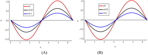
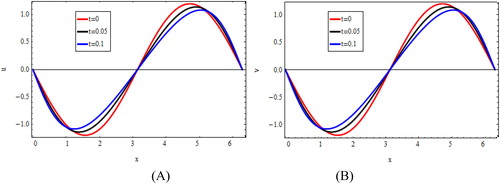
Figure 2. Approximate solutions of $u$ in (A) and $v$ in (B) for $k_{1} = - 2, k_{2} = 1,$ $k_{3} = 1, N = 200$ and $Δ t = k = 0.001$ at $t = 0, 0.05, 0.1 .$

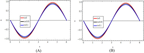
Figure 3. Exact and approximate solutions of $u$ in (A) and $v$ in (B) for $k_{1} = - 2, k_{2} = 1,$ $k_{3} = 1, N = 200$ and $Δ t = k = 0.001$ at $t = 0.1 .$

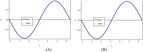
Figure 4. Approximate solutions of $u$ in (A) and $v$ in (B) for $k_{1} = - 2, k_{2} = 1,$ $k_{3} = 8, N = 200$ and $Δ t = k = 0.001$ at $t = 0, 0.05, 0.1 .$

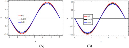
Figure 5. Approximate solutions of $u$ in (A) and $v$ in (B) for $k_{1} = - 2, k_{2} = 8,$ $k_{3} = 1, N = 200$ and $Δ t = k = 0.001$ at $t = 0, 0.05, 0.1 .$

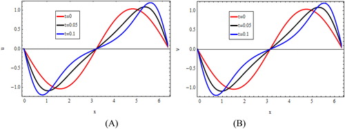
Figure 6. Approximate solutions of $u$ in (A) and $v$ in (B) for $k_{1} = 2, k_{2} = 1,$ $k_{3} = 1, N = 200$ and $Δ t = k = 0.001$ at $t = 0, 0.05, 0.1 .$

Test problem (2)

Numerical solutions of considered coupled Burgers' equations have been obtained for $k_{1} = 2$ with different values of $k_{2}$ and $k_{3}$ at different time levels. In this situation the exact solution is $\begin{matrix} u (x, t) = a_{0} - 2 A [\frac{2 k_{2} - 1}{4 k_{2} k_{3} - 1}] \tanh (A (x - 2 A t)), \\ v (x, t) = a_{0} [\frac{2 k_{3} - 1}{2 k_{2} - 1}] - 2 A [\frac{2 k_{2} - 1}{4 k_{2} k_{3} - 1}] \tanh (A (x - 2 A t)) . \end{matrix}$

The initial and boundary conditions are taken from the exact solution given below: $\begin{matrix} u (x, 0) = a_{0} - 2 A [\frac{2 k_{2} - 1}{4 k_{2} k_{3} - 1}] \tanh (A (x)), \\ v (x, 0) = a_{0} [\frac{2 k_{3} - 1}{2 k_{2} - 1}] - 2 A [\frac{2 k_{2} - 1}{4 k_{2} k_{3} - 1}] \tanh (A (x)), \end{matrix}$ where $a_{0} = 0.05$ and $A = \frac{1}{2} [\frac{a_{0} (4 k_{2} k_{3} - 1)}{2 k_{2} - 1}] .$ The numerical solutions for $u (x, t)$ and $v (x, t)$ have been computed for the domain $x \in [- 10, 10],$ $k = 0.01$ and number of partitions $N = 10,$ $N = 50,$ $N = 100$ and $N = 200 .$ $L_{2}$ and $L_{\infty}$ norms have been presented in for $t = 1, k_{1} = 2, k_{2} = 0.1$ and $k_{3} = 0.3 .$ and include comparison of our numerical results of problem (2) with results obtained from (Raslan et al., Citation2016) for the variables $u (x, t)$ and $v (x, t)$ with $a_{0} = 0.05,$ $N = 16,$ $k = 0.01$ at different time $t$ and different values of $k_{2}, k_{3} .$ and , contain comparison of our numerical results of problem (2) with results obtained from (Raslan et al., Citation2016) for the variables $u (x, t)$ and $v (x, t)$ with $a_{0} = 0.05,$ $N = 21,$ $k = 0.01$ at different values of $k_{2}, k_{3}$ and $t .$

Table 4. $L_{2}$ -norm and $L_{\infty}$ -norm for $t = 1,$ $k = 0.01$ at deferent values of $N$ $k_{1} = 2, k_{2} = 0.1$ and $k_{3} = 0.3 .$

Display Table

Table 5. Comparison between numerical results of problem (2) and results obtained from (Raslan et al., Citation2016) for the variable $u$ with $a_{0} = 0.05,$ $N = 16,$ $k = 0. 01.$

Display Table

Table 6. Comparison between numerical results of problem (2) and results obtained from (Raslan et al., Citation2016) for the variable $v$ with $a_{0} = 0.05,$ $N = 16,$ $k = 0.01 .$

Display Table

Table 7. Comparison between numerical results of problem (2) and results obtained from (Raslan et al., Citation2016) for the variable $u$ with $a_{0} = 0.05,$ $N = 21,$ $k_{1} = 2,$ $k = 0.01 .$

Display Table

Table 8. Comparison between numerical results of problem (2) and results obtained from (Raslan et al., Citation2016) for the variable $v$ with $a_{0} = 0.05,$ $N = 21,$ $k = 0.01 .$

Display Table

Table 9. $L_{2}$ - norm and $L_{\infty}$ -norm for $t = 1,$ $k = 0.01$ at deferent values of $N,$ $k_{1} = 2,$ $k_{2} = 0.1$ and $k_{3} = 0.3 .$

Display Table

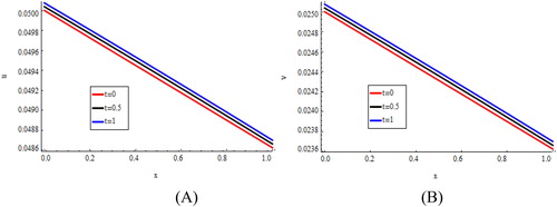
The corresponding graphical illustrations are presented in (), computed approximation solutions of $u (x, t)$ and $v (x, t)$ for $k_{1} = 2, k_{2} = 0.1,$ $k_{3} = 0.3, N = 200$ and $Δ t = k = 0.01$ at $t = 0, 0.5, 1, x \in [0, 1] .$

Figure 7. Approximate solutions of $u$ in (A) and $v$ in (B) for $k_{1} = 2, k_{2} = 1, k_{3} = 0.3,$ $N = 200$ and $Δ t = k = 0.01$ at $t = 0, 0.5, 1 .$

7. Conclusions

In this paper, a numerical scheme for the nonlinear coupled Burger's equations has been proposed using a collocation method based on septic B-spline functions. The proposed method is unconditionally stable. The method has been evaluated by two test problems. The accuracy of the method has been measured by computing $L_{2}$ and $L_{\infty}$ error norms. The obtained numerical results are quite satisfactory and comparable with the analytic solution and better than the obtained numerical results in (Raslan et al., Citation2016). Based on the stability and accuracy of the proposed method, the method can be extended to solve various linear and nonlinear partial differential equations.

Disclosure statement

No potential conflict of interest was reported by the authors.

References

Abdou, M. A., & Soliman, A. A. (2005). Variational iteration method for solving Burgers and coupled Burger equations. The Journal of Computational and Applied Mathematics, 181(2), 245–251.
Web of Science ®Google Scholar
Ali, K. K., Raslan, K. R., & El-Danaf, T. S. (2015). Non-polynomial spline method for solving coupled Burgers’ equations. Computational Methods for Differential Equations, 3(3), 218–230.
Web of Science ®Google Scholar
Bashan, A., Karakoc, S. B. G., & Geyikli, T. (2015). B-spline differential quadrature method for the modified Burgers' equation. Cankaya University Journal of Science and Engineering, 12(1), 1–13.
Google Scholar
Bonkile, M. P., Awasthi, A., Lakshmi, C., Mukundan, V., & Aswin, V. S. (2018). A systematic literature review of Burgers’ equation with recent advances. Pramana: Journal of Physics, 90, 69.
Web of Science ®Google Scholar
Bryan, R., Todd, O., Lee, M. K., & Robert, M. (2017). A mass-conserving mixed Fourier-Galerkin B-spline-collocation method for direct numerical simulation of the variable- density Navier-Stokes equations. APS Division of Fluid Dynamics, 2017, A32.006R.
Google Scholar
Burger, J. M. (1948). A mathematical model illustrating the theory of turbulence. Advances in Applied Mechanics, 1, 171–199.
Google Scholar
Cole, J. D. (1951). On a quasi linear parabolic equations occurring in aerodynamics. Quarterly of Applied Mathematics, 9(3), 225–236.
Web of Science ®Google Scholar
Deghan, M., Asgar, H., & Mohammad, S. (2007). The solution of coupled Burgers equations using Adomian-Pade technique. Appl. Math. Comput, 189(2), 1034–1047.
Web of Science ®Google Scholar
El-Danaf, T. S. (2008). Septic B-spline method of the Korteweg-de Vries-Burger’s equation. Communications in Nonlinear Science and Numerical Simulation, 13, 554–566.
Web of Science ®Google Scholar
Ersoy, O., & Dag, I. (2015, March 2). An exponential cubic B-spline finite element method for solving the nonlinear coupled Burger equation. arXiv:1503.00456 [Math NA].
Google Scholar
Esipov, S. E. (1995). Coupled Burger's equations-a model of polydispersive sedimentation. Physical Review. E, Statistical Physics, Plasmas, Fluids, and Related Interdisciplinary Topics, 52(4), 3711–3718.
PubMed Web of Science ®Google Scholar
Geyikli, T., & Karakoc, S. B. G. (2011). Septic B-spline collocation method for the numerical solution of the modified equal width wave equation. Applied Mathematics, 2(6), 739–749.
Google Scholar
Islam, S., Sarler, B., Vertnik, R., & Kosec, G. (2012). Radial basis function collocation method for the numerical solution of the two-dimensional transient nonlinear couple Burgers equations. Appl. Math. Model, 36(3), 1148–1160.
Web of Science ®Google Scholar
Karakoc, S. B. G., Bashan, A., & Geyikli, T. (2014). Two different methods for numerical solution of the Modified Burgers' equation. The Scientific World Journal, 2014, 780269.
Google Scholar
Karakoc, S. B. G., & Zeybek, H. (2016). Solitary-wave solutions of the GRLW equation using septic B-spline collocation method. Journal of Applied Mathematics and Computing, 289, 159–1571. doi:10.1016/j.amc.2016.05.021
Google Scholar
Kaya, D. (2001). An explicit solution of coupled viscous Burgers equations by the Decomposition method. Int. J. Math. Math. Sci, 27(11), 675–680. doi:10.1155/S0161171201010249
Google Scholar
Khater, A. H., Temsah, R. S., & Hassan, M. M. (2008). A Chebyshev spectral collocation method for solving Burgers-type equations. The Journal of Computational and Applied Mathematics, 222(2), 333–350.
Web of Science ®Google Scholar
Korkmaz, A., & Akmaz, H. K. (2015). Numerical simulations for transport of conservative pollutants. Selcuk Journal of Applied Mathematics, 16(1), 1–11.
Google Scholar
Korkmaz, A., & Akmaz, H. K. (2018). Numerical solution of non-conservative linear transport problem. TWMS Journal of Applied and Engineering Mathematics, 8(1a), 167–177.
Web of Science ®Google Scholar
Kutluay, S., & Ucar, Y. (2013). Numerical solutions of the coupled Burgers’ equation by the Galerkin quadratic B‐spline finite element method. Mathematical Methods in the Applied Sciences, 36(17), 2403–2415. doi:10.1002/mma.2767
Web of Science ®Google Scholar
Lashkarian, E., Hejazi, S. R., Habibi, N., & Motamednezhad, A. (2019). Symmetry properties, conservation laws, reduction and numerical approximations of time fractional cylindrical- Burger equation. Communications in Nonlinear Science and Numerical Simulation, 67, 176–191.
Web of Science ®Google Scholar
Luo, X. Q., Liu, L. B., Ouyang, A., & Long, G. (2018). B-spline collocation and self-adapting differential evolution (jDE) algorithm for a singularly perturbed convection–diffusion problem. Soft Computing, 22(8), 2683–2693.
Web of Science ®Google Scholar
Mittal, R. C., & Arora, G. (2011). Numerical solution of the coupled viscous Burgers’ equation. Communications in Nonlinear Science and Numerical Simulation, 16(3), 1304–1313.
Web of Science ®Google Scholar
Mokhtari, R., Toodar, A. S., & Chegini, N. G. (2011). Application of the generalized differential quadrature method in solving Burgers’ equations. Communications in Theoretical Physics, 56(6), 1009–1015.
Web of Science ®Google Scholar
Nee, J., & Duan, J. (1998). Limit set of trajectories of the coupled viscous Burgers’ equations. Applied Mathematics Letters, 11(1), 57–61.
Web of Science ®Google Scholar
Pana, K., Wu, X., Yue, X., & Ni, R. (2018). A spatial sixth-order CCD-TVD method for solving multidimensional coupled Burgers’ equation. arXiv:1805.08407v1 [Math NA].
Google Scholar
Prakasha, A., Kumar, M., & Sharma, K. K. (2015). Numerical method for solving fractional coupled Burgers equations. Journal of Applied Mathematics and Computing., 260, 314–320.
Google Scholar
Quarteroni, A., Sacco, R., & Saleri, F. (2007). Numerical mathematics. Berlin: Springer-Verlag.
Google Scholar
Ramadan, M. A., El- Danaf, T. S., & Abd Alaal, F. E. (2005). A numerical solution of the Burgers' equation using septic B-splines. Chaos Solitons & Fractals, 26, 795–804.
Web of Science ®Google Scholar
Rashid, A., & Ismail, A. I. (2009). A Fourier pseudo spectral method for solving coupled Viscous Burgers equations. Computational Methods in Applied Mathematics, 9(4), 412–420.
Google Scholar
Raslan, K. R., El-Danaf, T. S., & Ali, K. K. (2016). Collocation method with cubic trigonometric B-spline algorithm for solving coupled Burges' equations. Far East Journal of Applied Mathematics, 95(2), 109–123.
Google Scholar
Raslan, K. R., El-Danaf, T. S., & Ali, K. K. (2017). Collocation method with quintic B- spline method for solving coupled Burges' equations. Far East Journal of Applied Mathematics, 96(1), 55–75.
Google Scholar
Rubin, S. G., & Graves, R. A. (1975). Cubic spline approximation for problems in fluid mechanics. NASA TRR-436. Washington, DC: NASA.
Google Scholar
Rohila, R., & Mittal, R. C. (2018). Numerical study of reaction diffusion Fisher’s equation by fourth order cubic B-spline collocation method. Mathematical Sciences, 12(2), 79–89.
Web of Science ®Google Scholar
Sharifi, S., & Rashidinia, J. (2016). Numerical solution of hyperbolic telegraph equation by cubic B-spline collocation method. Journal of Applied Mathematics and Computing, 281, 28–38.
Google Scholar
Shi, F., Zheng, H., Cao, Y., Li, J., & Zhao, R. (2017). A fast numerical method for solving coupled Burgers’ equations. Numerical Methods for Partial Differential Equations, 33(6), 1823–1838.
Web of Science ®Google Scholar
Soliman, A. A. (2006). The modified extended tanh-function method for solving Burgers type equations. Journal of Physics A: Mathematical and Theoretical, 361(2), 394–404.
Google Scholar
Soliman, A. A., & Hussien, M. H. (2005). Collocation solution for RLW equation with septic spline. Journal of Applied Mathematics and Computing, 161, 623–636.
Google Scholar
Srivastava, V. K., Awasthi, M. K., Tamsir, M., & Singh, S. (2013). An implicit finite-difference solution to one dimensional coupled Burgers' equation. Asian-European Journal of Mathematics, 6(4), 1350058.
Google Scholar
Srivastava, V. K., Awasthi, M. K., & Tamsir, M. (2013). A fully implicit finite-difference solution to one dimensional coupled nonlinear Burgers equation. International Journal of Computing Science and Mathematics, 7(4), 283–288.
Google Scholar
Srivastava, V. K., Tamsir, M., Awasthi, M. K., & Singh, S. (2014). One-dimensional coupled Burgers' equation and its numerical solution by an implicit logarithmic finite-difference method. AIP Advances, 4(3), 037119.
Web of Science ®Google Scholar
Wang, G. W., & Kara, A. H. (2018). Group analysis, fractional explicit solutions and conservation laws of time fractional generalized Burgers’ equation. Communications in Theoretical Physics, 69(1), 5–8.
Web of Science ®Google Scholar
Wei, G. W., & Gu, Y. (2002). Conjugate filter approach for solving Burgers’ equation. The Journal of Computational and Applied Mathematics, 149(2), 439–456.
Web of Science ®Google Scholar

Septic B-spline collocation method for numerical solution of the coupled Burgers’ equations

Abstract

1. Introduction

2. Septic B-spline collocation method

3. Solution of coupled burger equations

4. Initial values

5. Stability analysis of the method

6. Numerical tests and results of coupled burgers' equations

Table 1. $L_{2}$ -norm and $L_{\infty}$ -norm for $t = 0.1,$ $k = 0.001$ at deferent $N .$

Table 2. $L_{2}$ -norm and $L_{\infty}$ -norm for $t = 1,$ $k = 0.01, 0.001$ when $N = 200 .$

Table 3. Comparison between numerical results of problem (1) and results obtained from (Raslan et al., Citation2016) for the variable $u$ and $v$ with, $N = 50,$ $k = 0. 01.$

Table 4. $L_{2}$ -norm and $L_{\infty}$ -norm for $t = 1,$ $k = 0.01$ at deferent values of $N$ $k_{1} = 2, k_{2} = 0.1$ and $k_{3} = 0.3 .$

Table 5. Comparison between numerical results of problem (2) and results obtained from (Raslan et al., Citation2016) for the variable $u$ with $a_{0} = 0.05,$ $N = 16,$ $k = 0. 01.$

Table 6. Comparison between numerical results of problem (2) and results obtained from (Raslan et al., Citation2016) for the variable $v$ with $a_{0} = 0.05,$ $N = 16,$ $k = 0.01 .$

Table 7. Comparison between numerical results of problem (2) and results obtained from (Raslan et al., Citation2016) for the variable $u$ with $a_{0} = 0.05,$ $N = 21,$ $k_{1} = 2,$ $k = 0.01 .$

Table 8. Comparison between numerical results of problem (2) and results obtained from (Raslan et al., Citation2016) for the variable $v$ with $a_{0} = 0.05,$ $N = 21,$ $k = 0.01 .$

Table 9. $L_{2}$ - norm and $L_{\infty}$ -norm for $t = 1,$ $k = 0.01$ at deferent values of $N,$ $k_{1} = 2,$ $k_{2} = 0.1$ and $k_{3} = 0.3 .$

7. Conclusions

Disclosure statement

Related Research Data

References

Information for

Open access

Opportunities

Help and information

Septic B-spline collocation method for numerical solution of the coupled Burgers’ equations

Abstract

1. Introduction

2. Septic B-spline collocation method

3. Solution of coupled burger equations

4. Initial values

5. Stability analysis of the method

6. Numerical tests and results of coupled burgers' equations

Table 1. L2-norm and L∞-norm for t=0.1, k=0.001 at deferent N.

Table 2. L2-norm and L∞-norm for t=1, k=0.01, 0.001 when N=200.

Table 3. Comparison between numerical results of problem (1) and results obtained from (Raslan et al., Citation2016) for the variable u and v with, N=50, k=0.01.

Table 4. L2-norm and L∞-norm for t=1, k=0.01 at deferent values of N k1=2, k2=0.1 and k3=0.3.

Table 5. Comparison between numerical results of problem (2) and results obtained from (Raslan et al., Citation2016) for the variable u with a0=0.05, N=16, k=0.01.

Table 6. Comparison between numerical results of problem (2) and results obtained from (Raslan et al., Citation2016) for the variable v with a0=0.05, N=16, k=0.01.

Table 7. Comparison between numerical results of problem (2) and results obtained from (Raslan et al., Citation2016) for the variable uwitha0=0.05, N=21, k1=2, k=0.01.

Table 8. Comparison between numerical results of problem (2) and results obtained from (Raslan et al., Citation2016) for the variable v with a0=0.05, N=21, k=0.01.

Table 9. L2- norm and L∞-norm for t=1, k=0.01 at deferent values of N, k1=2, k2=0.1and k3=0.3.

7. Conclusions

Disclosure statement

Related Research Data

References

Related research

To cite this article:

Download citation

Your download is now in progress and you may close this window

Login or register to access this feature

Information for

Open access

Opportunities

Help and information

Keep up to date

Table 1. $L_{2}$ -norm and $L_{\infty}$ -norm for $t = 0.1,$ $k = 0.001$ at deferent $N .$

Table 2. $L_{2}$ -norm and $L_{\infty}$ -norm for $t = 1,$ $k = 0.01, 0.001$ when $N = 200 .$

Table 3. Comparison between numerical results of problem (1) and results obtained from (Raslan et al., Citation2016) for the variable $u$ and $v$ with, $N = 50,$ $k = 0. 01.$

Table 4. $L_{2}$ -norm and $L_{\infty}$ -norm for $t = 1,$ $k = 0.01$ at deferent values of $N$ $k_{1} = 2, k_{2} = 0.1$ and $k_{3} = 0.3 .$

Table 5. Comparison between numerical results of problem (2) and results obtained from (Raslan et al., Citation2016) for the variable $u$ with $a_{0} = 0.05,$ $N = 16,$ $k = 0. 01.$

Table 6. Comparison between numerical results of problem (2) and results obtained from (Raslan et al., Citation2016) for the variable $v$ with $a_{0} = 0.05,$ $N = 16,$ $k = 0.01 .$

Table 7. Comparison between numerical results of problem (2) and results obtained from (Raslan et al., Citation2016) for the variable $u$ with $a_{0} = 0.05,$ $N = 21,$ $k_{1} = 2,$ $k = 0.01 .$

Table 8. Comparison between numerical results of problem (2) and results obtained from (Raslan et al., Citation2016) for the variable $v$ with $a_{0} = 0.05,$ $N = 21,$ $k = 0.01 .$

Table 9. $L_{2}$ - norm and $L_{\infty}$ -norm for $t = 1,$ $k = 0.01$ at deferent values of $N,$ $k_{1} = 2,$ $k_{2} = 0.1$ and $k_{3} = 0.3 .$