A new convolution variational boundary element technique for design sensitivity analysis and topology optimization of anisotropic thermo-poroelastic structures

Abstract

The main objective of this paper is to propose a new efficient time domain boundary element technique for design sensitivity analysis and topology optimization of anisotropic thermo-poroelastic structures. The spatial regularization scheme based on integration by parts is performed in Laplace domain in conjunction with time-domain convolution variational boundary element method (CVBEM). The generating optimization problem is solved using the Moving Asymptotes Method (MAM) with the adjoint variable method to obtain optimal material distribution, influence of anisotropy on the thermo-poroelastic stresses sensitivities. The results from the numerical model demonstrate the validity, efficiency and accuracy of the proposed technique.

Keywords:

• Topology optimization
• convolution variational boundary element method
• moving asymptotes method
• anisotropy
• thermo-poroelasticity

1. Introduction

Exact (Mohyud-Din, Irshad, Ahmed, & Khan, 2017; Sun & Chen, 2018), fractional (Khan, Ellahi, Khan, & Mohyud-Din, 2017), optimal (Sikander, Khan, Ahmed, & Mohyud-Din, 2017; Sikander, Khan, & Mohyud-Din, 2017) and numerical (Abd-Alla, El-Naggar, & Fahmy, 2003; Abd-Alla, Fahmy, & El-Shahat, 2008;; El-Naggar, Abd-Alla, & Fahmy, 2003; Fahmy, 2008; Fahmy & El-Shahat, 2008; Iqbal, Mohyud-Din, & Bin-Mohsin, 2016; Mohamed, 2019; Mohyud-Din, Noor, & Noor, 2009; Mohyud‐Din, Yıldırım, & Sarıaydın, 2011; Shakeel & Mohyud-Din, 2015) solutions have been implemented in various physical problems. Topology optimization is a numerical design method which optimizes material distribution in a design domain under given loads, boundary conditions and constraints. It has been successfully implemented to various multiphysics problems (Bendsoe & Sigmund, 2004; Deaton & Grandhi, 2014). There are a lot of developed topology optimization methods such as density distribution (Zhou & Rozvany, 1991), level set (Wang, Wang, & Guo, 2003), topological derivative (Suresh, 2013)), phase field (Bourdin & Chambolle, 2003), and evolutionary methods (Xie & Steven, 1993). In the past few years, finite element (Koga, Lopes, Nova, de Lima, & Silva, 2013; Matsumori, Kondoh, Kawamoto, & Nomura, 2013; Qian & Dede, 2016; Yaji, Yamada, Kubo, Izui, & Nishiwaki, 2015) and Finite volume (Marck, Nemer, & Harion, 2013; Kontoleontos, Papoutsis-Kiachagias, Zymaris, Papadimitriou, & Giannakoglou, 2013; Martins & Hwang, 2013) methods have been used in topology optimization for solving coupled thermal-fluid problems. Also, discrete and continuous adjoint approaches have been used in topology optimization to solve sensitivity problems (Nadarajah & Jameson, 2000; Giles & Pierce, 2000; Gunzburger, 2003; Hinze, Pinnau, Ulbrich, & Ulbrich, 2009).

Understanding the effects and behavior of the elastic stress wave propagation is very important in the design of many engineering optimization problems. Analytical solutions are very difficult or even impossible to achieve. Therefore, the problem can be solved approximately by numerical methods which has been developed and successfully implemented the boundary element method to solve a wide range of general elastic problems. The boundary element method (BEM) ( Domínguez, 1993; Fahmy, 2011, 2012a, 2012b, 2012c, 2012d, 2012e, 2013a, 2013b, 2013c, 2017a, 2017b, 2018a, 2018b, 2018c, 2019a, 2019b, 2019c, 2019d, 2019e ) has been developed and successfully implemented to solve our current complex problem. Generally, Laplace-domain fundamental solutions are easier to obtain than time-domain fundamental solutions for engineering and scientific problems (Wang & Achenbach, 1994, 1995). consequently, the CVBEM is very useful for problems where time-domain fundamental solutions are not known, because it utilizes the Laplace-domain fundamental solutions of the governing equations of the problem. So, CVBEM expands the range of engineering problems that can be solved with the classical time-domain BEM.

The aim of this article is to develop a novel methodology for solving thermo-poroelastic topology optimization problems. The spatial regularization procedure based on integration by parts is performed in Laplace domain in conjunction with the time-domain convolution variational boundary element method (CVBEM). The spatial discretization is performed using the collocation scheme. An implicit differentiation method has been used to compute the temperature, displacements and pore pressure sensitivities with respect to the control variables. The adjoint variable method has been used to calculate sensitivities for objective function and constraints to allow for Moving Asymptotes Method (MAM) to solve the resulting topology optimization problem and find the optimal material distribution and influence of anisotropy on the optimal design.

The effects of anisotropy on the thermo-poroelastic stresses sensitivities are very pronounced. The optimum design of an elliptical sandwich structure has been considered to demonstrate the validity, efficiency and accuracy of the proposed technique.

2. Formulation of the problem

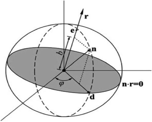
First, we consider the region $\mathrm{\Omega }=\left\{\left({\mathrm{x}}_1,\mathrm{}{\mathrm{x}}_2,\mathrm{}{\mathrm{x}}_3\right):0<{\mathrm{x}}_1<\underset{¯}{\alpha },\mathrm{}0<{\mathrm{x}}_2<\underset{¯}{\beta },\mathrm{}0<{\mathrm{x}}_3<\underset{¯}{\mathrm{\gamma }}\right\}$ with boundary $\mathrm{\Gamma }$ as shown in Figure 1.

Figure 1. Geometry of the fundamental solution integration.

According to Biot (1956a, 1956b) and Schanz (2001), the governing equations of anisotropic thermo-poroelastic structures can be described as (1) $${\left({\nabla }^T\sigma \right)}^T+F=\rho \ddot{u}+\varphi {\rho }_f\left({\ddot{u}}_f-\ddot{u}\right),\mathrm{}$$(1) (2) $$\dot{\zeta }+{\nabla }^{T}q=0,\mathrm{}$$(2) (3) $$\sigma =\left(C_{\mathit{ajlg}}\text{tr}ϵ-Ap\right)I-\mathfrak{B}\mathrm{}\theta ,\mathrm{}ϵ=\frac{1}{2}\left(\nabla u^T\mathrm{}+{\left(\nabla u^T\right)}^T\right),\mathrm{}$$(3) (4) $$\zeta =A\text{tr}ϵ+\frac{{\varphi }^2}{R}P,\mathrm{}$$(4) (5) $$q=-K\left(\nabla \mathrm{}p+{\rho }_f\ddot{u}+\frac{{\rho }_a+\varphi {\rho }_f}{\varphi }\left({\ddot{u}}_f-\ddot{u}\right)\right),\mathrm{}$$(5) (6) $${\mathrm{k}}_{pj}{\theta }_{,pj}=c\rho \dot{\theta }-\rho \mathfrak{X}.\mathrm{}$$(6)

According to Fourier's law, the heat flux ${\mathcal{q}}_p$ is defined by (7) $${\mathcal{q}}_p=-k_{pj}{\theta }_{,j}.\mathrm{}$$(7) where $\sigma$ is the total stress tensor, $ϵ$ is the linear strain tensor, $C_{\mathit{ajlg}}$ is the constant elastic moduli, $\rho ={\rho }_s\left(1-\varphi \right)+\varphi {\rho }_f$ is the bulk density, ${\rho }_s$ is the solid density, ${\rho }_f$ is the fluid density, $u$ is the displacement field in the solid, $u_f$ is the displacement field in the fluid, $\theta$ is the temperature, $\mathfrak{B}$ are stress-temperature coefficients, $q$ is the fluid-specific flux, $F$ are the total body forces, $\mathrm{tr}$ denotes the trace, $A=\mathrm{}\varphi \left(1+Q/R\right)$ is Biot’s effective stress coefficient, $Q$ and $R$ are the solid-fluid coupling parameters, $p$ is the pore pressure, $\zeta$ is the fluid volume variation measured in unit reference volume, $\varphi =\frac{V^f}{V}$ is the porosity, $V^f$ is the fluid volume, $V=V^f+V^s$ is the total volume (bulk volume), $V^s$ is the solid volume, $\tau$ is the time, $K$ is the permeability, ${\rho }_a=\mathbb{C}\varphi {\rho }_f$ (Bonnet & Auriault, 1985).

The equations of motion which describe our problem can be written in matrix form as follows (Bonnet, 1987; Messner & Schanz, 2011) (8) $$\left.\begin{array}{c}{\widehat{B}}_{\tilde{x}}{\widehat{u}}^g\left(\tilde{x}\right)=0\text{for}\tilde{x}\in \mathrm{\Omega }\mathrm{}\\ {\widehat{u}}^g\left(x\right)={\widehat{g}}_D\text{for}x\in {\Gamma }_D\\ {\widehat{t}}^g\left(x\right)={\widehat{g}}_N\text{for}x\in {\Gamma }_N\end{array}\right\}\mathrm{}$$(8)

where the operator ${\widehat{B}}_{\tilde{x}}$ and the tractions ${\widehat{t}}^g$ are defined as (9) $${\widehat{B}}_{\tilde{x}}=\left[\begin{array}{ccc}{B}_{\tilde{x}}^e+s^2\left(\rho -\beta {\rho }_f\right)I& \left(\alpha -\beta \right){\nabla }_{\tilde{x}}& -\mathfrak{B}{\nabla }_{\tilde{x}}\\ s\left(\alpha -\beta \right){\nabla }_{\tilde{x}}^T& -\mathrm{}\frac{\beta }{s{\rho }_f}{\Delta }_{\tilde{x}}+\frac{{s\varphi }^2}{R}& 0\end{array}\right],\mathrm{}$$(9) (10) $${\widehat{t}}^g\left(x\right)=\mathrm{}\left[\begin{array}{ccc}{T}_x^e& -\alpha n_x& 0\\ s\beta n_x^T& \frac{\beta }{s{\rho }_f}{n}_x^T{\nabla }_x& 0\end{array}\right]\left[\begin{array}{c}\widehat{u}\left(x\right)\\ \widehat{p}\left(x\right)\\ \theta \left(x\right)\end{array}\right].\mathrm{}$$(10) $\text{In which}\beta =\frac{{\varphi }^{2}sK{\rho }_f}{{\varphi }^2+sK({\rho }_a+\varphi {\rho }_f)}$

where $B_{\tilde{x}}^e$ is the linear elastostatics operator and $T_x^e$ is the traction derivative with respect to $x.$ The thermo-poroelastic medium occupies the region $\mathrm{\Omega }$ that bounded by a closed curve $\Gamma$ that is subdivided into two non-intersective parts ${\Gamma }_D$ and ${\Gamma }_N.$ The Dirichlet boundary condition relates the datum ${\widehat{g}}_D$ to the displacement on the ${\Gamma }_D$ and the Neumann boundary condition relates the datum ${\widehat{g}}_N$ to the surface traction on the ${\Gamma }_N.$

3. Boundary element implementation for the temperature field

Using the boundary element method as described in Fahmy (2012a), we obtain (11) $$\theta \left(\xi \right)={\int }_{\Gamma }^{}\left({\mathcal{q}}^{\mathrm{\ast }}\theta -{\theta }^{\mathrm{\ast }}\mathcal{q}\right)d\mathrm{C}-{\int }_{\mathrm{\Omega }}^{}\left(c\rho \dot{\theta }-\rho \mathfrak{X}\right){\theta }^{\mathrm{\ast }}\mathrm{d}\mathrm{R}.\mathrm{}$$(11)

The source term in (11(11) $$\theta \left(\xi \right)={\int }_{\Gamma }^{}\left({\mathcal{q}}^{\mathrm{\ast }}\theta -{\theta }^{\mathrm{\ast }}\mathcal{q}\right)d\mathrm{C}-{\int }_{\mathrm{\Omega }}^{}\left(c\rho \dot{\theta }-\rho \mathfrak{X}\right){\theta }^{\mathrm{\ast }}\mathrm{d}\mathrm{R}.\mathrm{}$$(11) ) has been approximated using a series $f^q$ and coefficients ${\overline{\alpha }}^q\mathrm{}$ as (12) $${\int }_{\mathrm{\Omega }}^{}\left(c\rho \dot{\theta }-\rho \mathfrak{X}\right){\theta }^{\mathrm{\ast }}\mathrm{d}\mathrm{R}\approx \sum _{q=1}^N{\overline{\alpha }}^q{\int }_{\mathrm{\Omega }}^{}{f}^q{\theta }^{\mathrm{\ast }}\mathrm{d}\mathrm{R}.\mathrm{}$$(12)

Thus, the representation formula can be expressed as (13) $$\theta \left(\xi \right)+{\int }_{\Gamma }^{}\left({\theta }^{\mathrm{\ast }}\mathcal{q}-{\mathcal{q}}^{\mathrm{\ast }}\theta \right)d\mathrm{C}=\sum _{\mathrm{q}=1}^{\mathrm{N}}\left({\theta }^q\left(\xi \right)+{\int }_{\Gamma }^{}\left({\theta }^{\mathrm{\ast }}{\mathcal{q}}^q-{\mathcal{q}}^{\mathrm{\ast }}{\theta }^q\right)d\Gamma \right){\overline{\alpha }}^q.\mathrm{}$$(13)

The temperature $T$ and the heat flux $q$ and their corresponding particular solutions $T^q$ and$\mathrm{}{q}^q\mathrm{}$ can be approximated as (14) $$\left\{\theta ,\mathcal{}\mathcal{q}\right\}\approx \sum _{k=1}^N{\overline{\phi }}_k\left\{{\check{\theta }}_k,\mathrm{}{\check{\mathcal{q}}}_k\right\}={\overline{\mathrm{\Phi }}}^T\left\{\check{\theta },\mathrm{}\check{\mathcal{q}}\right\},\mathrm{}\left\{T^{\mathcal{q}},\mathrm{}{\mathcal{q}}^{\mathcal{q}}\right\}\approx \sum _{k=1}^N{\overline{\phi }}_k\left\{{\check{\theta }}_k^{\mathcal{q}},\mathrm{}{\check{\mathcal{q}}}_k^{\mathcal{q}}\right\}={\overline{\mathrm{\Phi }}}^T\left\{{\check{\theta }}^{\mathcal{q}},\mathrm{}{\check{\mathcal{q}}}^{\mathcal{q}}\right\}.\mathrm{}$$(14)

where $\check{\theta },$ $\check{\mathcal{q}},$ ${\check{\theta }}^{\mathcal{q}},$ ${\check{\mathcal{q}}}^{\mathcal{q}}$ and $\overline{\mathrm{\Phi }}$ are matrices.

By implementing point collocation procedure to (13(13) $$\theta \left(\xi \right)+{\int }_{\Gamma }^{}\left({\theta }^{\mathrm{\ast }}\mathcal{q}-{\mathcal{q}}^{\mathrm{\ast }}\theta \right)d\mathrm{C}=\sum _{\mathrm{q}=1}^{\mathrm{N}}\left({\theta }^q\left(\xi \right)+{\int }_{\Gamma }^{}\left({\theta }^{\mathrm{\ast }}{\mathcal{q}}^q-{\mathcal{q}}^{\mathrm{\ast }}{\theta }^q\right)d\Gamma \right){\overline{\alpha }}^q.\mathrm{}$$(13) ) and using (14(14) $$\left\{\theta ,\mathcal{}\mathcal{q}\right\}\approx \sum _{k=1}^N{\overline{\phi }}_k\left\{{\check{\theta }}_k,\mathrm{}{\check{\mathcal{q}}}_k\right\}={\overline{\mathrm{\Phi }}}^T\left\{\check{\theta },\mathrm{}\check{\mathcal{q}}\right\},\mathrm{}\left\{T^{\mathcal{q}},\mathrm{}{\mathcal{q}}^{\mathcal{q}}\right\}\approx \sum _{k=1}^N{\overline{\phi }}_k\left\{{\check{\theta }}_k^{\mathcal{q}},\mathrm{}{\check{\mathcal{q}}}_k^{\mathcal{q}}\right\}={\overline{\mathrm{\Phi }}}^T\left\{{\check{\theta }}^{\mathcal{q}},\mathrm{}{\check{\mathcal{q}}}^{\mathcal{q}}\right\}.\mathrm{}$$(14) ), we obtain the following system (15) $$\overline{\zeta }\check{\theta }-\overline{\eta }\check{\mathcal{q}}=\sum _{q=1}^N\left(\overline{\zeta }{\check{\theta }}^{\mathcal{q}}-\overline{\eta }{\check{\mathcal{q}}}^{\mathcal{q}}\right){\overline{\alpha }}^{\mathcal{q}}.\mathrm{}$$(15)

Let (16) $$\check{\mathbf{\Theta }}=\left[{\check{\mathrm{\Theta }}}^1\mathrm{}{\check{\mathrm{\Theta }}}^2\mathrm{}\dots {\check{\mathrm{\Theta }}}^N\right],\mathrm{}\check{\overline{\mathrm{\wp }}}=\left[{\check{q}}^1\mathrm{}{\check{q}}^2\mathrm{}\dots {\check{q}}^N\right],\mathrm{}\overline{\alpha }={\left[{\overline{\alpha }}^1\mathrm{}{\overline{\alpha }}^2\mathrm{}\dots {\overline{\alpha }}^N\right]}^T.\mathrm{}$$(16)

Using (16(16) $$\check{\mathbf{\Theta }}=\left[{\check{\mathrm{\Theta }}}^1\mathrm{}{\check{\mathrm{\Theta }}}^2\mathrm{}\dots {\check{\mathrm{\Theta }}}^N\right],\mathrm{}\check{\overline{\mathrm{\wp }}}=\left[{\check{q}}^1\mathrm{}{\check{q}}^2\mathrm{}\dots {\check{q}}^N\right],\mathrm{}\overline{\alpha }={\left[{\overline{\alpha }}^1\mathrm{}{\overline{\alpha }}^2\mathrm{}\dots {\overline{\alpha }}^N\right]}^T.\mathrm{}$$(16) ) into (15(15) $$\overline{\zeta }\check{\theta }-\overline{\eta }\check{\mathcal{q}}=\sum _{q=1}^N\left(\overline{\zeta }{\check{\theta }}^{\mathcal{q}}-\overline{\eta }{\check{\mathcal{q}}}^{\mathcal{q}}\right){\overline{\alpha }}^{\mathcal{q}}.\mathrm{}$$(15) ) we have (17) $$\overline{\zeta }\check{\theta }-\overline{\eta }\check{\mathcal{q}}=\left(\overline{\zeta }\check{\mathbf{\Theta }}-\overline{\eta }\check{\overline{\mathrm{\wp }}}\right)\overline{\alpha .}\mathrm{}$$(17)

By implementing a point collocation procedure to Eq. (16(16) $$\check{\mathbf{\Theta }}=\left[{\check{\mathrm{\Theta }}}^1\mathrm{}{\check{\mathrm{\Theta }}}^2\mathrm{}\dots {\check{\mathrm{\Theta }}}^N\right],\mathrm{}\check{\overline{\mathrm{\wp }}}=\left[{\check{q}}^1\mathrm{}{\check{q}}^2\mathrm{}\dots {\check{q}}^N\right],\mathrm{}\overline{\alpha }={\left[{\overline{\alpha }}^1\mathrm{}{\overline{\alpha }}^2\mathrm{}\dots {\overline{\alpha }}^N\right]}^T.\mathrm{}$$(16) ) as in Fahmy (2012a), we get (18) $$c\rho \check{\stackrel{̇}{\theta }}-\rho \check{r}=\overline{F}\overline{\alpha }\left(\tau \right).\mathrm{}$$(18)

From Eq. (18(18) $$c\rho \check{\stackrel{̇}{\theta }}-\rho \check{r}=\overline{F}\overline{\alpha }\left(\tau \right).\mathrm{}$$(18) ) the following expression can be derived (19) $$\overline{\alpha }\left(\tau \right)={\overline{F}}^{-1}\left(c\rho \check{\stackrel{̇}{\theta }}-\rho \check{r}\right).\mathrm{}$$(19)

Which can be substituted into (17(17) $$\overline{\zeta }\check{\theta }-\overline{\eta }\check{\mathcal{q}}=\left(\overline{\zeta }\check{\mathbf{\Theta }}-\overline{\eta }\check{\overline{\mathrm{\wp }}}\right)\overline{\alpha .}\mathrm{}$$(17) ) producing (20) $$\overline{\mathcal{M}}\check{\stackrel{̇}{\theta }}\left(\tau \right)+\overline{\zeta }\check{\theta }\left(\tau \right)=\overline{\eta }\check{\mathcal{q}}\left(\tau \right)+\check{\mathrm{\&Beta;}}\left(\tau \right).\mathrm{}$$(20) where (21) $$\overline{\mathcal{M}}=c\rho \upsilon ,\mathrm{}\check{\mathrm{\&Beta;}}=\rho \upsilon \check{r},\mathrm{}\upsilon =-\left(\overline{\zeta }\check{\theta }-\overline{\eta }\check{\overline{\mathrm{\wp }}}\right){\overline{F}}^{-1}.\mathrm{}$$(21)

The nodal vectors are subdivided into known $k$ and unknown $u$ superscripts (22) $$\left\{{\check{\theta }}^k,\mathrm{}{\check{\mathcal{q}}}^u\right\}\in {\mathrm{C}}_1,\mathrm{}\left\{{\check{\theta }}^u,\mathrm{}{\check{\mathcal{q}}}^k\right\}\in {\mathrm{C}}_2.\mathrm{}$$(22)

Thus, from (20(20) $$\overline{\mathcal{M}}\check{\stackrel{̇}{\theta }}\left(\tau \right)+\overline{\zeta }\check{\theta }\left(\tau \right)=\overline{\eta }\check{\mathcal{q}}\left(\tau \right)+\check{\mathrm{\&Beta;}}\left(\tau \right).\mathrm{}$$(20) ) we obtain the following matrix equation (23) $$\left[\begin{array}{cc}{\overline{\mathcal{M}}}^{11}& {\overline{\mathcal{M}}}^{12}\\ {\overline{\mathcal{M}}}^{21}& {\overline{\mathcal{M}}}^{22}\end{array}\right]\left[\begin{array}{c}{\check{\stackrel{̇}{\theta }}}^k\left(\tau \right)\\ {\check{\stackrel{̇}{\theta }}}^u\left(\tau \right)\end{array}\right]+\left[\begin{array}{cc}{\overline{\zeta }}^{11}& {\overline{\zeta }}^{12}\\ {\overline{\zeta }}^{21}& {\overline{\zeta }}^{22}\end{array}\right]\left[\begin{array}{c}{\check{\theta }}^k\left(\tau \right)\\ {\check{\theta }}^u\left(\tau \right)\end{array}\right]=\left[\begin{array}{cc}{\overline{\eta }}^{11}& {\overline{\eta }}^{12}\\ {\overline{\eta }}^{21}& {\overline{\eta }}^{22}\end{array}\right]\left[\begin{array}{c}{\check{\mathcal{q}}}^k\left(\tau \right)\\ {\check{\mathcal{q}}}^u\left(\tau \right)\end{array}\right]+\left[\begin{array}{c}{\check{B}}^1\left(\tau \right)\\ {\check{B}}^2\left(\tau \right)\end{array}\right].\mathrm{}$$(23)

Making use of (23(23) $$\left[\begin{array}{cc}{\overline{\mathcal{M}}}^{11}& {\overline{\mathcal{M}}}^{12}\\ {\overline{\mathcal{M}}}^{21}& {\overline{\mathcal{M}}}^{22}\end{array}\right]\left[\begin{array}{c}{\check{\stackrel{̇}{\theta }}}^k\left(\tau \right)\\ {\check{\stackrel{̇}{\theta }}}^u\left(\tau \right)\end{array}\right]+\left[\begin{array}{cc}{\overline{\zeta }}^{11}& {\overline{\zeta }}^{12}\\ {\overline{\zeta }}^{21}& {\overline{\zeta }}^{22}\end{array}\right]\left[\begin{array}{c}{\check{\theta }}^k\left(\tau \right)\\ {\check{\theta }}^u\left(\tau \right)\end{array}\right]=\left[\begin{array}{cc}{\overline{\eta }}^{11}& {\overline{\eta }}^{12}\\ {\overline{\eta }}^{21}& {\overline{\eta }}^{22}\end{array}\right]\left[\begin{array}{c}{\check{\mathcal{q}}}^k\left(\tau \right)\\ {\check{\mathcal{q}}}^u\left(\tau \right)\end{array}\right]+\left[\begin{array}{c}{\check{B}}^1\left(\tau \right)\\ {\check{B}}^2\left(\tau \right)\end{array}\right].\mathrm{}$$(23) ), the unknown fluxes ${\check{q}}^u(t)$ can be written as (24) $${\check{\mathcal{q}}}^u\left(\tau \right)={\left({\overline{\eta }}^{12}\right)}^{-1}[{\overline{\mathcal{M}}}^{11}{\check{\stackrel{̇}{\theta }}}^k\left(\tau \right)+{\overline{\mathcal{M}}}^{12}{\check{\stackrel{̇}{\theta }}}^u\left(\tau \right)+{\overline{\zeta }}^{11}{\check{\theta }}^k\left(\tau \right)+{\overline{\zeta }}^{12}{\check{\theta }}^u\left(\tau \right)-{\overline{\eta }}^{11}{\check{\mathcal{q}}}^k\left(\tau \right)-{\check{B}}^1\left(\tau \right)]$$(24)

Using (24(24) $${\check{\mathcal{q}}}^u\left(\tau \right)={\left({\overline{\eta }}^{12}\right)}^{-1}[{\overline{\mathcal{M}}}^{11}{\check{\stackrel{̇}{\theta }}}^k\left(\tau \right)+{\overline{\mathcal{M}}}^{12}{\check{\stackrel{̇}{\theta }}}^u\left(\tau \right)+{\overline{\zeta }}^{11}{\check{\theta }}^k\left(\tau \right)+{\overline{\zeta }}^{12}{\check{\theta }}^u\left(\tau \right)-{\overline{\eta }}^{11}{\check{\mathcal{q}}}^k\left(\tau \right)-{\check{B}}^1\left(\tau \right)]$$(24) ), the second row of (23(23) $$\left[\begin{array}{cc}{\overline{\mathcal{M}}}^{11}& {\overline{\mathcal{M}}}^{12}\\ {\overline{\mathcal{M}}}^{21}& {\overline{\mathcal{M}}}^{22}\end{array}\right]\left[\begin{array}{c}{\check{\stackrel{̇}{\theta }}}^k\left(\tau \right)\\ {\check{\stackrel{̇}{\theta }}}^u\left(\tau \right)\end{array}\right]+\left[\begin{array}{cc}{\overline{\zeta }}^{11}& {\overline{\zeta }}^{12}\\ {\overline{\zeta }}^{21}& {\overline{\zeta }}^{22}\end{array}\right]\left[\begin{array}{c}{\check{\theta }}^k\left(\tau \right)\\ {\check{\theta }}^u\left(\tau \right)\end{array}\right]=\left[\begin{array}{cc}{\overline{\eta }}^{11}& {\overline{\eta }}^{12}\\ {\overline{\eta }}^{21}& {\overline{\eta }}^{22}\end{array}\right]\left[\begin{array}{c}{\check{\mathcal{q}}}^k\left(\tau \right)\\ {\check{\mathcal{q}}}^u\left(\tau \right)\end{array}\right]+\left[\begin{array}{c}{\check{B}}^1\left(\tau \right)\\ {\check{B}}^2\left(\tau \right)\end{array}\right].\mathrm{}$$(23) ) can be expressed as follows (25) $${\overline{\mathcal{M}}}^u{\check{\stackrel{̇}{\theta }}}^u\left(\tau \right)+{\overline{\zeta }}^u{\check{\theta }}^u\left(\tau \right)={\overline{Q}}^k\left(\tau \right).\mathrm{}$$(25) where $${\overline{Q}}^k\left(\tau \right)={\check{B}}^k\left(\tau \right)+{\overline{\eta }}^k{\check{\mathcal{q}}}^k\left(\tau \right)-{\overline{\mathcal{M}}}^k{\check{\stackrel{̇}{\theta }}}^k\left(\tau \right)-{\overline{\zeta }}^k{\check{\theta }}^k\left(\tau \right),{\overline{\mathcal{M}}}^u={\overline{\mathcal{M}}}^{22}-{\overline{\eta }}^{22}{\left({\overline{\eta }}^{12}\right)}^{-1}{\overline{\mathcal{M}}}^{12},{\overline{\zeta }}^u={\overline{\zeta }}^{22}-{\overline{\eta }}^{22}{\left({\overline{\eta }}^{12}\right)}^{-1}{\overline{\zeta }}^{12},{\check{B}}^k\left(\tau \right)=B^2\left(\tau \right)-{\overline{\eta }}^{22}{\left({\overline{\eta }}^{12}\right)}^{-1}{B}^1\left(\tau \right),{\overline{\eta }}^k={\overline{\eta }}^{21}-{\overline{\eta }}^{22}{\left({\overline{\eta }}^{12}\right)}^{-1}{\overline{\eta }}^{11},{\overline{\mathcal{M}}}^k={\overline{\mathcal{M}}}^{21}-{\overline{\eta }}^{22}{\left({\overline{\eta }}^{12}\right)}^{-1}{\overline{\mathcal{M}}}^{11},{\overline{\zeta }}^k={\overline{\zeta }}^{21}-{\overline{\eta }}^{22}{\left({\overline{\eta }}^{12}\right)}^{-1}{\overline{\zeta }}^{11}.$$

By using the finite difference method, we can write (25(25) $${\overline{\mathcal{M}}}^u{\check{\stackrel{̇}{\theta }}}^u\left(\tau \right)+{\overline{\zeta }}^u{\check{\theta }}^u\left(\tau \right)={\overline{Q}}^k\left(\tau \right).\mathrm{}$$(25) ) as (26) $${\overline{\varsigma }}^u{\check{\theta }}_{n+1}^u={\overline{\mathbb{Q}}}_{n+1}^k.\mathrm{}$$(26) where $${\overline{\mathbb{Q}}}_{n+1}^k={\overline{Q}}_{n+1}^k+\frac{{\overline{\mathcal{M}}}^u}{\Delta \tau }{\check{\theta }}_n^u,\mathrm{}{\overline{\varsigma }}^u=\frac{{\overline{\mathcal{M}}}^u}{\Delta \tau }+{\overline{\zeta }}^u.$$

4. BEM implementation for traction and displacement fields

According to problem (8(8) $$\left.\begin{array}{c}{\widehat{B}}_{\tilde{x}}{\widehat{u}}^g\left(\tilde{x}\right)=0\text{for}\tilde{x}\in \mathrm{\Omega }\mathrm{}\\ {\widehat{u}}^g\left(x\right)={\widehat{g}}_D\text{for}x\in {\Gamma }_D\\ {\widehat{t}}^g\left(x\right)={\widehat{g}}_N\text{for}x\in {\Gamma }_N\end{array}\right\}\mathrm{}$$(8) ), the representation formula of the unknown field ${\widehat{u}}^g$ can be described as (27) $${\widehat{u}}^g\left(\tilde{x}\right)={\left(\widehat{V}{\widehat{t}}^g\right)}_{\Omega }\left(\tilde{x}\right)-{\left(\widehat{K}{\widehat{u}}^g\right)}_{\Omega }\left(\tilde{x}\right)\text{for}\tilde{x}\in \mathit{\Omega }.\mathrm{}$$(27) where (28) $${\left(\widehat{V}{\widehat{t}}^g\right)}_{\Omega }\left(\tilde{x}\right)={\int }_{\mathrm{\Gamma }}^{}{\widehat{U}}^T\left(y-\tilde{x}\right){\widehat{t}}^g\left(y\right)d{s}_y,\mathrm{}$$(28) (29) $${\left(\widehat{K}{\widehat{u}}^g\right)}_{\Omega }\left(\tilde{x}\right)={\int }_{\mathrm{\Gamma }}^{}{\left({\widehat{T}}_y\widehat{U}\right)}^T\left(y-\tilde{x}\right){\widehat{u}}^g\left(y\right)d{s}_y.\mathrm{}$$(29)

Based on the anisotropic fundamental solutions of Wang and Achenbach (1994, 1995), we assumed that the fundamental solution $\widehat{U}\left(r\right)$ and the corresponding traction ${\widehat{T}}_y$ can be written in Laplace domain as follows (Messner & Schanz, 2011). (30) $$\widehat{U}\left(r\right)=\left[\begin{array}{ccc}{\widehat{U}}^s\left(r\right)& {\widehat{U}}^f\left(r\right)& 0\\ {\left({\widehat{P}}^s\right)}^T\left(r\right)& {\widehat{P}}^f\left(r\right)& 0\end{array}\right],\mathrm{}{\widehat{T}}_y=\left[\begin{array}{ccc}{T}_y^e& s\alpha n_y& 0\\ -\beta n_y^T& \frac{\beta }{s{\rho }^f}{n}_y^T\nabla & 0\end{array}\right]\text{with}r≔\left|y-x\right|.\mathrm{}$$(30)

where the solid displacement fundamental solution ${\widehat{U}}^s\left(r\right)$ can be expressed as (31) $${\widehat{U}}^s\left(r\right)=\frac{1}{4\pi r\left(\rho -\beta {\rho }^f\right)}[{\mathbb{R}}_1\frac{\left(k_4^2-k_2^2\right)}{\left(k_1^2-k_2^2\right)}{e}^{-k_{1}r}-{\mathbb{R}}_2\frac{\left(k_4^2-k_1^2\right)}{\left(k_1^2-k_2^2\right)}{e}^{-k_{2}r}+\left(I{k}_3^2-{\mathbb{R}}_3\right)e^{-k_{3}r}].\mathrm{}$$(31) with (32) $${\mathbb{R}}_j=\frac{3{\nabla }_{y}r{\nabla }_y^{T}r-I}{r^2}+k_j\frac{3{\nabla }_{y}r{\nabla }_y^{T}r-I}{r}+k_j^2{\nabla }_{y}r{\nabla }_y^{T}r.\mathrm{}$$(32)

Eq. (31(31) $${\widehat{U}}^s\left(r\right)=\frac{1}{4\pi r\left(\rho -\beta {\rho }^f\right)}[{\mathbb{R}}_1\frac{\left(k_4^2-k_2^2\right)}{\left(k_1^2-k_2^2\right)}{e}^{-k_{1}r}-{\mathbb{R}}_2\frac{\left(k_4^2-k_1^2\right)}{\left(k_1^2-k_2^2\right)}{e}^{-k_{2}r}+\left(I{k}_3^2-{\mathbb{R}}_3\right)e^{-k_{3}r}].\mathrm{}$$(31) ) can be written as (Schanz, 2001) (33) $${\widehat{U}}^s\left(r\right)=\frac{1}{4\pi \mu r\left(\lambda +2\mu \right)}\left[\left(\lambda +\mu \right){\nabla }_{y}r{\nabla }_y^{T}r+I\left(\lambda +3\mu \right)\right]+O\left(r^0\right).\mathrm{}$$(33)

According to the regularization procedure in this article, the solid displacement fundamental solution ${\widehat{U}}^s\left(r\right)$ can be divided into a singular part ${\widehat{U}}_s^s\left(r\right)$ plus a regular part ${\widehat{\mathrm{U}}}_{\mathrm{r}}^{\mathrm{s}}\left(\mathrm{r}\right)$ as $${\widehat{U}}^s\left(r\right)={\widehat{U}}_s^s\left(r\right)+{\widehat{U}}_r^s\left(r\right)\text{with}r≔\left|y-x\right|=\frac{1}{\mu }\left[I{\Delta }_y-\mathrm{}\frac{\lambda +\mu }{\lambda +2\mu }{\nabla }_y{\nabla }_y^T\right]{\Delta }_y\widehat{x}\left(r\right)$$ (34) $$-\frac{1}{\mu }[\left(\left(k_1^2+k_2^2\right){\Delta }_y-k_1^2{k}_2^2\right)I-\left(k_1^2+k_2^2-k_4^2-\frac{k_1^2{k}_2^2}{k_3^2}\right){\nabla }_y{\nabla }_y^T]\widehat{x}\left(r\right).\mathrm{}$$(34) where $$\widehat{x}\left(r\right)=\frac{1}{4\pi r}[\frac{e^{-k_{1}r}}{\left(k_2^2-k_1^2\right)\left(k_3^2-k_1^2\right)}+\frac{e^{-k_{2}r}}{\left(k_2^2-k_1^2\right)\left(k_2^2-k_3^2\right)}+\frac{e^{-k_{3}r}}{\left(k_1^2-k_3^2\right)\left(k_2^2-k_3^2\right)}]$$ (35) $$=-\frac{1}{\left(k_1^2-k_2^2\right)\left(k_1^2-k_3^2\right)\left(k_3^2-k_2^2\right)}+O\left(r^2\right).\mathrm{}$$(35)

The remaining parts of the fundamental solution $\widehat{U}\left(r\right)$ can be calculated as (Schanz, 2001) (36) $${\widehat{U}}^f\left(r\right)=\frac{{\rho }^f\left(\alpha -\beta \right){\nabla }_{y}r}{4\pi r\beta \left(\lambda +2\mu \right)\left(k_1^2-k_2^2\right)}\left[\left(k_1+\frac{1}{r}\right)e^{-k_{1}r}-\left(k_2+\frac{1}{r}\right)e^{-k_{2}r}\right]=O\left(r^0\right).\mathrm{}$$(36) (37) $${\widehat{P}}^s\left(r\right)=\frac{{\widehat{U}}^f\left(r\right)}{s}=O\left(r^0\right).\mathrm{}$$(37) (38) $${\widehat{P}}^f\left(r\right)=\frac{s{\rho }^f}{4\pi r\beta \left(k_1^2-k_2^2\right)}\left[\left(k_1^2-k_4^2\right)e^{-k_{1}r}-\left(k_2^2-k_4^2\right)e^{-k_{2}r}\right]=\frac{s{\rho }^f}{4\pi r\beta }+O\left(r^0\right).\mathrm{}$$(38)

Now, using Eqs. (28(28) $${\left(\widehat{V}{\widehat{t}}^g\right)}_{\Omega }\left(\tilde{x}\right)={\int }_{\mathrm{\Gamma }}^{}{\widehat{U}}^T\left(y-\tilde{x}\right){\widehat{t}}^g\left(y\right)d{s}_y,\mathrm{}$$(28) ) and (29(29) $${\left(\widehat{K}{\widehat{u}}^g\right)}_{\Omega }\left(\tilde{x}\right)={\int }_{\mathrm{\Gamma }}^{}{\left({\widehat{T}}_y\widehat{U}\right)}^T\left(y-\tilde{x}\right){\widehat{u}}^g\left(y\right)d{s}_y.\mathrm{}$$(29) ), we obtain (Steinbach, 2008) (39) $$\underset{\tilde{x}\in \Omega \to x\in \Gamma \mathrm{}}{\lim }{\left({\widehat{V}\widehat{t}}^g\right)}_{\Omega }\left(\tilde{x}\right)=\left({\widehat{V}\widehat{x}}^g\right)\left(x\right)≔{\int }_{\mathrm{\Gamma }}^{}{\widehat{U}}^T\left(y-x\right){\widehat{t}}^g\left(y\right)d{s}_y.\mathrm{}$$(39) (40) $$\underset{\tilde{x}\in \Omega \to x\in \Gamma \mathrm{}}{\lim }{\left({\widehat{K}\widehat{u}}^g\right)}_{\Omega }\left(\tilde{x}\right)=\left[-I\left(x\right)+C\left(x\right)\right]{\widehat{u}}^g\left(x\right)+\left({\widehat{K}\widehat{u}}^g\right)\left(x\right).\mathrm{}$$(40) where (41) $$C\left(x\right)=\underset{\epsilon \to 0}{\mathit{lim}}{\int }_{y\in \Omega :\left|y-x\right|=\epsilon }^{}{\left({\widehat{T}}_y\widehat{U}\right)}^T\left(y-x\right)d{s}_y.\mathrm{}$$(41) and the double layer operator can be written as (42) $$\left({\widehat{K}\widehat{u}}^g\right)\left(x\right)=\underset{\epsilon \to 0}{\lim }{\int }_{\left|y-x\right|\ge \epsilon }^{}{\left({\widehat{T}}_y\widehat{U}\right)}^T\left(y-x\right){\widehat{u}}^g\left(y\right)d{s}_y.\mathrm{}$$(42)

By using Eqs. (39)–(42), the boundary integral equation can be expressed as (43) $$C\left(x\right)\mathrm{}{\widehat{u}}^g\mathrm{}\left(x\right)=\left({\widehat{V}\widehat{t}}^g\right)\left(x\right)-\left({\widehat{K}\widehat{u}}^g\right)\left(x\right).\mathrm{}$$(43)

By implementing inverse Laplace transformation, the boundary integral equation can be obtained as (44) $$C\left(x\right)u^g\left(x,\mathrm{}t\right)=\left({V\mathrm{\ast }t}^g\right)\left(x,\mathrm{}t\right)-\left({Ku}^g\right)\left(x,\mathrm{}t\right).\mathrm{}$$(44)

According to Messner and Schanz (2011), the poroelastodynamic fundamental solution can be expressed as follows (45) $${\left({\widehat{T}}_y\widehat{U}\right)}^T={\left[\mathrm{}\left[\begin{array}{cc}{\widehat{T}}_y^e& s\alpha n_y\\ -\beta n_y^T& \frac{\beta }{s{\rho }_0^f}{n}_y^T{\nabla }_y\end{array}\right]\left[\begin{array}{cc}{\widehat{U}}^s& {\widehat{U}}^f\\ {\left({\widehat{P}}^s\right)}^T& {\widehat{P}}^f\end{array}\right]\right]}^T={\left[\begin{array}{cc}{\widehat{T}}^s& {\widehat{T}}^f\\ {\left({\widehat{Q}}^s\right)}^T& {\widehat{Q}}^f\end{array}\right]}^T.\mathrm{}$$(45)

By using Stokes theorem, the differentiable vector $\mathrm{a}(y)$ can be written as (46) $${\int }_{\mathrm{\Gamma }}^{}\left({\nabla }_y\times \mathrm{a},n_y\right)d{s}_y=-{\int }_{\partial \mathrm{\Gamma }}^{}\left(\mathrm{a},\mathrm{}v\right)d{\gamma }_y=0.\mathrm{}$$(46) which can be expressed as follows (47) $${\int }_{\mathrm{\Gamma }}^{}\left(n_y\times {\nabla }_y,\text{a}\right)d{s}_y=0.\mathrm{}$$(47)

By using (47(47) $${\int }_{\mathrm{\Gamma }}^{}\left(n_y\times {\nabla }_y,\text{a}\right)d{s}_y=0.\mathrm{}$$(47) ) we can derive the following formula (Messner & Schanz, 2011) (48) $${\int }_{\mathrm{\Gamma }}^{}\left(M_y\text{a}\right)d{s}_y=0,\mathrm{}{M}_y={\left({\nabla }_y{\nabla }_y^T\right)}^T-{\nabla }_y{\nabla }_y^T\mathrm{}$$(48)

By implementing Eq. (48(48) $${\int }_{\mathrm{\Gamma }}^{}\left(M_y\text{a}\right)d{s}_y=0,\mathrm{}{M}_y={\left({\nabla }_y{\nabla }_y^T\right)}^T-{\nabla }_y{\nabla }_y^T\mathrm{}$$(48) ) to a vector $\mathrm{a}=vu$ we obtain (Kielhorn, 2009) (49) $${\int }_{\mathrm{\Gamma }}^{}\left(M_y\mathrm{}v\right)ud{s}_y=-{\int }_{\mathrm{\Gamma }}^{}v\left(M_y\mathrm{}u\right)d{s}_y,\mathrm{}$$(49) (50) $${\int }_{\mathrm{\Gamma }}^{}{\left(M_y\mathrm{}v\right)}^{T}ud{s}_y={\int }_{\mathrm{\Gamma }}^{}{v}^T\left(M_y\mathrm{}u\right)d{s}_y.\mathrm{}$$(50)

By using (34(34) $$-\frac{1}{\mu }[\left(\left(k_1^2+k_2^2\right){\Delta }_y-k_1^2{k}_2^2\right)I-\left(k_1^2+k_2^2-k_4^2-\frac{k_1^2{k}_2^2}{k_3^2}\right){\nabla }_y{\nabla }_y^T]\widehat{x}\left(r\right).\mathrm{}$$(34) ) and (45(45) $${\left({\widehat{T}}_y\widehat{U}\right)}^T={\left[\mathrm{}\left[\begin{array}{cc}{\widehat{T}}_y^e& s\alpha n_y\\ -\beta n_y^T& \frac{\beta }{s{\rho }_0^f}{n}_y^T{\nabla }_y\end{array}\right]\left[\begin{array}{cc}{\widehat{U}}^s& {\widehat{U}}^f\\ {\left({\widehat{P}}^s\right)}^T& {\widehat{P}}^f\end{array}\right]\right]}^T={\left[\begin{array}{cc}{\widehat{T}}^s& {\widehat{T}}^f\\ {\left({\widehat{Q}}^s\right)}^T& {\widehat{Q}}^f\end{array}\right]}^T.\mathrm{}$$(45) ), we can derive ${\widehat{T}}^s$ in the following form (51) $${\left({\widehat{T}}^s\right)}^T={\left(T_y^e\left({\widehat{U}}_{\mathit{sing}}^s+{\widehat{U}}_{\mathit{reg}}^s\right)\right)}^T+s\alpha {\widehat{P}}^s{n}_y^T={\left(T_y^e\mathrm{}{\widehat{U}}_{\mathit{sing}}^s\right)}^T+O\left(r^0\right).\mathrm{}$$(51)

According to Martins and Hwang (2013), we can write $T_y^e$ as follows (52) $${\left({\widehat{T}}^s\right)}^T=\left(\lambda +2\mu \right)n_y{\nabla }_y^T{\widehat{U}}_{\mathit{sing}}^s-\mu \left(n_y\times \left({\nabla }_y\times {\widehat{U}}_{\mathit{sing}}^s\right)\right)+2\mu M_y{\widehat{u}}_{\mathit{sing}}^s+o\left(r^0\right).\mathrm{}$$(52)

which can be expressed using the Eq. (34(34) $$-\frac{1}{\mu }[\left(\left(k_1^2+k_2^2\right){\Delta }_y-k_1^2{k}_2^2\right)I-\left(k_1^2+k_2^2-k_4^2-\frac{k_1^2{k}_2^2}{k_3^2}\right){\nabla }_y{\nabla }_y^T]\widehat{x}\left(r\right).\mathrm{}$$(34) ) as follows (53) $${\left({\widehat{T}}^s\right)}^T=M_y{\Delta }_y^2\widehat{X}+I\left({\mathrm{n}}^T{\nabla }_y\right){\Delta }_y^2\widehat{X}+2\mu {\left(M_y{\widehat{U}}_{\mathit{sing}}^s\right)}^T+o\left(r^0\right).\mathrm{}$$(53)

By implementing (29(29) $${\left(\widehat{K}{\widehat{u}}^g\right)}_{\Omega }\left(\tilde{x}\right)={\int }_{\mathrm{\Gamma }}^{}{\left({\widehat{T}}_y\widehat{U}\right)}^T\left(y-\tilde{x}\right){\widehat{u}}^g\left(y\right)d{s}_y.\mathrm{}$$(29) ) to (53(53) $${\left({\widehat{T}}^s\right)}^T=M_y{\Delta }_y^2\widehat{X}+I\left({\mathrm{n}}^T{\nabla }_y\right){\Delta }_y^2\widehat{X}+2\mu {\left(M_y{\widehat{U}}_{\mathit{sing}}^s\right)}^T+o\left(r^0\right).\mathrm{}$$(53) ), we have (54) $${\left(\widehat{k}\widehat{u}\right)}_{\mathrm{\Omega }}^s\left(\tilde{x}\right)={\int }_{\mathrm{\Gamma }}^{}[\left(M_y{\Delta }_y^2\widehat{X}\right)\widehat{u}+\left(I\left(n^T{\nabla }_y\right){\Delta }_y^2\widehat{X}\right)\widehat{u}+2\mu {\left(M_y{\widehat{U}}_{\mathit{sing}}^s\right)}^T\widehat{u}+O\left(r^0\right)\widehat{u}]{ds}_y\mathrm{}$$(54)

By applying (49(49) $${\int }_{\mathrm{\Gamma }}^{}\left(M_y\mathrm{}v\right)ud{s}_y=-{\int }_{\mathrm{\Gamma }}^{}v\left(M_y\mathrm{}u\right)d{s}_y,\mathrm{}$$(49) ) and (50(50) $${\int }_{\mathrm{\Gamma }}^{}{\left(M_y\mathrm{}v\right)}^{T}ud{s}_y={\int }_{\mathrm{\Gamma }}^{}{v}^T\left(M_y\mathrm{}u\right)d{s}_y.\mathrm{}$$(50) ) to (54(54) $${\left(\widehat{k}\widehat{u}\right)}_{\mathrm{\Omega }}^s\left(\tilde{x}\right)={\int }_{\mathrm{\Gamma }}^{}[\left(M_y{\Delta }_y^2\widehat{X}\right)\widehat{u}+\left(I\left(n^T{\nabla }_y\right){\Delta }_y^2\widehat{X}\right)\widehat{u}+2\mu {\left(M_y{\widehat{U}}_{\mathit{sing}}^s\right)}^T\widehat{u}+O\left(r^0\right)\widehat{u}]{ds}_y\mathrm{}$$(54) ), and using the Gaussian quadrature rule with the Duffy transformation, we get (Wang & Achenbach, 1994, 1995) (55) $${\left(\widehat{K}\widehat{u}\right)}_{\mathrm{\Omega }}^s\left(\tilde{x}\right)={\int }_{\mathrm{\Gamma }}^{}[-{\Delta }_y^2\widehat{X}\left(M_y\widehat{u}\right)+\left(I\left(n^T{\nabla }_y\right){\Delta }_y^2\widehat{x}\right)\widehat{u}+2\mu {\widehat{U}}_s^s\left(M_y\widehat{u}\right)+O\left(r^0\right)\widehat{u}]{ds}_y\mathrm{}$$(55) which is an equivalent form of (29(29) $${\left(\widehat{K}{\widehat{u}}^g\right)}_{\Omega }\left(\tilde{x}\right)={\int }_{\mathrm{\Gamma }}^{}{\left({\widehat{T}}_y\widehat{U}\right)}^T\left(y-\tilde{x}\right){\widehat{u}}^g\left(y\right)d{s}_y.\mathrm{}$$(29) ) under closed boundary assumption.

The second term of the right side of (55(55) $${\left(\widehat{K}\widehat{u}\right)}_{\mathrm{\Omega }}^s\left(\tilde{x}\right)={\int }_{\mathrm{\Gamma }}^{}[-{\Delta }_y^2\widehat{X}\left(M_y\widehat{u}\right)+\left(I\left(n^T{\nabla }_y\right){\Delta }_y^2\widehat{x}\right)\widehat{u}+2\mu {\widehat{U}}_s^s\left(M_y\widehat{u}\right)+O\left(r^0\right)\widehat{u}]{ds}_y\mathrm{}$$(55) ) can therefore be manipulated to obtain (56) $$\left(n^T{\nabla }_y\right){\Delta }_y^2\widehat{x}\left(r\right)=\frac{n^T{\nabla }_{y^r}}{4\pi r^2}+O\left(r^0\right).\mathrm{}$$(56) where (57) $$C^s\left(x\right)=I\left(x\right)\mathrm{}c\left(x\right)\text{with}c\left(x\right)=\frac{\varphi \left(x\right)}{4\pi }.\mathrm{}$$(57)

According to Fahmy (2019a), we can write the following limit (58) $$\underset{\Omega \ni \tilde{x}\to x\in \Gamma }{\lim }{\left(\widehat{K}\widehat{u}\right)}_{\Omega }^s\left(\tilde{x}\right)=-I\left(x\right)\left[-1+c\left(x\right)\right]\widehat{u}\left(x\right)+{\left(\widehat{K}\widehat{u}\right)}^s\left(x\right).\mathrm{}$$(58) with the regularized double layer kernel function (46(46) $${\int }_{\mathrm{\Gamma }}^{}\left({\nabla }_y\times \mathrm{a},n_y\right)d{s}_y=-{\int }_{\partial \mathrm{\Gamma }}^{}\left(\mathrm{a},\mathrm{}v\right)d{\gamma }_y=0.\mathrm{}$$(46) ).

By augmenting ${\widehat{U}}_s^s$ to ${\widehat{U}}^s$ and using (50(50) $${\int }_{\mathrm{\Gamma }}^{}{\left(M_y\mathrm{}v\right)}^{T}ud{s}_y={\int }_{\mathrm{\Gamma }}^{}{v}^T\left(M_y\mathrm{}u\right)d{s}_y.\mathrm{}$$(50) ) we can write (55(55) $${\left(\widehat{K}\widehat{u}\right)}_{\mathrm{\Omega }}^s\left(\tilde{x}\right)={\int }_{\mathrm{\Gamma }}^{}[-{\Delta }_y^2\widehat{X}\left(M_y\widehat{u}\right)+\left(I\left(n^T{\nabla }_y\right){\Delta }_y^2\widehat{x}\right)\widehat{u}+2\mu {\widehat{U}}_s^s\left(M_y\widehat{u}\right)+O\left(r^0\right)\widehat{u}]{ds}_y\mathrm{}$$(55) ) as follows (59) $${\left(\widehat{K}\widehat{u}\right)}_{\Omega }^s\left(\tilde{x}\right)={\int }_{\mathrm{\Gamma }}^{}-{\Delta }_y^2\widehat{x}\left(M_y\widehat{u}\right)+\left(I\left(n^T{\nabla }_y\right){\Delta }_y^2\widehat{x}\right)\widehat{u}+2\mu {\widehat{U}}^s\left(M_y\widehat{u}\right)+O\left(r^0\right)\widehat{u}{ds}_y\mathrm{}$$(59)

According to the time discretization with discrete times $t_n=n\Delta t\mathrm{}\left(\Delta t>0\right),$ the convolution integral can be written as (60) $$\left(f\mathrm{\ast }g\right)\left(t\right)=\underset{0}{\overset{t}{\int }}f\left(t-\tau \right)g\left(\tau \right)d\tau \text{for}t\in \left[0,\mathrm{}T\right].\mathrm{}$$(60)

Thus, we can write (61) $$\left(f\mathrm{\ast }g\right)\left(t_n\right)\approx \sum _{k=0}^n{\omega }_{n-k}^{\Delta t}\left(\widehat{f}\right)g\left(t_k\right).\mathrm{}$$(61)

By using Cauchy’s integral formula, we can calculate the integration weights ${\mathrm{\omega }}_{\mathrm{n}}$ which introduced by Lubich (1988a, 1988b) as follows (62) $${\omega }_n^{\Delta t}\left(\widehat{f}\right)≔\frac{1}{2\pi i}{\int }_{\left|z\right|=R}^{}\widehat{f}\left(\frac{\gamma \left(z\right)}{\Delta t}\right)z^{-\left(n+1\right)}dz.\mathrm{}$$(62)

By using polar coordinate transformation $z=R{e}^{-i\phi },$ the integral Eq. (62(62) $${\omega }_n^{\Delta t}\left(\widehat{f}\right)≔\frac{1}{2\pi i}{\int }_{\left|z\right|=R}^{}\widehat{f}\left(\frac{\gamma \left(z\right)}{\Delta t}\right)z^{-\left(n+1\right)}dz.\mathrm{}$$(62) ) can be approximated as (63) $${\omega }_n^{\Delta t}\left(\widehat{f}\right)\approx \frac{R^{-1}}{L+1}\sum _{\ell =o}^L\widehat{f}\left(s_{\ell }\right){\zeta \mathrm{}}^{\ell n}\text{with}\zeta =e^{\frac{2\pi i}{L+1}}\mathrm{}\mathrm{and}\mathrm{}{s}_{\ell }=\frac{\gamma \left({R\zeta }^{-\ell }\right)}{\Delta t}.\mathrm{}$$(63)

By using (63(63) $${\omega }_n^{\Delta t}\left(\widehat{f}\right)\approx \frac{R^{-1}}{L+1}\sum _{\ell =o}^L\widehat{f}\left(s_{\ell }\right){\zeta \mathrm{}}^{\ell n}\text{with}\zeta =e^{\frac{2\pi i}{L+1}}\mathrm{}\mathrm{and}\mathrm{}{s}_{\ell }=\frac{\gamma \left({R\zeta }^{-\ell }\right)}{\Delta t}.\mathrm{}$$(63) ), we can write (61(61) $$\left(f\mathrm{\ast }g\right)\left(t_n\right)\approx \sum _{k=0}^n{\omega }_{n-k}^{\Delta t}\left(\widehat{f}\right)g\left(t_k\right).\mathrm{}$$(61) ) in the following form $$\left(f\mathrm{\ast }g\right)\left(t_n\right)\approx \sum _{k=0}^N\frac{R^{-\left(n-k\right)}}{N+1}\sum _{\ell =0}^N\widehat{f}\left(s_{\ell }\right){\zeta }^{\ell \left(n-k\right)}g\left(t_k\right)$$ (64) $$\approx \frac{R^{-n}}{N+1}\sum _{\ell =0}^N\widehat{f}\left(s_{\ell }\right)\widehat{g}\left(s_{\ell }\right){\zeta }^{\ell n}.\mathrm{}$$(64) with (65) $$\widehat{g}\left(s_{\ell }\right)=\sum _{k=0}^N{R}^{k}g\left(t_k\right){\zeta }^{-\ell k}.\mathrm{}$$(65)

According to the procedure of Kielhorn (2009), we get (66) $$C\left(x\right)u^g\left(x,\mathrm{}t\right)=\left({v\mathrm{\ast }t}^g\right)\left(x,\mathrm{}t\right)-\left({k\mathrm{\ast }u}^g\right)\left(x,t\right).\mathrm{}$$(66)

which can be expressed in Laplace domain as follows (67) $$C\left(x\right){\widehat{u}}^g\left({x,\mathrm{}s}_{\ell }\right)=\left(\widehat{v}{\widehat{t}}^g\right)\left({x,\mathrm{}s}_{\ell }\right)-\left({\widehat{k}\widehat{u}}^g\right)\left({x,\mathrm{}s}_{\ell }\right),\mathrm{}\ell =0\dots \dots .N.\mathrm{}$$(67)

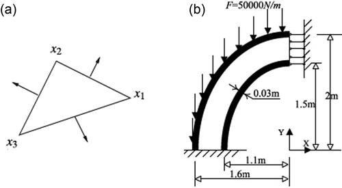
Let the boundary $\Gamma =\partial \Omega$ is discretized into $N_e$ surface triangles boundary elements ${\tau }_e$ as (Figure 2(a)) (68) $$\Gamma \approx {\Gamma }_h=\underset{e=1}{\overset{{\mathit{N}}_{\mathit{e}}}{\cup }}{\tau }_e.\mathrm{}$$(68)

Figure 2. (a) Triangular boundary element. (b) geometry of elliptical sandwich structure.

We can now describe the two subspaces on ${\Gamma }_h$ as (69) $$S_h\left[k\right]\left({\Gamma }_{N,\mathrm{}h}\right)≔\mathit{span}{\left\{{\phi }_i^{\alpha }\left[k\right]\right\}}_{i=1}^{\mathbb{i}},\mathrm{}\alpha \ge 1,\mathrm{}$$(69) (70) $$S_h\left[k\right]\left({\Gamma }_{D,\mathrm{}h}\right)≔\mathit{span}{\left\{{\psi }_j^{\beta }\left[k\right]\right\}}_{j=1}^{\mathbb{j}},\mathrm{}\beta \ge 0.\mathrm{}$$(70) where the unknown Neumann datum and unknown Dirichlet datum are approximated as (71) $${\widehat{u}}^g\left[k\right]\left(x\right)\approx {\widehat{u}}_h^g\left[k\right]\left(x\right)=\sum _{i=1}^{\mathbb{i}}{\widehat{u}}_{h,\mathrm{}i}^g\left[k\right]{\phi }_i^{\alpha }\left[k\right]\left(x\right)\in S_h\left[k\right]\left({\Gamma }_{N,\mathrm{}h}\right),\mathrm{}$$(71) (72) $${\widehat{t}}^g\left[k\right]\left(x\right)\approx {\widehat{t}}_h^g\left[k\right]\left(x\right)=\sum _{j=1}^{\mathbb{j}}{\widehat{t}}_{h,\mathrm{}j}^g\left[k\right]{\psi }_j^{\beta }\left[k\right]\left(x\right)\in S_h\left[k\right]\left({\Gamma }_{D,\mathrm{}h}\right).\mathrm{}$$(72) where ${\phi }_i^{\alpha }\left[k\right]$ are continuous polynomial shape functions, ${\psi }_j^{\beta }\left[k\right]$ are piecewise discontinuous polynomial shape functions and $k=1,\mathrm{}2,\mathrm{}3,\mathrm{}4$ are the poroelastic degrees of freedom.

Substituting (71(71) $${\widehat{u}}^g\left[k\right]\left(x\right)\approx {\widehat{u}}_h^g\left[k\right]\left(x\right)=\sum _{i=1}^{\mathbb{i}}{\widehat{u}}_{h,\mathrm{}i}^g\left[k\right]{\phi }_i^{\alpha }\left[k\right]\left(x\right)\in S_h\left[k\right]\left({\Gamma }_{N,\mathrm{}h}\right),\mathrm{}$$(71) ) and (72(72) $${\widehat{t}}^g\left[k\right]\left(x\right)\approx {\widehat{t}}_h^g\left[k\right]\left(x\right)=\sum _{j=1}^{\mathbb{j}}{\widehat{t}}_{h,\mathrm{}j}^g\left[k\right]{\psi }_j^{\beta }\left[k\right]\left(x\right)\in S_h\left[k\right]\left({\Gamma }_{D,\mathrm{}h}\right).\mathrm{}$$(72) ) into (67(67) $$C\left(x\right){\widehat{u}}^g\left({x,\mathrm{}s}_{\ell }\right)=\left(\widehat{v}{\widehat{t}}^g\right)\left({x,\mathrm{}s}_{\ell }\right)-\left({\widehat{k}\widehat{u}}^g\right)\left({x,\mathrm{}s}_{\ell }\right),\mathrm{}\ell =0\dots \dots .N.\mathrm{}$$(67) ), we obtain (73) $${\left[\genfrac{}{}{0pt}{}{{\widehat{V}}_{DD}\mathrm{}}{{\widehat{V}}_{ND}\mathrm{}}\genfrac{}{}{0pt}{}{-{\widehat{K}}_{DN}\mathrm{}}{-\left(C+{\widehat{K}}_{NN}\right)}\right]}_{\ell }{\left[\genfrac{}{}{0pt}{}{{\widehat{t}}_{D,h}^g}{{\widehat{u}}_{N,h}^g}\right]}_{\ell }={\left[\genfrac{}{}{0pt}{}{-{\widehat{V}}_{DN}}{{-\widehat{V}}_{NN}}\mathrm{}\genfrac{}{}{0pt}{}{\left(C+{\widehat{K}}_{DD}\right)}{{\widehat{K}}_{ND}\mathrm{}}\right]}_{\ell }{\left[\genfrac{}{}{0pt}{}{{\widehat{g}}_{N,\mathrm{}h}^g}{{\widehat{g}}_{D,\mathrm{}h}^g}\right]}_{\ell }\mathrm{}\ell =0\dots \mathrm{}N.\mathrm{}$$(73) where (74) $${\widehat{S}}_{NN}≔{\widehat{V}}_{ND}{\widehat{V}}_{DD}^{-1}{\widehat{K}}_{DN}-\left(C+{\widehat{K}}_{NN}\right).\mathrm{}$$(74)

According to Maier, Diligenti, and Carini (1991) and considering matrices instead of integral operators, we can write (73(73) $${\left[\genfrac{}{}{0pt}{}{{\widehat{V}}_{DD}\mathrm{}}{{\widehat{V}}_{ND}\mathrm{}}\genfrac{}{}{0pt}{}{-{\widehat{K}}_{DN}\mathrm{}}{-\left(C+{\widehat{K}}_{NN}\right)}\right]}_{\ell }{\left[\genfrac{}{}{0pt}{}{{\widehat{t}}_{D,h}^g}{{\widehat{u}}_{N,h}^g}\right]}_{\ell }={\left[\genfrac{}{}{0pt}{}{-{\widehat{V}}_{DN}}{{-\widehat{V}}_{NN}}\mathrm{}\genfrac{}{}{0pt}{}{\left(C+{\widehat{K}}_{DD}\right)}{{\widehat{K}}_{ND}\mathrm{}}\right]}_{\ell }{\left[\genfrac{}{}{0pt}{}{{\widehat{g}}_{N,\mathrm{}h}^g}{{\widehat{g}}_{D,\mathrm{}h}^g}\right]}_{\ell }\mathrm{}\ell =0\dots \mathrm{}N.\mathrm{}$$(73) ) in compact form as follows (75) $$Ly=\overline{f}\mathrm{}$$(75) where $$L=\left[\genfrac{}{}{0pt}{}{{\widehat{V}}_{DD}\mathrm{}}{{\widehat{V}}_{ND}\mathrm{}}\genfrac{}{}{0pt}{}{-{\widehat{K}}_{DN}\mathrm{}}{-\left(C+{\widehat{K}}_{NN}\right)}\right]$$ $$y=\left\{\begin{array}{c}{\widehat{u}}_h^g\left[k\right]\left(x\right)\\ {\widehat{t}}_h^g\left[k\right]\left(x\right)\end{array}\right.$$ $$\overline{f}={\left[\genfrac{}{}{0pt}{}{-{\widehat{V}}_{DN}}{{-\widehat{V}}_{NN}}\mathrm{}\genfrac{}{}{0pt}{}{\left(C+{\widehat{K}}_{DD}\right)}{{\widehat{K}}_{ND}\mathrm{}}\right]}_{\ell }{\left[\genfrac{}{}{0pt}{}{{\widehat{g}}_{N,\mathrm{}h}^g}{{\widehat{g}}_{D,\mathrm{}h}^g}\right]}_{\ell }\mathrm{}\ell =0\dots \mathrm{}N$$ $${\widehat{u}}_h^g\left[k\right]\left(x\right)=\sum _{i=1}^{\mathbb{i}}{\widehat{u}}_{h,\mathrm{}i}^g\left[k\right]{\phi }_i^{\alpha }\left[k\right]\left(x\right)\in S_h\left[k\right]\left({\Gamma }_{N,\mathrm{}h}\right)$$ $${\widehat{t}}_h^g\left[k\right]\left(x\right)=\sum _{j=1}^{\mathbb{j}}{\widehat{t}}_{h,\mathrm{}j}^g\left[k\right]{\psi }_j^{\beta }\left[k\right]\left(x\right)\in S_h\left[k\right]\left({\Gamma }_{D,\mathrm{}h}\right)$$

According to Maier, Diligenti, and Carini (1990) with consideration of $f=Ly$ and taking into account (61(61) $$\left(f\mathrm{\ast }g\right)\left(t_n\right)\approx \sum _{k=0}^n{\omega }_{n-k}^{\Delta t}\left(\widehat{f}\right)g\left(t_k\right).\mathrm{}$$(61) ), thus, it is easily to prove that (76) $$〈Ly,\mathrm{}y\mathrm{\prime }〉=〈L{y}^{\mathrm{\prime }},\mathrm{}y〉\text{for any y and y′}$$(76)

Due to the symmetry of $L$ in space and time, we can write the following variational formula (see Maier et al., 1990, 1991) (77) $$F\left(u^g\text{on}{\Gamma }_N,\mathrm{}{t}^g\text{on}{\Gamma }_D\right)=\frac{1}{2}〈Ly,\mathrm{}y〉-〈\overline{f},\mathrm{}y〉\mathrm{}$$(77)

where $\mathrm{x}$ is a field point, $\mathrm{\xi }$ is a load point and

Now, we evaluate the consequent variation of the functional (77(77) $$F\left(u^g\text{on}{\Gamma }_N,\mathrm{}{t}^g\text{on}{\Gamma }_D\right)=\frac{1}{2}〈Ly,\mathrm{}y〉-〈\overline{f},\mathrm{}y〉\mathrm{}$$(77) ) due to variation $\delta y$ of the variables (78) $$\delta F={\delta }^{\left(1\right)}F+{\delta }^{\left(2\right)}F\mathrm{}$$(78) (79) $${\delta }^{\left(1\right)}F=\frac{1}{2}〈Ly,\mathrm{}\delta y〉+\frac{1}{2}〈L\delta y,\mathrm{}y〉-〈\overline{f},\mathrm{}\delta y〉\mathrm{}$$(79) (80) $${\delta }^{\left(2\right)}F=\frac{1}{2}〈L\delta y,\mathrm{}\delta y〉\mathrm{}$$(80)

By using (75(75) $$Ly=\overline{f}\mathrm{}$$(75) ) and (76(76) $$〈Ly,\mathrm{}y\mathrm{\prime }〉=〈L{y}^{\mathrm{\prime }},\mathrm{}y〉\text{for any y and y′}$$(76) ), we can write for any $\delta y$ (81) $${\delta }^{\left(1\right)}F=〈Ly,\mathrm{}\delta y〉-〈\overline{f},\mathrm{}\delta y〉+〈Ly-\overline{f},\mathrm{}\delta y〉=0\mathrm{}$$(81)

Thus, $y$ is the boundary solution

5. Design sensitivity analysis and topology optimization

The considered optimization problem can be defined as follows (Matsumoto, Tanaka, & Ogawa, 2003) (82) $$\underset{\stackrel{̿}{\rho }\in {\mathbb{R}}^N}{\min }{f}_0\left(\stackrel{̿}{\rho },\mathrm{}u,\mathrm{}p\right),\mathrm{}$$(82) subject to (83) $$r\left(\stackrel{̿}{\rho },\mathrm{}u\left(\tau \right),\mathrm{}p\left(\tau \right),\mathrm{}\dot{u}\left(\tau \right),\mathrm{}\dot{p}\left(\tau \right)\right)=0,\mathrm{}$$(83) (84) $$\frac{1}{V_0}\mathrm{}\sum _{e=1}^N{\stackrel{̿}{\rho }}_e{\upsilon }_e-\stackrel{̿}{\gamma }\mathrm{}\le 0,\mathrm{}$$(84)

(85) $${\rho }_1\le {\stackrel{̿}{\rho }}_e\le {\rho }_2\mathrm{for}e=1,\mathrm{}N,$$(85)

where $r$ is the residual of state equation, $N$ is the design variables number, $\stackrel{̿}{\gamma }$ is a fraction of solid volume. Also, we assumed that $\left({\rho }_1,\mathrm{}{\rho }_2\right)=\left(0.01,\mathrm{}0.99\right).$

Eq. (67(67) $$C\left(x\right){\widehat{u}}^g\left({x,\mathrm{}s}_{\ell }\right)=\left(\widehat{v}{\widehat{t}}^g\right)\left({x,\mathrm{}s}_{\ell }\right)-\left({\widehat{k}\widehat{u}}^g\right)\left({x,\mathrm{}s}_{\ell }\right),\mathrm{}\ell =0\dots \dots .N.\mathrm{}$$(67) ) can be written as (86) $$\mathcal{F}=\mathbb{A}\mathbb{Q}-\mathbb{B}\mathbb{V}.\mathrm{}$$(86)

The objective function may be defined as (87) $$\mathcal{G}={\int }_0^T\mathit{\hslash }(\mathbb{Q},\mathrm{}\mathbb{V},\mathrm{}\stackrel{̿}{\rho },\mathrm{}\tau )d\tau .\mathrm{}$$(87)

The augmented objective function can be described as (Igumnov & Markov, 2016; Schanz, 2001) (88) $$L={\int }_0^T\mathit{\hslash }(\mathbb{Q},\mathrm{}\mathbb{V},\mathrm{}\stackrel{̿}{\rho },\mathrm{}\tau )d\tau +{\int }_0^T{\lambda }^T\left(\mathbb{A}\mathbb{Q}-\mathbb{B}\mathrm{}\mathbb{V}-\mathcal{F}\right)d\tau .\mathrm{}$$(88)

where $\mathbb{A}$ and $\mathbb{B}$ are nonsymmetric matrices and $\lambda$ is the adjoint variable vector $$\frac{dL}{d\stackrel{̿}{\rho }}={\int }_0^T\frac{d\mathit{\hslash }}{d\stackrel{̿}{\rho }}d\tau +{\int }_0^T{\lambda }^T\left(\frac{\partial \mathbb{A}}{\partial \stackrel{̿}{\rho }}\mathbb{Q}-\frac{\partial \mathbb{B}}{\partial \stackrel{̿}{\rho }}\mathbb{V}-\frac{\partial \mathcal{F}}{\partial \stackrel{̿}{\rho }}\right)d\tau +{\int }_0^T\left(\frac{\partial \mathit{\hslash }}{\partial \mathbb{Q}}\frac{d\mathbb{Q}}{d\stackrel{̿}{\rho }}+\frac{\partial \mathit{\hslash }}{\partial \mathbb{V}}\frac{d\mathbb{V}}{d\stackrel{̿}{\rho }}\right)d\tau$$ (89) $$+{\int }_0^T{\lambda }^T\left(\mathbb{A}\frac{d\mathbb{V}}{d\stackrel{̿}{\rho }}+\mathbb{B}\frac{d\mathbb{Q}}{d\stackrel{̿}{\rho }}\right)d\tau .\mathrm{}$$(89)

According to Schanz (2001), the sensitivities can be calculated as (90) $$\frac{dL}{d\stackrel{̿}{\rho }}={\int }_0^T\frac{d\mathit{\hslash }}{d\stackrel{̿}{\rho }}d\tau +{\int }_0^T{\lambda }^T\left(\frac{\partial \mathbb{A}}{\partial \stackrel{̿}{\rho }}\mathbb{Q}-\frac{\partial \mathbb{B}}{\partial \stackrel{̿}{\rho }}\mathbb{V}-\frac{\partial \mathcal{F}}{\partial \stackrel{̿}{\rho }}\right)d\tau .\mathrm{}$$(90)

By implementing the Moving Asymptotes Method (MAM) with the adjoint variable method (Itzá, Viveros, & Parra, 2016) a standard filter densities ${\overline{\mathrm{\rho }}}_{\mathrm{e}}\mathrm{}$ and the sensitivities for the BEM analysis can be computed as follows (Bourdin, 2001; Bruns & Tortorelli, 2001) (91) $${\overline{\rho }}_e=\frac{\sum _{i\in N_e}^{}\mathcal{w}\left({\mathcal{x}}_i,\mathrm{}{\mathcal{x}}_e\right){\upsilon }_i{\rho }_i}{\sum _{i\in N_e}^{}\mathcal{w}\left({\mathcal{x}}_i,\mathrm{}{\mathcal{x}}_e\right){\upsilon }_i},\mathcal{}\mathcal{w}\left({\mathcal{x}}_i,\mathrm{}{\mathcal{x}}_e\right)=R-‖{\mathcal{x}}_i-{\mathcal{x}}_e‖.\mathrm{}$$(91) (92) $$\frac{d\mathrm{}{f}_0}{d\mathrm{}{\stackrel{̿}{\rho }}_e}=\sum _{i\in N_e}^{}\frac{d\mathrm{}{f}_0}{d\mathrm{}{\overline{\rho }}_i}\frac{\mathcal{w}\left({\mathcal{x}}_e,\mathrm{}{\mathcal{x}}_i\right){\upsilon }_e}{\sum _{j\in N_i}^{}\mathcal{w}\left({\mathcal{x}}_j,\mathrm{}{\mathcal{x}}_i\right){\upsilon }_j}.\mathrm{}$$(92)

Where $\mathcal{w}$ is the weighting function, ${\mathcal{x}}_{\mathrm{e}}$ are the element coordinates, ${\mathrm{N}}_{\mathrm{e}}$ denotes the elements set whose distance from $\mathrm{e}$ is lower than $R$ and ${\upsilon }_i$ is the volume of element.

6. Numerical results and discussion

The proposed technique in the current work should be applicable to any anisotropic thermo-poroelastic problem. The models of Braun, Ghabezloo, Delage, Sulem, and Conil (2018) and Giot, Granet, Faivre, Massoussi, and Huang (2018) may be considered as special cases of our current complex and general study. To illustrate the numerical results calculated by the proposed technique presented in the current paper, the material considered as an anisotropic poroelastic material is a prismatic solid, and the physical parameters for this material are (Braun et al., 2018):

The elasticity tensor of anisotropic prismatic structure (93) $$C_{\mathit{ablg}}=\left(\begin{array}{ccc}\begin{array}{c}\begin{array}{cc}60.23& 18.67\end{array}\\ \begin{array}{cc}18.67& 21.26\end{array}\end{array}& \begin{array}{c}\begin{array}{cc}18.96& -7.69\end{array}\\ \begin{array}{cc}9.36& -3.74\end{array}\end{array}& \begin{array}{c}\begin{array}{cc}15.60& -25.28\end{array}\\ \begin{array}{cc}4.21& -8.47\end{array}\end{array}\\ \begin{array}{c}\begin{array}{cc}18.96& 9.36\end{array}\\ \begin{array}{cc}-7.69& -3.74\end{array}\end{array}& \begin{array}{c}\begin{array}{cc}47.04& -8.82\end{array}\\ \begin{array}{cc}-8.82& 10.1\end{array}8\end{array}& \begin{array}{c}\begin{array}{cc}15.28& -8.31\end{array}\\ \begin{array}{cc}-9.54& 5.69\end{array}\end{array}\\ \begin{array}{c}\begin{array}{cc}15.60& 4.21\end{array}\\ \begin{array}{cc}-25.28& -8.47\end{array}\end{array}& \begin{array}{c}\begin{array}{cc}15.28& -9.54\end{array}\\ \begin{array}{cc}-8.31& 5.69\end{array}\end{array}& \begin{array}{c}\begin{array}{cc}21.19& -8.54\end{array}\\ \begin{array}{cc}-8.54& 20.75\end{array}\end{array}\end{array}\right).\mathrm{}$$(93) where $\varphi =0.15,$ $k=0.987\times {10}^{-15}{m}^2,$ ${\rho }_s=1600kg/m^3,$ ${\rho }_{\mathcal{F}}=1113\mathrm{}kg/m^3,\mathrm{}p=25\mathrm{}\mathit{MPa},$ $\mathrm{}Q/R=0.65,$ $\mathbb{C}=0.66,$ $\mu =0.001,$ and $\Delta t=0.0007\mathrm{}s.$

The conditions have been considered in the calculations are as follows $$\text{at}\tau =0\mathrm{}{u}_1=u_2=u_3=v_1=v_2=v_3=p=0,$$ (94) $$\frac{\partial u_1}{\partial \tau }=\frac{\partial u_2}{\partial \tau }=\frac{\partial u_3}{\partial \tau }=\frac{\partial v_1}{\partial \tau }=\frac{\partial v_2}{\partial \tau }=\frac{\partial v_3}{\partial \tau }=\frac{\partial p}{\partial \tau }=0,\mathrm{}$$(94) (95) $$\text{at}{x}_1=0\mathrm{}{u}_1=u_2=u_3=v_1=v_2=v_3=0,\mathrm{}p=0\mathrm{}\forall \mathrm{}\tau \ge 0,\mathrm{}$$(95) (96) $$\text{at}{x}_1=\underset{¯}{\gamma }\mathrm{}{u}_1=u_2=u_3=v_1=v_2=v_3=0,\mathrm{}p=0\mathrm{}\forall \mathrm{}\tau \ge 0,\mathrm{}$$(96) (97) $$\text{at}{x}_2=0\mathrm{}{u}_1=u_2=u_3=v_1=v_2=v_3=0,\mathrm{}p=0\mathrm{}\forall \mathrm{}\tau \ge 0,\mathrm{}$$(97) (98) $$\text{at}{x}_2=\underset{¯}{\beta }\mathrm{}{u}_1=u_2=u_3=v_1=v_2=v_3=0,\mathrm{}p=0\mathrm{}\forall \mathrm{}\tau \ge 0,\mathrm{}$$(98) (99) $$\text{at}{x}_3=0\mathrm{}{u}_1=u_2=u_3=v_1=v_2=v_3=0,\mathrm{}p=0\mathrm{}\forall \mathrm{}\tau \ge 0,\mathrm{}$$(99) (100) $$\text{at}{x}_3=\underset{¯}{\alpha }\mathrm{}{u}_1=u_2=u_3=v_1=v_2=v_3=0,\mathrm{}p=0\mathrm{}\forall \mathrm{}\tau \ge 0.\mathrm{}$$(100)

Figure 2(b) shows the considered structure geometry. Table 1 shows the structure optimal design using CVBEM considered in this paper. Table 2 clears the comparison of computer resources needed for FEM and CVBEM for numerical simulation of elliptical sandwich structure. Thermo-poroelastic stresses ${\sigma }_{11},$ ${\sigma }_{12},$ ${\sigma }_{22},$ ${\sigma }_{13},$ ${\sigma }_{23},$ ${\sigma }_{33}$ sensitivities variations with the time are plotted in Figures 3–8, and we can see that the anisotropy has a signicant effect on the Thermo-poroelastic stresses sensitivities. Also, the results are highly sensitive to assumed initial conditions. The displacement and pore pressure variations with the time are plotted in Figures 9 and 10 for the analytical, FEM and CVBEM methods to demonstrate the validity of our implemented technique. It is noticed from these figures that the results of the CVBEM are in very excellent agreement with those obtained using the analytical method of Braun et al. (2018) and FEM of Giot et al. (2018). Our results thus confirm that our technique is efficient and precise.

Figure 3. Variation of the ${\sigma }_{11}$ sensitivity with time $t.$

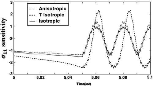
Figure 4. Variation of the ${\sigma }_{12}$ sensitivity with time $t.$

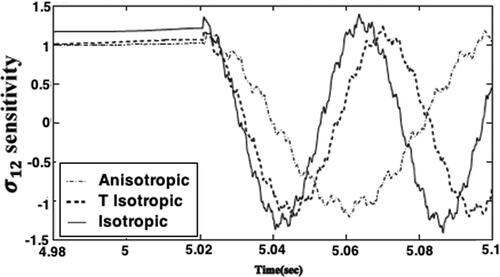
Figure 5. Variation of the ${\sigma }_{22}$ sensitivity with time $t.$

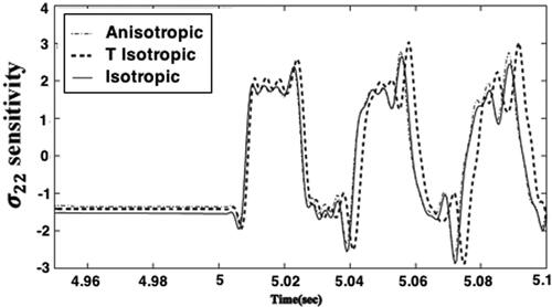
Figure 6. Variation of the ${\sigma }_{13}$ sensitivity with time $t.$

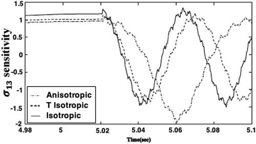
Figure 7. Variation of the ${\sigma }_{23}$ sensitivity with time $t.$

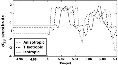
Figure 8. Variation of the ${\sigma }_{33}$ sensitivity with time $t.$

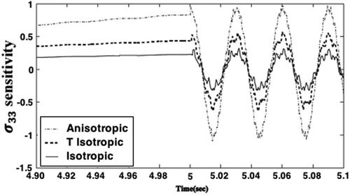
Figure 9. Variation of the displacement $u$ with time $t.$

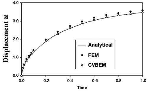
Figure 10. Variation of the pore pressure $p$ with time $t.$

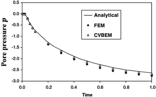
Table 1. Investigation of the influence of anisotropy in an elliptical sandwich structure.

Initial design			Optimum design
Isotropic	T-Isotropic	Anisotropic	Isotropic	T-Isotropic	Anisotropic

Table. 2. Comparison of computer resources needed for FEM and CVBEM modelling of elliptical sandwich structure.

	FEM	CVBEM
Number of nodes	28000	28
Number of elements	9850	28
CPU-Time (min.)	140	2
Memory (MByte)	90	0.5
Disc space (MByte)	180	0
Accuracy of results (%)	2.5	1.5

7. Conclusion

The CVBEM technique is proposed for transient studies of thermo-poroelastic optimization problems, where the regularization can be performed using integration by parts to remove the strong singularity and improve the efficiency of our proposed method. The CVBEM is very useful for problems where time-domain fundamental solutions are not known, because it utilizes the Laplace-domain fundamental solutions of the governing equations of the problem. Also, our proposed technique reduces the computational time and memory. For these mentioned reasons, our proposed CVBEM is very effective, accurate and powerful technique. The accuracy, efficiency and validity of our proposed CVBEM technique were confirmed by comparing the obtained results of our considered problem with the corresponding analytical results of Braun et al. (2018) and with the FEM results of Giot et al. (2018), it can be noticed that the CVBEM results show excellent agreement with the analytical and numerical FEM results, our results thus confirm that the proposed CVBEM technique is very effective, accurate and powerful technique for anisotropic thermo-poroelastic optimization problems. Understanding the design sensitivity and optimization of anisotropic thermo-poroelastic structures are very important in many fields such as geothermal engineering, petroleum engineering, geomechanics engineering, geotechnical engineering, biomechanics engineering, material science and material engineering etc.

Disclosure statement

No potential conflict of interest was reported by the author.

References

- Abd-Alla, A. M., El-Naggar, A. M., & Fahmy, M. A. (2003). Magneto-thermoelastic problem in non-homogeneous isotropic cylinder. Heat and Mass Transfer, 39(7), 625–629. doi:10.1007/s00231-002-0370-3
- Abd-Alla, A. M., Fahmy, M. A., & El-Shahat, T. M. (2008). Magneto-thermo-elastic problem of a rotating non-homogeneous anisotropic solid cylinder. Archive of Applied Mechanics, 78(2), 135–148. Issue doi:10.1007/s00419-007-0147-8
- Bendsoe, M. P., & Sigmund, O. (2004). Topology optimization: Theory, methods, and applications. Berlin, Heidelberg: Springer-Verlag.
- Biot, M. A. (1956a). Theory of propagation of elastic waves in a fluid- saturated porous solid. I. Low frequency range. The Journal of the Acoustical Society of America, 28(2), 168–178. doi:10.1121/1.1908239
- Biot, M. A. (1956b). Theory of propagation of elastic waves in a fluid- saturated porous solid. II. Higher frequency range. The Journal of the Acoustical Society of America, 28(2), 179–191. doi:10.1121/1.1908241
- Bonnet, G. (1987). Basic singular solutions for a poroelastic medium in the dynamic range. The Journal of the Acoustical Society of America, 82(5), 1758–1763. doi:10.1121/1.395169
- Bonnet, G., & Auriault, J. L. (1985). Dynamics of saturated and deform- able porous media: Homogenization theory and determination of the solid-liquid coupling coefficients. Physics of finely divided matter, Berlin: Springer Verlag, pp 306–316. doi:10.1007/978-3-642-93301-1_37
- Bourdin, B. (2001). Filters in topology optimization. International Journal for Numerical Methods in Engineering, 50(9), 2143–2158. doi:10.1002/nme.116
- Bourdin, B., & Chambolle, A. (2003). Design-dependent loads in topology optimization, ESAIM: Control. Esaim: Control, Optimisation and Calculus of Variations, 9, 19–48. doi:10.1051/cocv:2002070
- Braun, P., Ghabezloo, S., Delage, P., Sulem, J., & Conil, N. (2018). Theoretical Analysis of Pore Pressure Diffusion in Some Basic Rock Mechanics Experiments. Rock Mechanics and Rock Engineering, 51 (5), 1361–1378. doi:10.1007/s00603-018-1410-8
- Bruns, T., & Tortorelli, D. (2001). Topology optimization of non-linear elastic structures and compliant mechanisms. Computer Methods in Applied Mechanics and Engineering, 190 (26-27), 3443–3459. doi:10.1016/S0045-7825(00)00278-4
- Deaton, J. D., & Grandhi, R. V. (2014). A survey of structural and multidisciplinary continuum topology optimization: Post 2000. Structural and Multidisciplinary Optimization, 49(1), 1–38. doi:10.1007/s00158-013-0956-z
- Domínguez, J. (1993). Boundary Elements in Dynamics, Southampton: Computational Mechanics Publication.
- El-Naggar, A. M., Abd-Alla, A. M., & Fahmy, M. A. (2003). The propagation of thermal stresses in an infinite elastic slab. Applied Mathematics and Computation, 12, 220–226. doi:10.1016/j.amc.2003.08.116
- Fahmy, M. A. (2008). Thermoelastic stresses in a rotating non- homogeneous anisotropic body. Numerical Heat Transfer, Part A: Applications, 53(9), 1001–1011. doi:10.1080/10407780701789179
- Fahmy, M. A. (2011). A time-stepping DRBEM for magneto-thermo-viscoelastic interactions in a rotating nonhomogeneous anisotropic solid. International Journal of Applied Mechanics, 3(4), 711–734. doi:10.1142/S1758825111001202
- Fahmy, M. A. (2012a). A time-stepping DRBEM for the transient magneto-thermo-visco-elastic stresses in a rotating non-homogeneous anisotropic solid. Engineering Analysis with Boundary Elements, 36(3), 335–345. doi:10.1016/j.enganabound.2011.09.004
- Fahmy, M. A. (2012b). Transient magneto-thermoviscoelastic plane waves in a non-homogeneous anisotropic thick strip subjected to a moving heat source. Applied Mathematical Modelling, 36(10), 4565–4578. doi:10.1016/j.apm.2011.11.036
- Fahmy, M. A. (2012c). The effect of rotation and inhomogeneity on the transient magneto-thermoviscoelastic stresses in an anisotropic solid, ASME. Journal of Applied Mechanics, 79(5), 051015. doi:10.1115/1.4006258
- Fahmy, M. A. (2012d). Transient magneto-thermo-viscoelastic stresses in a rotating nonhomogeneous anisotropic solid with and without a moving heat source. Journal of Engineering Physics and Thermophysics, 85(4), 950–958. doi:10.1007/s10891-012-0735-5
- Fahmy, M. A. (2012e). Transient magneto-thermo-elastic stresses in an anisotropic viscoelastic solid with and without a moving heat source. Numerical Heat Transfer, Part A: Applications, 61(8), 633–650. doi:10.1080/10407782.2012.667322
- Fahmy, M. A. (2013a). Generalized magneto-thermo-viscoelastic problems of rotating functionally graded anisotropic plates by the dual reciprocity boundary element method. Journal of Thermal Stresses, 36(3), 284–220. doi:10.1080/01495739.2013.765206
- Fahmy, M. A. (2013b). Implicit-Explicit time integration DRBEM for generalized magneto-thermoelasticity problems of rotating anisotropic viscoelastic functionally graded solids. Engineering Analysis with Boundary Elements, 37(1), 107–115. doi:10.1016/j.enganabound.2012.08.002
- Fahmy, M. A. (2013c). A three-dimensional generalized magneto-thermo-viscoelastic problem of a rotating functionally graded anisotropic solids with and without energy dissipation. Numerical Heat Transfer, Part A: Applications, 63(9), 713–733. doi:10.1080/10407782.2013.751317
- Fahmy, M. A. (2017a). Computerized boundary element solutions for thermoelastic problems: Applications to functionally graded anisotropic structures. Saarbrücken, Germany: LAP Lambert Academic Publishing.
- Fahmy, M. A. (2017b). Boundary element computation of shape sensitivity and optimization: Applications to functionally graded anisotropic structures. Saarbrücken, Germany: LAP Lambert Academic Publishing.
- Fahmy, M. A. (2018a). Shape design sensitivity and optimization for two-temperature generalized magneto-thermoelastic problems using time-domain DRBEM. Journal of Thermal Stresses, 41(1), 119–138. doi:10.1080/01495739.2017.1387880
- Fahmy, M. A. (2018b). Shape design sensitivity and optimization of anisotropic functionally graded smart structures using bicubic B-splines DRBEM. Engineering Analysis with Boundary Elements, 87, 27–35. doi:10.1016/j.enganabound.2017.11.005
- Fahmy, M. A. (2018c). Boundary element algorithm for modeling and simulation of dual phase lag bioheat transfer and biomechanics of anisotropic soft tissues. International Journal of Applied Mechanics, 10(10), 1850108. doi:10.1142/S1758825118501089
- Fahmy, M. A. (2019a). Modeling and optimization of anisotropic viscoelastic porous structures using CQBEM and moving asymptotes algorithm. Arabian Journal for Science and Engineering, 44(2), 1671–1684. doi:10.1007/s13369-018-3652-x
- Fahmy, M. A. (2019b). A new LRBFCM-GBEM modeling algorithm for general solution of time fractional order dual phase lag bioheat transfer problems in functionally graded tissues. Numerical Heat Transfer, Part A: Applications, 75(9), 616–626. doi:10.1080/10407782.2019.1608770
- Fahmy, M. A. (2019c). Boundary element modeling and simulation of biothermomechanical behavior in anisotropic laser-induced tissue hyperthermia. Engineering Analysis with Boundary Elements, 101, 156–164. doi:10.1016/j.enganabound.2019.01.006
- Fahmy, M. A. (2019d). Design optimization for a simulation of rotating anisotropic viscoelastic porous structures using time-domain OQBEM. Mathematics and Computers in Simulation, 166, 193–205. doi:10.1016/j.matcom.2019.05.004
- Fahmy, M. A. (2019e). A new boundary element strategy for modeling and simulation of three temperatures nonlinear generalized micropolar-magneto-thermoelastic wave propagation problems in FGA structures. Engineering Analysis with Boundary Elements, 108, 192–200. doi:10.1016/j.enganabound.2019.08.006
- Fahmy, M. A., & El-Shahat, T. M. (2008). The effect of initial stress and inhomogeneity on the thermoelastic stresses in a rotating anisotropic solid. Archive of Applied Mechanics, 78(6), 431–442. doi:10.1007/s00419-007-0150-0
- Giles, M. B., & Pierce, N. A. (2000). An introduction to the adjoint approach to design. Flow, Turbulence and Combustion, 65(3/4), 393–415. doi:10.1023/A:1011430410075
- Giot, R., Granet, S., Faivre, M., Massoussi, N., & Huang, J. (2018). A transversely isotropic thermo-poroelastic model for claystone: Parameter identification and application to a 3D underground structure. Geomechanics and Geoengineering, 13 (4), 246–263. doi:10.1080/17486025.2018.1445874
- Gunzburger, M. D. (2003). Perspectives in flow control and optimization. USA:SIAM. doi:10.1137/1.9780898718720
- Hinze, M., Pinnau, R., Ulbrich, M., & Ulbrich, S. (2009). Optimization with PDE constraints (Vol. 23). Netherlands, Dordrecht: Springer. doi:10.1007/978-1-4020-8839-1
- Igumnov, L. A., & Markov, I. P. (2016). Boundary-element modeling of three-dimensional anisotropic viscoelastic solids. In I. A. Parinov, S. H. Chang, & V. Y. Topolov (Eds.), Advanced materials: Manufacturing, physics, mechanics and applications (pp. 517–526). Switzerland: Springer International Publishing. doi:10.1007/978-3-319-26324-3_36
- Iqbal, M. A., Mohyud-Din, S. T., & Bin-Mohsin, B. (2016). A study of nonlinear biochemical reaction model. International Journal of Biomathematics, 9(5), 1650071. doi:10.1142/S1793524516500716
- Itzá, R., Viveros, U. I., & Parra, J. O. (2016). Optimal implicit 2-D finite differences to model wave propagation in poroelastic media. Geophysical Journal International, 206(2), 1111–1125. doi:10.1093/gji/ggw180
- Khan, U., Ellahi, R., Khan, R., & Mohyud-Din, S. T. (2017). Extracting new solitary wave solutions of benny-luke equation and phi-4 equation of fractional order by using (G'/G)-expansion method. Optical and Quantum Electronics, 49(11), 362. doi:10.1007/s11082-017-1191-4
- Kielhorn, L. (2009). A time-domain symmetric Galerkin BEM for viscoelastodynamics. In G. Brenn, G.A. Holzapfel, M. Schanz, & O. Steinbach (Eds.), Computation in engineering and science (Vol. 5), Austria: Graz University of Technology, Institute of Applied Mechanics.
- Koga, A. A., Lopes, E. C. C., Nova, H. F. V., de Lima, C. R., & Silva, E. C. N. (2013). Development of heat sink device by using topology optimization. International Journal of Heat and Mass Transfer, 64, 759–772. doi:10.1016/j.ijheatmasstransfer.2013.05.007
- Kontoleontos, E. A., Papoutsis-Kiachagias, E. M., Zymaris, A. S., Papadimitriou, D. I., & Giannakoglou, K. C. (2013). Adjoint-based constrained topology optimization for viscous flows, including heat transfer. Engineering Optimization, 45(8), 941–961. doi:10.1080/0305215X.2012.717074
- Lubich, C. (1988a). Convolution quadrature and discretized operational calculus. I. Numerische Mathematik, 52(2), 129–145. doi:10.1007/BF01398686
- Lubich, C. (1988b). Convolution quadrature and discretized operational calculus II. Numerische Mathematik, 52(4), 413–425. doi:10.1007/BF01462237
- Maier, G., Diligenti, M., & Carini, A. (1990). A Variational Formulation of the Boundary Element Method in Elastodynamics. In B. S. Annigeri & K. Tseng (Eds), Boundary element methods in engineering (pp. 268-275). Berlin, Heidelberg: Springer. doi:10.1007/978-3-642-84238-2_33
- Maier, G., Diligenti, M., & Carini, A. (1991). A variational approach to boundary element elastodynamic analysis and extension to multidomain problems. Computer Methods in Applied Mechanics and Engineering, 92(2), 193–213. doi:10.1016/0045-7825(91)90239-3
- Marck, G., Nemer, M., & Harion, J. L. (2013). Topology optimization of heat and mass transfer problems: Laminar flow. Numerical Heat Transfer Part B: Fundamentals, 63(6), 508–539. doi:10.1080/10407790.2013.772001
- Martins, J. R. R. A., & Hwang, J. T. (2013). Review and unification of methods for computing derivatives of multidisciplinary computational models. AIAA Journal, 51(11), 2582–2599. doi:10.2514/1.J052184
- Matsumori, T., Kondoh, T., Kawamoto, A., & Nomura, T. (2013). Topology optimization for fluid thermal interaction problems under constant input power. Structural and Multidisciplinary Optimization, 47(4), 571–581. doi:10.1007/s00158-013-0887-8
- Matsumoto, T., Tanaka, M., & Ogawa, Y. (2003). A simple technique for efficient evaluations of boundary integrals of time-harmonic elastodynamic BEM analyses for anisotropic solids. In K. J. Bathe (Ed.), Proceedings Second MIT Conference on Computational Fluid and Solid Mechanics (pp. 2071–2073). Oxford: Elsevier. doi:10.1016/B978-008044046-0.50508-X
- Messner, M., & Schanz, M. (2011). A regularized collocation boundary element method for linear poroelasticity. Computational Mechanics, 47(6), 669–680. doi:10.1007/s00466-010-0569-y
- Mohamed, N. A. (2019). Solving one- and two-dimensional unsteady Burgers' equation using fully implicit finite difference schemes. Arab Journal of Basic and Applied Sciences, 26(1), 254–268. doi:10.1080/25765299.2019.1613746
- Mohyud-Din, S. T., Irshad, A., Ahmed, N., & Khan, U. (2017). Exact solutions of (3 + 1)-dimensional generalized KP Equation Arising in Physics. Results in Physics, 7, 3901–3909. doi:10.1016/j.rinp.2017.10.007
- Mohyud-Din, S. T., Noor, M. A., & Noor, K. I. (2009). Traveling wave solutions of seventh-order generalized KdV equations using He's polynomials. International Journal of Nonlinear Sciences and Numerical Simulation, 10(2), 223–229. doi:10.1142/S0217979209052467
- Mohyud‐Din, S. T., Yıldırım, A., & Sarıaydın, S. (2011). Numerical soliton solution of the Kaup-Kupershmidt equation. International Journal of Numerical Methods for Heat & Fluid Flow, 21, 272–281. doi:10.1108/09615531111108459
- Nadarajah, S., & Jameson, A. (2000). A comparison of the continuous and discrete adjoint approach to automatic aerodynamic optimization. Proceeding of 38th Aerospace Sciences Meeting and Exhibit (pp. AIAA-2000-0667).
- Qian, X., & Dede, E. M. (2016). Topology optimization of a coupled thermal-fluid system under a tangential thermal gradient constraint. Structural and Multidisciplinary Optimization, 54(3), 531–551. doi:10.1007/s00158-016-1421-6
- Schanz, M. (2001). Wave propagation in viscoelastic and poroelastic continua: A boundary element approach, Part of the Lecture Notes in Applied Mechanics book series (LNACM, volume 2), Berlin: Springer-Verlag. doi: 10.1007/978-3-540-44575-3
- Shakeel, M., & Mohyud-Din, S. T. (2015). New (G′/G)-expansion method and its application to the Zakharov-Kuznetsov–Benjamin-Bona-Mahony (ZK–BBM) equation. Journal of the Association of Arab Universities for Basic and Applied Sciences, 18(1), 66–81. doi:10.1016/j.jaubas.2014.02.007
- Sikander, W., Khan, U., Ahmed, N., & Mohyud-Din, S. T. (2017). Optimal solutions for homogeneous and non-homogeneous equations arising in physics. Results in Physics, 7, 216–224. doi:10.1016/j.rinp.2016.12.018
- Sikander, W., Khan, U., & Mohyud-Din, S. T. (2017). Optimal solutions for the evolution of a social obesity epidemic model. The European Physical Journal Plus, 132(6), 257. doi:10.1016/j.rinp.2016.12.018
- Steinbach, O. (2008). Numerical approximation methods for elliptic boundary value problems. New York, NY: Springer. doi:10.1007/978-0-387-68805-3
- Sun, H. Q., & Chen, A. H. (2018). Exact solutions of the classical Boussinesq system. Arab Journal of Basic and Applied Sciences, 25(2), 85–91. doi:10.1080/25765299.2018.1449416
- Suresh, K. (2013). Efficient generation of large-scale pareto-optimal topologies. Structural and Multidisciplinary Optimization, 47(1), 49–61. doi:10.1007/s00158-012-0807-3
- Wang, C. Y., & Achenbach, J. D. (1994). Elastodynamic fundamental solution for anisotropic solids. Geophysical Journal International, 118(2), 384–392. doi:10.1111/j.1365-246X.1994.tb03970.x
- Wang, C. Y., & Achenbach, J. D. (1995). Three-dimensional time-harmonic elastodynamic Green’s functions for anisotropic solids. Proceedings of the Royal Society A: Mathematical, Physical and Engineering Sciences, 449(1937), 441–458. doi:10.1098/rspa.1995.0052
- Wang, M. Y., Wang, X., & Guo, D. (2003). A level set method for structural topology optimization. Computer Methods in Applied Mechanics and Engineering, 192(1-2), 227–246. doi:10.1016/S0045-7825(02)00559-5
- Xie, Y. M., & Steven, G. P. (1993). A simple evolutionary procedure for structural optimization. Computers & Structures, 49, 885–896. doi:10.1016/0045-7949(93)90035-C
- Yaji, K., Yamada, T., Kubo, S., Izui, K., & Nishiwaki, S. (2015). A topology optimization method for a coupled thermal–fluid problem using level set boundary expressions. International Journal of Heat and Mass Transfer, 81, 878–888. doi:10.1016/j.ijheatmasstransfer.2014.11.005
- Zhou, M., & Rozvany, G. I. N. (1991). The COC algorithm, Part II: Topological, geometrical and generalized shape optimization. Computer Methods in Applied Mechanics and Engineering, 89(1–3), 309–336. doi:10.1016/0045-7825(91)90046-9