An advanced dice similarity measure of generalized fuzzy numbers and its application in multicriteria decision making

Abstract

Multicriteria decision making (MCDM) is an important process to select best alternative among a set of alternatives based on preassigned multiple criteria. Presence of uncertainty due to lack of information/data, imprecision, vagueness etc. classical MCDM process becomes more complex and inappropriate. To overcome such types of situations, different types of fuzzy sets are explored and consequently fuzzy multicriteria decision making (FMCDM) was developed. In FMCDM problems, similarity measure of generalized fuzzy numbers plays crucial role in making appropriate decision by choosing best alternative. A handful number of work done on similarity measures are confronted in literature. Even though some advantages of these existing works are encountered, most of the works have impediments. In this regard, an attempt has been made to devise a similarity measure (SM) of GFNs with same or unequal height. It is observed that the proposed SM has the capability to overcome the deficiencies of the available earlier approaches and outplays in all the environments. To showcase the novelty and efficiency of the present SM comparative studies have been performed. Moreover, FMCDM problem has been solved under this setting and found that results obtained by this approach confronts human intuitions and analytical output.

Keywords:

• Generalized Fuzzy number
• multicriteria decision making
• similarity measure
• uncertainty/imprecision

1. Introduction

Uncertainty is intrinsic in any real word problems including decision making. Often uncertainty is disregarded for evading complication, and consequently solutions obtained in this process are rather a long way from the realism that directs to above or beneath inference. Therefore, it is most essential to incorporate uncertainty in that progression in order to overcome and resolve the deficiencies took place in the decision making process. Generally two types of uncertainties are taken into consideration viz., aleatory and epistemic uncertainty. Aleatory uncertainty in decision making arises due to randomness, intrinsic variability, stochasticity, variation through time or across space etc. Sometimes, it is simply called variability and the classical demonstration of variability is the probability distribution function. On the other hand, epistemic uncertainty occurs because of deficient of information or knowledge about the environment, measurement uncertainty, vagueness, small sample size, imprecision etc (Dutta & Hazarika, 2017). It should be noted that epistemic uncertainty can be abridged by further study while aleatory uncertainty can’t be abridged. Classical probability theory (PT) is generally explored to deal with aleatory uncertainty. Nevertheless, PT is not pertinent to handle epistemic uncertainty. Zadeh (1965) initiated the fuzzy set theory (FST) to surmount the inadequacies of PT and to deal with epistemic uncertainty as well. Afterward FST was effectively applied in diverse areas by different researchers. MCDM is a process to evaluate beast alternative or preference ordering of alternatives based on preset criteria via either a single person expert or a panel of experts, in which appropriateness of alternatives versus criteria, and the importance weights of criteria can be appraised using linguistic variables (Chen & Hwang, 1992). A linguistic variable is a variable whose values are words or sentences in a natural or artificial language (Zadeh, 1975). More often, linguistic variable or expressions are vague or uncertain (epistemic type) in nature and consequently they are represented by fuzzy numbers. Decision making under such environment is a crucial issue and similarity measures (SMs) of GFNs can be applied to perform decision making under such situations. Some recent approaches of SMs are encountered in literature such as similarity measures based on geometric distance was developed in Chen (1996) to assess mental work load and risk analysis, similarity measure was also proposed in Wei and Chen (2009) for fuzzy risk assessment; graded mean integration based similarity were presented in Hsieh (1999) and Lee (2002) for group decision making; center of gravity (COG) based similarity can be encountered in Chen and Chen (2001), similarity based on radius of gyration(ROG) was observed in Yong, Wenkang, Feng, and Qi (2004) for pattern recognition; both COG and geometric distance based similarity measure was proposed in Xu, Shang, Qian, and Shu (2010) for trapezoidal fuzzy numbers; again, geometric distance, perimeter, area and height based similarity measure was observed in Hejazi, Doostparast, and Hosseini (2011) for generalized fuzzy numbers; a cosine SM studied in Ye (2011) was expected interval based similarity measure was presented in Ye (2012) for group decision making; similarity measure via area and geometric distance was developed in Patra and Mondal (2015) for generalized trapezoidal fuzzy numbers; geometric distance, COG and perimeters based similarity was put forwarded in Khorshidi and Nikfalazar (2017) and applied in risk analysis; geometric distance, based on ROG and heights (Chutia & Gogoi, 2018) presented a similarity measure, fuzzy similarity measures were also observed in Hesamian (2017) and Hesamian and Chachi (2017) for pattern recognition, Decision Making Clustering, and Approximate Reasoning, similarity measure based on equivalence relation was proposedin (Beg & Rashid, 2017) applied in cluster analysis, similarity measure for intuitionistic fuzzy set was presented in Song, Wang, Quan, and Huang (2019), cosine similarity measure for intuitionistic fuzzy sets was developed by Garg (2018) and applied decision-making process, similarity measures for picture fuzzy sets was developed in Wei (2018), fuzzy Logic-Based similarity Measure was encountered in Phan, Bigand, and Caillault (2018) and also applied to large gap imputation for uncorrelated multivariate time series, similarity measure of fuzzy soft set was studied in Singhal, Verma, and Chouhan (2018), similarity measure for interval valued fuzzy set was encountered in Luo and Liang (2018), fuzzy similarity and distance measures were presented by Baccour (2018) and applied in multicriteria decision making, similarity measure on hybrid intuitionsis fuzzy set based on cosine was proposed in Liu, Chen, and Peng (2018) and successfully applied in medical diagnosis, distance as well as set theoretic based similarity measure was developed by Ahmad, Mohamad, Sulaiman, Shariff, and Abdullah (2018), FMCDM was developed in Wang, Wang, and Chen (2016) based on fuzzy structured element with incomplete weight information, a novel SM between IFSs was discussed in Dhivya and Sridevi (2019) applied to pattern recognition and medical diagnosis, a SM between GFNs was proposed in Tourad and Abdali (2018), A vector valued SM for IFS was presented based on OWA operators in Fei, Wang, Chen, and Deng (2019), SMss on Pythagorean fuzzy sets was developed in Peng and Garg (2019) and applied to pattern recognition, a novel MADA methodology based on D numbers was presented by Mo and Deng (2018).

Drawbacks of existing approaches: Despite of having advantages, some disadvantages and limitations are encountered in the approaches. Here, to show the limitations/drawbacks of the earlier approaches, profiles of fuzzy numbers are taken into consideration and presented in Table-1. SMs obtained by the approach (Chen, 1996) for the profiles 3, 5, 10, 11 and 12 are counter intuitive and incorrect as for non similar FNs it obtained unit value. Furthermore, for the different types fuzzy numbers for the pair of profiles (6, 8), the SMs are obtained to be same again. On the other hand, for the pair of profiles (9,10), (11,12), (13,14), (15,16), (17,18), (19,20), and (21, 22), the approach (Chen, 1996) gives same values which is gain counterintuitive. Similarly, SMs obtained by the approach (Hsieh, 1999) for profiles 3, 5, 9, 10, 11, 13, 15 and 19 are also illogical as here also SMs for non similar fuzzy numbers are obtained to be unit. Also for the different pair of profiles of fuzzy numbers (6,8), (9,10), (11,12), (15,16) and (21,22), the approach provides same similarity values which is counterintuitive. For the profiles 2, 3 and 5 of crisp valued fuzzy numbers the approach (Lee, 2002) fails to calculate SMs. The approach provides same values for (6,8), (9,10), (11,12), (13,14) and (19,20) which is confusing. The approach (Chen & Chen, 2001) also provides illogical SMs as for the different pair of profiles of FNs (6,8), (15, 16) and (21,22), the approach produces same values which indicates its lack efficiency. The approach (Wei & Chen, 2009) fails to address the pair of profiles (6,8), (13,14), (17,18), and (19,20) and similarly, (Xu et al., 2010) also fails to address some issues such as for the pair of profiles (6,8), (9,10), (11,12) and (21,22). Both the approaches produce same values. The approach (Hejazi et al., 2011) also gives has similar counterintuitive results for the pair of profiles (6,8), (13,14), (17,18) and (19,20) of non similar fuzzy numbers. For both the crisp valued fuzzy numbers [0,0,0,0,1], the approach (Ye, 2012) unable to evaluate SM and it was assumed to be 0 which contradicts the third property of SM. On the other hand, it produces illogical output for the pair of profiles (3,8)as for different FNs the approach gives same similarity value. The approach (Ye, 2012) produces same similarity value for the pair of profile (10,11) and it is found that this approach gives same similarity values. The approaches (Patra & Mondal, 2015) and (Khorshidi & Nikfalazar, 2017) also carried some drawbacks such as for the pair of profiles (6,8), they produced illogical results by producing same similarity values. The approach (Khorshidi & Nikfalazar, 2017) got some positive SM the profile 7 which is illogical. It is general intuition that SM of crisp fuzzy number [0,0,0,0,1] with other positive fuzzy numbers is always 0, but the approach (Chutia & Gogoi, 2018) fails to measure similar value for the profile 6. The limitations/drawbacks of the above discussed approaches motivate us deeply for this study. To overcome these drawbacks/shorcomings, this paper presents a general dice similarity measure of GFNs with same heights and different heights as well. Furthermore, applicability and significance of the proposed SM has been showcased by solving a multicriteria decision making problem.

2. Preliminaries

In this section, some basic concept which will be required in this sequel are presented.

Definition 1.

(fuzzy set) (Zadeh, 1965)

Let Γ be a universe of discourse. Then the fuzzy subset ξ on Γ is defined by its membership function ${\mu }_{\xi }:\Gamma \to [0,1]$ which assign a real number ${\mu }_{\xi }(x)$ in the interval $[0,1],$ to each element $x\in \xi ,$ where the value of ${\mu }_{\xi }(x)$ at x shows the grade of membership of x in ξ.

Definition 2.

(Height) (Zadeh, 1965)

Height of a fuzzy set is the maximum membership grade attained by any element in the fuzzy set.

Definition 3.

(Support) (Zadeh, 1965)

Suppose ξ is a fuzzy subset of the universe of discourse Γ; the support of ξ, denoted $\mathit{supp}(\xi ),$ is the crisp subset of Γ whose elements all have nonzero membership grades in ξ.

That is, $\mathit{supp}(\xi )=\{x\in \Gamma :{\mu }_{\xi }(x)>0\}$

Definition 4.

(Generalized Fuzzy Numbers (GFN)) (Chen, 1985)

The membership function of GFN $\xi =[{\xi }_1,{\xi }_2,{\xi }_3,{\xi }_4;\omega ]$ where, ${\xi }_1\le {\xi }_2\le {\xi }_3\le {\xi }_4,0<\omega \le 1$ is defined as $${\mu }_{\xi }(x)=\{\begin{array}{c}0, x<{\xi }_1\hfill \\ \omega \frac{x-{\xi }_1}{{\xi }_2-{\xi }_1}, {\xi }_1\le x<{\xi }_2\hfill \\ \omega , {\xi }_2\le x<{\xi }_3\hfill \\ \omega \frac{{\xi }_4-x}{{\xi }_4-{\xi }_3}, {\xi }_3\le x<{\xi }_4\hfill \\ 0, x\ge {\xi }_4\hfill \end{array}$$

Here, ξ is called generalized trapezoidal fuzzy number (GTrFN). If ω = 1, then GFN ξ is a normal trapezoidal fuzzy number (TrFN) $\xi =[{\xi }_1,{\xi }_2,{\xi }_3,{\xi }_4].$ If ${\xi }_2={\xi }_3$ and $\omega <1$ then, ξ is a generalized triangular fuzzy number (GTFN), otherwise normal triangular fuzzy number (TFN). If ${\xi }_1={\xi }_2={\xi }_3={\xi }_4$ and ω = 1 then ξ is a real number. Compared to normal fuzzy number the GFN can deal with uncertain formation in a more flexible manner because of the parameter w that represent the degree of confidence of opinions of decision maker’s. A graphical representation of the GFN $\xi =[2,4,6,8;0.7]$ is presented in Figure 1.

Figure 1. GTrFN $\xi =[2,4,6,8;0.7].$

Definition 5.

(GFN with Different Heights) (Chen, Munif, Chen, Liu, & Kuo, 2012)

The membership function of GFN $\xi =[{\xi }_1,{\xi }_2,{\xi }_3,{\xi }_4;{\omega }_1,{\omega }_2]$ with different heights, where, ${\xi }_1\le {\xi }_2\le {\xi }_3\le {\xi }_4,0<\omega \le 1$ is defined as $${\mu }_{\xi }(x)=\{\begin{array}{c}0, x<{\xi }_1\hfill \\ {\omega }_l\frac{x-{\xi }_1}{{\xi }_2-{\xi }_1}, {\xi }_1\le x<{\xi }_2\hfill \\ \frac{{\omega }_l({\xi }_3-{\xi }_2)+({\omega }_r-{\omega }_l)(x-{\xi }_2)}{{\xi }_3-{\xi }_2}, {\xi }_2\le x<{\xi }_3\hfill \\ {\omega }_r\frac{{\xi }_4-x}{{\xi }_4-{\xi }_3}, {\xi }_3\le x<{\xi }_4\hfill \\ 0, x\ge {\xi }_4\hfill \end{array}$$

A graphical representation of the GFN $\xi =[2,4,6,8;0.7,0.8]$ is presented in Figure 2.

Figure 2. GTrFN $\xi =[2,4,6,8;0.7,0.8]$ with left height 0.7 and right height 0.8.

Definition 6.

(Dice Similarity) (Dice, 1945)

If a function $D_S:\mathbb{R}\times \mathbb{R}\to [0,1]$ satisfies the following properties is said to be dice similarity measure

P-1: $0\le D_S({\Xi }_1,{\Xi }_2)\le 1$

P-2: $D_S({\Xi }_1,{\Xi }_2)=D_S({\Xi }_2,{\Xi }_1)$

P-3: $D_S({\Xi }_1,{\Xi }_2)=1\iff$ ${\Xi }_1={\Xi }_2.$ where ${\Xi }_1$ and ${\Xi }_2$ $\in$ $\mathbb{R}.$

Suppose $\alpha ={\alpha }_1,{\alpha }_2,\dots ,{\alpha }_p$ and $\beta ={\beta }_1,{\beta }_2,\dots ,{\beta }_p$ are two vectors of length p, where $i=1,2,\dots ,p$ and ${\alpha }_i,{\beta }_i\in {\mathbb{R}}^{+},$ the Dice SM is generally defined as (Dice, 1945) $$D_S(\alpha ,\beta )=\frac{2\alpha .\beta }{\left|\right|\alpha |{|}^2+|\left|\beta \right|{|}^2}=\frac{2\sum {\alpha }_i.{\beta }_i}{\Sigma \left[{({\alpha }_i)}^2+{({\beta }_i)}^2\right]}$$ where $\alpha .\beta =2\sum {\alpha }_i.{\beta }_i$ indicates inner product of α and β. $\left|\right|\alpha \left|\right|=\sqrt{{({\alpha }_i)}^2}$ and $\left|\right|\beta \left|\right|=\sqrt{{({\beta }_i)}^2}$ indicate the Euclidean norms of α and β.

Remark 1.

Observed that the Dice similarity between orthogonal n-tuples is always zero (up to the case of two identical zero n-tuples, when by convention, we put $\frac{0}{0}=1$). Thus for example, $S_S((0,0),(0,ϵ))=0$ for $ϵ>0$. This property will be reflected also in our next proposals concerning the similarity of GFNs.

3. Dice similarity measure for GFNs

In literature it is experienced that Jacard SM (Jaccard, 1901), Dice SM (Dice, 1945) and cosine SM (Salton & McGill, 1987) are more popular SMs and more often applied in any type of decision making problems. It is encountered that cosine SM can’t be defined when one vector is zero. Dice SM has the ability to overcome the deficiency of cosine SM and therefore, the concept of Dice SM is considered here.

In this section, Dice SM for GFNs with different heights is proposed via two ways i.e., with same support and different support.

Suppose $\xi =[{\xi }_1,{\xi }_2,{\xi }_3,{\xi }_4;{\omega }_1,{\omega }_2]$ is a GFN with left height ω₁ & right height ω₂ and $\eta =[{\eta }_1,{\eta }_2,{\eta }_3,{\eta }_4;{\kappa }_1,{\kappa }_2]$ is another GFN with left height κ₁ & right height κ₂ respectively. Then, Dice similarity measure between GFNs ξ and η with different and same support can be defined as follows.

3.1. Dice SM for GFNs with different supports

Suppose $\alpha =\{{\alpha }_1,{\alpha }_2,\dots ,{\alpha }_5$} and $\beta =\{{\beta }_1,{\beta }_2,\dots ,{\beta }_5$} are two non-zero positive vectors, where

${\alpha }_1={\xi }_1,{\alpha }_2={\xi }_2,{\alpha }_3={\xi }_3,{\alpha }_4={\xi }_4,{\alpha }_5=|{\omega }_1-{\kappa }_1|$ and ${\beta }_1={\eta }_1,{\beta }_2={\eta }_2,{\beta }_3={\eta }_3,{\beta }_4={\eta }_4,{\beta }_5=|{\omega }_2-{\kappa }_2|.$

Then, the Dice SM for the GFNs ξ and η with different supports is defined as (1) $$D_S(\xi ,\eta )=\frac{2\sum {\alpha }_i.{\beta }_i}{\Sigma \left[{({\alpha }_i)}^2+{({\beta }_i)}^2\right]}=\frac{2\sum {\xi }_i.{\eta }_i+2|{\omega }_1-{\kappa }_1||{\omega }_2-{\kappa }_2|}{\sum ({\xi }_i^2+{\eta }_i^2)+|{\omega }_1-{\kappa }_1{|}^2+|{\omega }_2-{\kappa }_2{|}^2}$$(1)

Proof:

P-1: From the definition, it is obvious that $D_S(\xi ,\eta )\ge 0$ and

$2\left[\sum \{{\xi }_i.{\eta }_i\}+|{\omega }_1-{\kappa }_1||{\omega }_2-{\kappa }_2|\right]\le \{{\xi }_i^2+{\eta }_i^2+|{\omega }_1-{\kappa }_1{|}^2+|{\omega }_2-{\kappa }_2{|}^2\}$ where $i=1,2,3,4.$

Consequently, $0\le D_S(\xi ,\eta )\le 1.$

P-2: Since $$\begin{array}{c}{D}_S(\xi ,\eta )=\frac{2\sum {\xi }_i.{\eta }_i+2|{\omega }_1-{\kappa }_1||{\omega }_2-{\kappa }_2|}{\sum ({\xi }_i^2+{\eta }_i^2)+|{\omega }_1-{\kappa }_1{|}^2+|{\omega }_2-{\kappa }_2{|}^2}\\ =\frac{2\sum {\eta }_i.{\xi }_i+2|{\kappa }_1-{\omega }_1||{\kappa }_2-{\omega }_2|}{\sum ({\eta }_i^2+{\xi }_i^2)+|{\kappa }_1-{\omega }_1{|}^2+|{\kappa }_2-{\omega }_2{|}^2}\\ =D_S(\eta ,\xi )\end{array}$$

P-3: Suppose $\xi =\eta$ i.e., ${\xi }_i={\eta }_i,{\omega }_1={\kappa }_1$ and ${\omega }_2={\kappa }_2$ for $i=1,2,3,4,$then clearly $D_S(\xi ,\eta )=1$

Conversely, suppose $D_S(\xi ,\eta )=1$ then

$2\left[\sum \{{\xi }_i.{\eta }_i\}+|{\omega }_1-{\kappa }_1||{\omega }_2-{\kappa }_2|\right]=\{{\xi }_i^2+{\eta }_i^2+|{\omega }_1-{\kappa }_1{|}^2+|{\omega }_2-{\kappa }_2{|}^2\}$ where $i=1,2,3,4.$ $$\Rightarrow {\left({\xi }_i-{\eta }_i\right)}^2+{(|{\omega }_1-{\kappa }_1|-|{\omega }_2-{\kappa }_2|)}^2=0$$ $\Rightarrow {\xi }_i={\eta }_i,|{\omega }_1-{\kappa }_1|=|{\omega }_2-{\kappa }_2|$ for $i=1,2,3,4.$

$\Rightarrow {\xi }_i={\eta }_i,{\omega }_1={\kappa }_1,{\omega }_2={\kappa }_2,$ otherwise $D_S(\xi ,\eta )\ne 1$ which is a contradiction. $$\Rightarrow \xi =\eta$$

Hence the proof.

3.2. Dice SM for GFNs with same supports

Suppose $\alpha =\{{\alpha }_1,{\alpha }_2,\dots ,{\alpha }_7\}$ and $\beta =\{{\beta }_1,{\beta }_2,\dots ,{\beta }_7\}$ are two non-zero positive vectors, where

${\alpha }_1={\xi }_1,{\alpha }_2={\xi }_2,{\alpha }_3={\xi }_3,{\alpha }_4={\xi }_4,{\alpha }_5={\omega }_1,{\alpha }_6={\omega }_2,{\alpha }_7=|{\omega }_1-{\kappa }_1|$ and ${\beta }_1={\eta }_1,{\beta }_2={\eta }_2,{\beta }_3={\eta }_3,{\beta }_4={\eta }_4,{\beta }_5={\kappa }_1,{\beta }_6={\kappa }_2,{\beta }_7=|{\omega }_2-{\kappa }_2|.$

Here, the Dice SM for the GTrFNs ξ and η with same supports is defined (2) $$D_S(\xi ,\eta )=\frac{2\sum ({\xi }_i.{\eta }_i+{\omega }_1.{\kappa }_1+{\omega }_2.{\kappa }_2+|{\omega }_1-{\kappa }_1\left|\right|{\omega }_2-{\kappa }_2|)}{\sum ({\xi }_i^2+{\eta }_i^2)+{\omega }_1^2+{\omega }_2^2+{\kappa }_1^2+{\kappa }_2^2+|{\omega }_1-{\kappa }_1{|}^2+|{\omega }_2-{\kappa }_2{|}^2}$$(2)

The proof is straightforward and can be easily proved.

Remark 2.

Since $0\le D_S(\xi ,\eta )\le 1$, hence $D_S(\xi ,\eta )=0$ means complete dissimilarity between ξ and η and $D_S(\xi ,\eta )=1$ means complete similarity between ξ and η. Maximum $D_S(\xi ,\eta )$ value means maximum similarity between ξ and η.

Proposition 1:

Suppose $\xi =[{\xi }_1,{\xi }_2,{\xi }_3,{\xi }_4;\omega ]$ and $\eta =[{\eta }_1,{\eta }_2,{\eta }_3,{\eta }_4;\kappa ]$ are two GTrFNs with heights ω and η, respectively.

Then, the Dice SM for the GTrFNs ξ and η with different supports is defined as (3) $$D_S(\xi ,\eta )=\frac{2\sum {\xi }_i.{\eta }_i+2|\omega -\kappa ||\omega -\kappa |}{\sum ({\xi }_i^2+{\eta }_i^2)+|\omega -\kappa {|}^2+|\omega -\kappa {|}^2}$$(3)

Proposition 2:

Suppose $\xi =[{\xi }_1,{\xi }_2,{\xi }_3,{\xi }_4;\omega ]$ and $\eta =[{\eta }_1,{\eta }_2,{\eta }_3,{\eta }_4;\kappa ]$ are two GTrFNs with heights ω and η, respectively.

Then, the Dice SM for the GTrFNs ξ and η with same supports is defined as (4) $$D_S(\xi ,\eta )=\frac{2\sum {\xi }_i.{\eta }_i+4\omega .\kappa +2|\omega -\kappa ||\omega -\kappa |}{\sum ({\xi }_i^2+{\eta }_i^2)+2{\omega }^2+2{\kappa }^2+2|\omega -\kappa {|}^2}$$(4)

Proposition 3:

If $\xi =[{\xi }_1,{\xi }_2,{\xi }_3,{\xi }_4;1]$ and $\eta =[{\eta }_1,{\eta }_2,{\eta }_3,{\eta }_4;1]$ two normal trapezoidal fuzzy numbers, then (5) $$D_S(\xi ,\eta )=\frac{2\{{\xi }_1.{\eta }_1+{\xi }_2.{\eta }_2+{\xi }_3.{\eta }_3+{\xi }_4.{\eta }_4\}}{{\xi }_1^2+{\eta }_1^2+{\xi }_2^2+{\eta }_2^2+{\xi }_3^2+{\eta }_3^2+{\xi }_4^2+{\eta }_4^2}$$(5)

Proposition 4:

If $\xi =[{\xi }_1,{\xi }_2,{\xi }_3;1]$ and $\eta =[{\eta }_1,{\eta }_2,{\eta }_3;1]$ two normal triangular fuzzy numbers, then (6) $$D_S(\xi ,\eta )=\frac{2\{{\xi }_1.{\eta }_1+2{\xi }_2.{\eta }_2+{\xi }_3.{\eta }_3\}}{{\xi }_1^2+{\eta }_1^2+2{\xi }_2^2+2{\eta }_2^2+{\xi }_3^2+{\eta }_3^2}$$(6)

Proposition 5:

Suppose $\xi =[0,0,0,0;\omega ]$ and $\eta =[0,0,0,0;\kappa ]$ are two GTrFNs with heights ω and η, respectively. Then, the Dice SM for the GTrFNs ξ and η with same supports is defined as (7) $$D_S(\xi ,\eta )=\frac{2\omega .\kappa +|\omega -\kappa ||\omega -\kappa |}{{\omega }^2+{\kappa }^2+|\omega -\kappa {|}^2}$$(7)

Proposition 6:

If $\xi =[0,0,0,0;1]$ and $\eta =[{\eta }_1,{\eta }_2,{\eta }_3,{\eta }_4;1]$ (where ${\eta }_1>0$)with different support, then $D_S(\xi ,\eta )=0.$

Proposition 7:

If $\xi =[0,0,0,0;\omega ]$ and $\eta =[0,0,0,0;\omega ]$ then, obviously $D_S(\xi ,\eta )=1.$ Using equation (7)(7) $$D_S(\xi ,\eta )=\frac{2\omega .\kappa +|\omega -\kappa ||\omega -\kappa |}{{\omega }^2+{\kappa }^2+|\omega -\kappa {|}^2}$$(7) , we have $$D_S(\xi ,\eta )=\frac{2\omega .\omega +|\omega -\omega ||\omega -\omega |}{{\omega }^2+{\omega }^2+|\omega -\omega {|}^2}=\frac{2{\omega }^2}{{\omega }^2+{\omega }^2}=1$$

In particular, if $\xi =[0,0,0,0;1]$ and $\eta =[0,0,0,0;1]$ then, clearly $D_S(\xi ,\eta )=1.$

3.3. Special case

The computation of similarity between crisp valued fuzzy number $\xi =[0,0,0,0;\omega ]$ and arbitrary fuzzy number $\eta =[{\eta }_1,{\eta }_2,{\eta }_3,{\eta }_4;\kappa ]$ with different heights leads to counterintuitive results.

For example, if $\xi =[0,0,0,0;0.8],{\eta }_1=[2,4,6,8;1],$ and ${\eta }_1=[2,4,6,8;0.6]$ then using equation (3)(3) $$D_S(\xi ,\eta )=\frac{2\sum {\xi }_i.{\eta }_i+2|\omega -\kappa ||\omega -\kappa |}{\sum ({\xi }_i^2+{\eta }_i^2)+|\omega -\kappa {|}^2+|\omega -\kappa {|}^2}$$(3) we have $D_S(\xi ,{\eta }_1)=0.00066$ and $D_S(\xi ,{\eta }_2)=0.00066.$

To deal with such situation equation (2)(2) $$D_S(\xi ,\eta )=\frac{2\sum ({\xi }_i.{\eta }_i+{\omega }_1.{\kappa }_1+{\omega }_2.{\kappa }_2+|{\omega }_1-{\kappa }_1\left|\right|{\omega }_2-{\kappa }_2|)}{\sum ({\xi }_i^2+{\eta }_i^2)+{\omega }_1^2+{\omega }_2^2+{\kappa }_1^2+{\kappa }_2^2+|{\omega }_1-{\kappa }_1{|}^2+|{\omega }_2-{\kappa }_2{|}^2}$$(2) has been adopted whose simplified form is (8) $$D_S(\xi ,\eta )=\frac{4\omega .\kappa +2|\omega -\kappa ||\omega -\kappa |}{\sum {\eta }_i^2+2{\omega }^2+2{\kappa }^2+2|\omega -\kappa {|}^2}$$(8)

Then, $D_S(\xi ,{\eta }_1)=0.0266$ and $D_S(\xi ,{\eta }_2)=0.0164.$

It is further observed that in the above case, when $\omega =\kappa ,$ then due to equation (3)(3) $$D_S(\xi ,\eta )=\frac{2\sum {\xi }_i.{\eta }_i+2|\omega -\kappa ||\omega -\kappa |}{\sum ({\xi }_i^2+{\eta }_i^2)+|\omega -\kappa {|}^2+|\omega -\kappa {|}^2}$$(3) we always have $D_S(\xi ,{\eta }_1)=0,$ which corresponds to the similar situation concerning the standard Dice similarity of n-tuple (see Remark-1).

4. Comparative analysis

Here, comparative analysis of existing works on SMs and the present approach has been presented with the intention to establish that the proposed SM is more efficient than the others. For this purpose, profiles fuzzy numbers of different types are considered and presented in Table 1. The evaluated SMs of profiles of fuzzy numbers are depicted in Table 2 whose graphical representations are depicted in Figures 3–24. For this comparative analysis the recent approaches (Chen, 1996; Chen & Chen, 2001; Chutia & Gogoi, 2018; Xu et al., 2010) are taken into considerations. The following observation are made in this analysis.

Table 1. Profiles of Fuzzy Numbers.

Profiles	ξ	η
Profile 1	$[1.0,1.0,1.0,1.0;1.0]$	$[1.0,1.0,1.0,1.0;1.0]$
Profile 2	$[1.0,1.0,1.0,1.0;0.8]$	$[1.0,1.0,1.0,1.0;0.8]$
Profile 3	$[1,1,1,1;1.0]$	$[1,1,1,1;0.5]$
Profile 4	$[0.1,0.2,0.3,0.4;1.0]$	$[0.1,0.2,0.3,0.4;1.0]$
Profile 5	$[0.0,0.0,0.0,0.0;1.0]$	$[0.0,0.0,0.0,0.0;0.6]$
Profile 6	$[0.5,0.5,0.5,0.5;1.0]$	$[0.0,0.0,0.0,0.0;1.0]$
Profile 7	$[0.0,0.0,0.0,0.0;1.0]$	$[1.0,1.0,1.0,1.0;1.0]$
Profile 8	$[0.5,0.5,0.5,0.5;1.0]$	$[1.0,1.0,1.0,1.0;1.0]$
Profile 9	$[0.1,0.25,0.25,0.4;1.0]$	$[0.1,0.25,0.25,0.4;0.8]$
Profile 10	$[0.1,0.25,0.25,0.4;0.6]$	$[0.1,0.25,0.25,0.4;0.8]$
Profile 11	$[0.1,0.2,0.3,0.4;1.0]$	$[0.1,0.2,0.3,0.4;0.8]$
Profile 12	$[0.1,0.2,0.3,0.4;0.6]$	$[0.1,0.2,0.3,0.4;0.8]$
Profile 13	$[0.2,0.3,0.5,0.6;1.0]$	$[0.3,0.4,0.4,0.5;1.0]$
Profile 14	$[0.2,0.3,0.5,0.6;1.0]$	$[0.2,0.3,0.3,0.4;1.0]$
Profile 15	$[0.4,0.4,0.5,0.5;1.0]$	$[0.6,0.6,0.9,0.9;1.0]$
Profile 16	$[0.4,0.4,0.5,0.5;1.0]$	$[0.7,0.7,0.8,0.8;1.0]$
Profile 17	$[0.1,0.2,0.2,0.2;1.0]$	$[0.1,0.1,0.1,0.2;1.0]$
Profile 18	$[0.1,0.2,0.2,0.2;1.0]$	$[0.15,0.25,0.25,0.25;1.0]$
Profile 19	$[0.2,0.3,0.5,0.6;1.0]$	$[0.1,0.4,0.4,0.7;1.0]$
Profile 20	$[0.2,0.3,0.5,0.6;1.0]$	$[0.2,0.5,0.5,0.8;1.0]$
Profile 21	$[0.0,0.225,0.225,0.45;0.225]$	$[0.45,0.675,0.675,0.9;0.225]$
Profile 22	$[0.0,0.225,0.225,0.45;0.225]$	$[0.675,0.675,0.675,0.675;0.15]$

Table 2. Comparative analysis of similarity measure obtained from proposed method with existing methods.

Profiles	(Chen, 1996)	(Hsieh, 1999)	(Lee, 2002)	(Chen & Chen, 2001)	(Wei & Chen, 2009)	(Xu et al., 2010)	(Hejazi et al., 2011)	(Ye, 2012)	(Patra & Mondal, 2015)	(Khorshidi & Nikfalazar, 2017)	(Chutia & Gogoi, 2018)	$D_S(\xi ,\eta )$
Profile 1	1.0000	1.0000	1.0000	1.0000	1.0000	1.0000	1.0000	1	1.0000	1.0000	1.0000	1
Profile 2	1.0000	1.0000	#	1.0000	1.0000	1.0000	1.0000	1	1.0000	1.0000	1.0000	1
Profile 3	1.0000	1.0000	#	0.5000	0.5000	0.8881	0.2500	0.8	0.7500	0.6666	0.4085	0.9545
Profile 4	1.0000	1.0000	1.0000	1.0000	1.0000	1.0000	1.0000	1	1.0000	1.0000	1.0000	1
Profile 5	1.0000	1.0000	#	0.6000	0.6000	0.9105	0.3600	#	0.8000	0.7333	0.3600	0.8947
Profile 6	0.5000	0.6666	0.0000	0.5000	0.5000	0.5264	0.5000	0	0.5000	0.7764	0.2679	0
Profile 7	0.0000	0.5000	0.0000	0.0000	0.0000	0.0527	0.0000	0	0.0000	0.1056	0.0000	0
Profile 8	0.5000	0.6666	0.0000	0.5000	0.5000	0.5264	0.5000	0.8	0.5000	0.7764	0.3415	0.8
Profile 9	1.0000	1.0000	1.0000	0.8000	0.8211	0.9701	0.6641	0.9756	0.8850	0.8667	0.7019	0.9797
Profile 10	1.0000	1.0000	1.0000	0.7500	0.7833	0.9701	0.5979	0.9600	0.8850	0.8557	0.6881	0.9700
Profile 11	1.0000	1.0000	1.0000	0.8000	0.8247	0.9652	0.6680	0.9765	0.8800	0.8650	0.6945	0.9798
Profile 12	1.0000	1.0000	1.0000	0.7500	0.7881	0.9652	0.7500	0.9600	0.8800	0.8544	0.6785	0.9701
Profile 13	0.9000	1.0000	0.7500	0.7200	0.8002	0.9127	0.6448	0.9710	0.8100	0.8757	0.7781	0.9714
Profile 14	0.9000	0.9090	0.7500	0.6480	0.8002	0.8917	0.6448	0.9273	0.8100	0.8719	0.6827	0.9286
Profile 15	0.7000	0.7692	0.4000	0.4900	0.6222	0.7158	0.5011	0.8734	0.6300	0.8110	0.5402	0.8734
Profile 16	0.7000	0.7692	0.2500	0.4900	0.7000	0.7158	0.7000	0.8831	0.7000	0.9195	0.5421	0.8831
Profile 17	0.9500	0.9375	0.5000	0.9183	0.9500	0.9600	0.9500	0.9474	0.9500	0.9985	0.8958	0.9909
Profile 18	0.9500	0.9375	0.6666	0.9025	0.9500	0.9526	0.9500	0.9676	0.9500	0.9978	0.8747	0.9706
Profile 19	0.9000	1.0000	0.8333	0.7200	0.8809	0.9127	0.8738	1	0.9000	0.9829	0.7792	0.9744
Profile 20	0.9000	0.9090	0.8333	0.6480	0.8809	0.8917	0.8738	0.9780	0.9000	0.9788	0.7071	0.9583
Profile 21	0.5500	0.6896	0.5000	0.3025	0.5500	0.5737	0.5500	0.6190	0.5500	0.8189	0.2383	0.6364
Profile 22	0.5500	0.6896	0.3333	0.3025	0.1887	0.5737	0.0826	0.7619	0.5154	0.5870	0.2187	0.5737

From Table 2, it can be observed that for the profiles 1, 2 and 4, the SMs should be 1. The proposed approach also obtained unit similarity value which is logical and general intuition. As discussed in the introduction section, the approach (Chen, 1996) gives counterintuitive SMs for the profiles 3, 5, 10, 11 and 12 by producing unit similarity values for different fuzzy numbers. But the SMs for the the profiles 3, 5, 10, 11 and 12 obtained by the present approach are 0.9545, 0.8947, 0.9700, 0.9798 and 0.9701, respectively. Again for the pair of profiles 6 and 8, the SMs are evaluated to be same which is incorrect, but the present approach obtains SMs 0 and 0.8, respectively which is quite logical. Furthermore, SMs for the pair of profiles (9,10), (11,12), (13,14), (15,16), (17,18), (19,20), and (21, 22) are obtained to be same similarity values which is completely contradict insightful.The present SM approach gives similarity values 0.9797 and 0.9700 for the pair (9,10), 0.9897 and 0.9701 for (11,12), 0.9714 and0.9286 for (13,14), 0.8734 and for (15,16), 0.9909 and 0.9706 for (17, 18), 0.9744and 0.9583 for (19,20), 0.6364 and 0.5737 for (21,22), i.e., it is observed that the present approach presents distinctive similarity values for non similar FNs which is more logical and acceptable and it can be opined that the proposed SM is reasonably proficient to surmount the limitations of the existing approach (Chen, 1996).

The approach (Hsieh, 1999) also obtained same SMs for the profiles 3, 5, 9, 10, 11, 13, 15 and 19 by getting unit similarity values. The similarity values for those profiles FNs are 0.9545, 0.8947, 0.9797, 0.9700, 0.9798, 0.9714, 0.8734 and 0.9744, respectively. On the other hand, for the pairs of profiles (6,8), (9,10), (11,12), (15,16) and (21,22) the approach (Zadeh, 1975) obtained same similarity values. But the present approach provides different outputs for different pairs of profiles such as 0 and 0.8 for the pair (6,8), 0.9797 and 0.9700 for (9,10), 0.9798 and 0.9701 for (11,12), 0.8734 and 0.8831 for (15,16), 0.6364 and 0.5737 for (21,22) respectively. The present approach has the proficiency to tackle such deficiencies of the (Hsieh, 1999).

The approach (Lee, 2002) can’t evaluate similarity values for the profiles 2, 3 and 5 of crisp valued FNs. On the other hand, for the pair (6,8) this approach (Lee, 2002) produces SM 0 which is utmost perplexing. This approach also gives same SM for the different pair of profiles (6,8), (9,10), (11,12), (13,14) and (19,20). The approach (Chen & Chen, 2001) also provides non acceptable SMs for the pair of profiles (6,8), (15, 16) and (21,22). Similarly, (Wei & Chen, 2009) approach for the pair of profiles (6,8), (13,14), (17,18), and (19,20) and the approach (Xu et al., 2010) for the pair of profiles (6,8), (9,10), (11,12) and (21,22). (Hejazi et al., 2011) also shows similar types of non acceptable SMs for the pairs of profiles (6,8), (13,14), (17,18) and (19,20). From Table-2, it can be observed that the present SM has the capability to reign the scantiness of the existing methods (Chen & Chen, 2001; Hejazi et al., 2011; Lee, 2002; Wei & Chen, 2009; Xu et al., 2010).

The approach (Ye, 2012) assumed similarity value 0 when both the FNs are zero (i.e., [0,0,0,0,1]) as the approach (Ye, 2012) unable to define SM which contradicts the third property SM. Also the approach is incapable to evaluate SM for the profile 5. Furthermore, the approach can’t find SM for the pair of profile (3,8) while it gives same similarity value for the pair of profiles (10,11). The issue of third property of SM is smoothly addressed in proposition 6 while similarity values obtained by the present approach for the pair of profiles (10,11) are 0.9700 and 0.9798, respectively. The method proposed by Patra and Mondal (2015) and Khorshidi and Nikfalazar (2017) also have some deficiencies, for instance, for the pair of profile different FNs (6,8) they produce same similarity values. The approach (Khorshidi & Nikfalazar, 2017) also fails to evaluate similarity between [0,0,0,0;1] and [1,1,1,1;1] properly for the profile 7. It is general intuition that SM of 0 and any positive number is always 0 which is clearly established in proposition 6, but the approach (Chutia & Gogoi, 2018) evaluates positive similarity value for profile and 0 similarity value for the profile 7 which leads to counter intuitive yield.

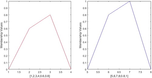
This critical assessment ascertains that the present approach is highly efficient enough to prevail over all the inadequacies of the existing approaches. Furthermore, the present approach can also measure similarity between GFNs with different left and right heights. For instance, consider the profile 23 is $\xi =[2,4,6,8;0.6,0.8]$ & $\eta =[2,4,6,8;0.8,1]$ presented in Figure 25 and profile 24 is $\xi =[1,2,3,4;0.6,0.8]$ & $\eta =[5,6,7,8;0.8,1]$ presented in Figure 26, then the SM of the profile 23 is 0.9984 and profile 24 is 0.6853. All the above mentioned approaches are unable to evaluate SM except the work of Chutia and Gogoi (2018).

5. Application of the proposed SM approach in MCDM problem

Here, applicability and novelty of the proposed Dice SM approach has been showcased by solving MCDM problem.

An MCDM is a technique to choose best alternative or to evaluate preference ordering of alternatives among a profile of alternatives based on preallotted multi criteria. In MCDM problems, two types of criteria are taken into consideration, first one is the criteria that to be maximized called the profit/benefit criteria and the later one is the criteria that to be minimized called cost criteria. Usually, a criteria of the later type can be converted into profit/benefit criteria (Zizovic, Damljanovic, & Zizovic, 2017). On the other hand, an ideal solution to a MCDM problem would maximize all the profit criteria and minimize all the cost criteria (Xu & Yang, 2001).

Let’s consider $A=\{A_1,A_2,\dots ,A_n\}$ and $C=\{C_1,C_2,C_3,\dots ,C_m\}$ are profiles of alternatives and criteria, respectively. As the criteria in MCDM problems are uncertain in nature, therefore, the representation of uncertain criteria are taken as GTFNs of the type $\chi =\left[{\chi }_{ij1},{\chi }_{ij2},{\chi }_{ij3};{\omega }_{ij}\right]$ where $i=1,2,\dots ,n;j=1,2,\dots ,m;$ ${\chi }_{\mathit{ijp}}\in \mathbb{R};$ $p=1,2,3.$ and ${\chi }_{ij1}\le {\chi }_{ij2}\le {\chi }_{ij3}.$ Here ω_ij is the height of the GTFN $\chi .$

Then, a fuzzy judgement matrix $J_{ij}=[{\Upsilon }_{ij}]$ can be constructed based on these criteria and alternatives. The profile of criteria is divided into two profiles, viz., profit/benefit criteria ${\Delta }^B$ and cost criteria ${\Delta }^C,$ respectively. An approach to evaluate best alternative or preference ordering of the alternatives is presented here.

Step-1:

Consider ${\Delta }^B$ and ${\Delta }^C.$ Then, the judgement matrix $J_{ij}={[{\Upsilon }_{ij}]}_{n\times m}=\left[{\Theta }_{ij1},{\Theta }_{ij2},{\Theta }_{ij3};{\omega }_{ij}\right]$ is to be normalized into ${\overline{J}}_{ij}={[{\Phi }_{ij}]}_{n\times m}=\left[{\Phi }_{ij1},{\Phi }_{ij2},{\Phi }_{ij3};{\omega }_{ij}^{\prime }\right]$ first using the following method (Xu et al., 2010).

(a) For profit criteria $(i.e.,C_j\in {\Delta }^B)$ $$\{\begin{array}{c}{\Phi }_{ij1}={\Theta }_{ij1}/\underset{i}{m}ax\left\{{\Theta }_{ij3}\right\}\hfill \\ {\Phi }_{ij2}={\Theta }_{ij2}/\underset{i}{m}ax\left\{{\Theta }_{ij2}\right\}\hfill \\ {\Phi }_{ij3}={\Theta }_{ij3}/\underset{i}{m}ax\left\{{\Theta }_{ij1}\right\}\wedge 1\hfill \\ {\omega }_{ij}^{\prime }={\omega }_{ij}/\underset{i}{m}ax\left\{{\omega }_{ij}\right\}\hfill \end{array}$$

(b) For cost criteria $(i.e.,C_j\in {\Delta }^C)$ $$\{\begin{array}{c}{\Phi }_{ij1}=\underset{i}{m}in({\Theta }_{ij1})/{\Theta }_{ij3}\hfill \\ {\Phi }_{ij2}=\underset{i}{m}in({\Theta }_{ij2})/{\Theta }_{ij2}\hfill \\ {\Phi }_{ij3}=\underset{i}{m}in({\Theta }_{ij3})/{\Theta }_{ij1}\wedge 1\hfill \\ {\omega }_{ij}^{\prime }=\underset{i}{m}in({\omega }_{ij})/{\omega }_{ij}\}\hfill \end{array}$$

Step-2:

To evaluate best alternative, it is needed to evaluate the SM of the available alternatives with an ideal alternative. For this purpose, consider the ideal alternative $A^{*}$ as $q_j^{*}=[1,1,1,1;1].$

Step-3:

Then, calculate the similarity measure of alternatives A_i and the ideal alternative $A^{*}$ using the technique (9) $$D_S(A_i,A^{)}=\frac{1}{m}\stackrel{m}{\sum _{j=1}}\frac{2[{\Phi }_{ij1}+2{\Phi }_{ij2}+{\Phi }_{ij3}+|{\omega }_{ij}^{\prime }-1\left|\right|{\omega }_{ij}^{\prime }-1\left|\right]}{{\Phi }_{ij1}^2+2{\Phi }_{ij2}^2+{\Phi }_{ij3}^2+4+2|{\omega }_{ij}^{\prime }-1{|}^2}$$(9) this is the SM of each alternative based on all criteria. Preference of ordering of alternatives or the best alternative among the set of alternatives can be evaluated via these evaluated similarity values, the maximum similarity value indicates the best alternative and accordingly preference preference ordering of alternatives can be obtained.

5.1. Numerical illustration

Supposed a company is launching a novel product and therefore, the company has a set four alternatives $A_1,A_2,A_3$ and A₄ and to choose best alternatives or preference ordering of alternatives the company set the the criteria viz., C₁: funding total, C₂: predictable net earning, C₃: Investment return and C₄: Investment lost. It should be noted that among of these four criteria the profit/benefit criteria are C₂ and C₃ and cost criteria are C₁ and C₄, respectively. The judgement matrix is given in Table 3).

Table 3. Judgement matrix $J_{ij}=[{\Theta }_{ij}].$

Alternatives	C1	C2	C3	C4
A1	[5,6,6,7;0.8]	[3,4,4,5;0.5]	[4,5,5,6;0.6]	[0.4,0.5,0.5,0.6;0.2]
A2	[9,10,10,11;0.9]	[5,5.5,5.5,6;0.7]	[5,5.5,5.5,6;0.5]	[1.4,1.7,1.7,2;0.4]
A3	[5,5.5,5.5,6;0.4]	[4,4.5,4.5,5;0.5]	[3,3.5,3.5,4;0.3]	[0.8,0.9,0.9,1;0.4]
A4	[8,9,9,10;0.3]	[3,3.5,3.5,4;0.4]	[3,3.5,3.5,4;0.4]	[0.5,0.6,0.6,0.7;0.3]

Step-1 Here $C_2 \&C_3$ profit criteria and $C_1 \& C_4$ are cost criteria, normalizing D_ij we have ${\overline{D}}_{ij}$ and presented in Table 4.

Table 4. Normalized judgement matrix ${\overline{J}}_{ij}.$

Alts	C1	C2	C3	C4
A1	[0.71,0.92,0.92,1.00;0.37]	[0.50,0.73,0.73,1.00;0.71]	[0.67,0.91,0.91,1.00;1]	[0.67,1.00,1.00,1.00;1]
A2	[0.45,0.55,0.55,0.67;0.33]	[0.83,1.00,1.00,1.00;1]	[0.83,1.00,1.00,1.00;0.83]	[0.20,0.29,0.29,0.43;0.50]
A3	[0.83,1.00,1.00,1.00;0.75]	[0.67,0.82,0.82,1.00;0.71]	[0.50,0.64,0.64,0.80;0.50]	[0.40,0.56,0.56,0.75;0.50]
A4	[0.50,0.61,0.61,0.75;1]	[0.50,0.64,0.64,0.80;0.57]	[0.50,0.64,0.64,0.80;1;0.67]	[0.57,0.83,0.83,1.00;0.67]

Step-2 To evaluate SM of all the available alternatives with an ideal one, it is adopted here that the ideal alternative $A^{*}$ as $q_j^{*}=[1,1,1;1].$

Step-3 Evaluate $D_S(A_i,A^{*})$ using equation (9)(9) $$D_S(A_i,A^{)}=\frac{1}{m}\stackrel{m}{\sum _{j=1}}\frac{2[{\Phi }_{ij1}+2{\Phi }_{ij2}+{\Phi }_{ij3}+|{\omega }_{ij}^{\prime }-1\left|\right|{\omega }_{ij}^{\prime }-1\left|\right]}{{\Phi }_{ij1}^2+2{\Phi }_{ij2}^2+{\Phi }_{ij3}^2+4+2|{\omega }_{ij}^{\prime }-1{|}^2}$$(9) , we have

$D_S(A_1,A^{*})=0.9737,S(A_2,A^{*})=0.8641$ $S(A_3,A^{*})=0.9361$ and $S(A_4,A^{*})=0.9169.$

As SM of A₁ with the ideal alternative $A^{*}$ is found to be maximum, so A₁ is the required best alternative and consequently, have the required preference ordering $A_1>A_3>A_4>A_2.$

6. Conclusion

To solve MCDM problems under fuzzy environment, SM plays crucial role. although a handful numbers of attempts were made to proposed SM, however, most of the existing approaches have some sort of limitations and more often produce irrational output. Therefore, in this paper, a novel dice similarity between has been devised for evaluating similarity value between GFNs for same and different support as well. It is pragmatic that the proposed approach is straightforward, more competent, commonsensical, technically sound method for implementation. A comparative study has been performed which established that the present has the capability to overcome the limitations of the existing approaches. Furthermore, the applicability and validity has been showcased by solving a FMCDM problem. However, the present approach has a miniature limitation that when SM is evaluated between crisp valued fuzzy number [0,0,0,0;w] and any arbitrary GFN, it shows counter-intuitive behaviour (as discussed in section 3.3). As an extension of this work, the deficiency of the present work may be addressed directly and a new method may be proposed in such a way that SM can be evaluated within a single framework.

Acknowledgement

Author would like to thank Prof. Radko Mesiar for his guidance in revising the paper.

No potential conflict of interest was reported by the author(s).

Disclosure statement

Correction Statement

This article has been republished with minor changes. These changes do not impact the academic content of the article.

Appendix

Figure 3. Profile-1.

Figure 4. Profile-2.

Figure 5. Profile-3.

Figure 6. Profile-4.

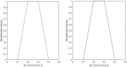
Figure 7. Profile-5.

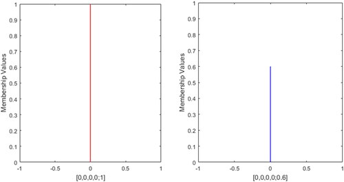
Figure 8. Profile-6.

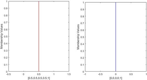
Figure 9. Profile-7.

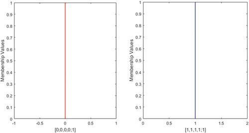
Figure 10. Profile-8.

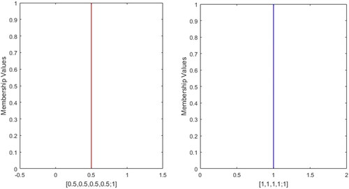
Figure 11. Profile-9.

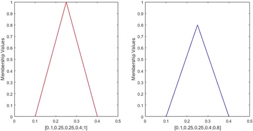
Figure 12. Profile-10.

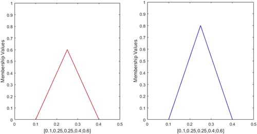
Figure 13. Profile-11.

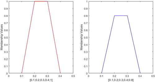
Figure 14. Profile-12.

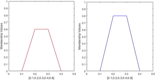
Figure 15. Profile-13.

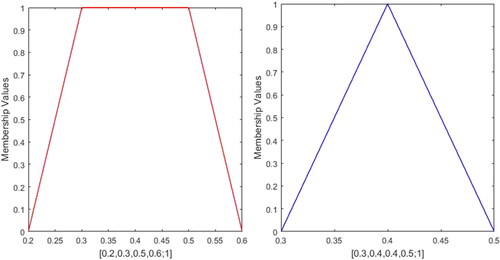
Figure 16. Profile-14.

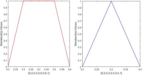
Figure 17. Profile-15.

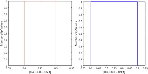
Figure 18. Profile-16.

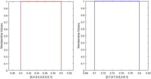
Figure 19. Profile-17.

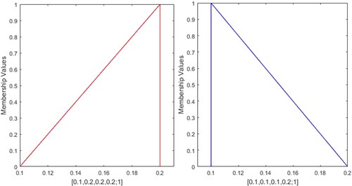
Figure 20. Profile-18.

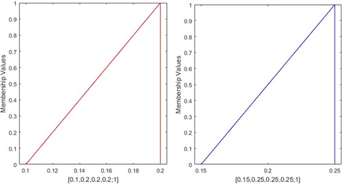
Figure 21. Profile-19.

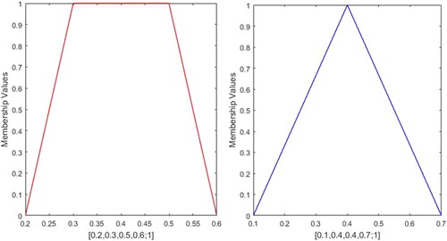
Figure 22. Profile-20.

Figure 23. Profile-21.

Figure 24. Profile-22.

Figure 25. Profile-23.

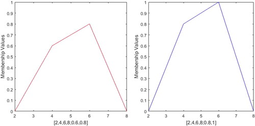
Figure 26 Profile-24.

References

- Ahmad, S. A. S., Mohamad, D., Sulaiman, N. H., Shariff, J. M., & Abdullah, K. (2018, June). A distance and set theoretic-based similarity measure for generalized trapezoidal fuzzy numbers. In AIP Conference Proceedings (Vol. 1974, No. 1, p. 020043). AIP Publishing.
- Baccour, L. (2018). New intuitionistic fuzzy similarity and distance measures applied to multi-criteriadecision making. Mechatronic Systems and Control, 46(1), 1–7.
- Beg, I., & Rashid, T. (2017). A fuzzy similarity measure based on equivalence relation with application in cluster analysis. International Journal of Computers and Applications, 39(3), 148–154. doi:10.1080/1206212X.2017.1309220
- Chen, S. H. (1985). Ranking fuzzy numbers with maximizing set and minimizing set. Fuzzy Sets and Systems, 17(2), 113–129. doi:10.1016/0165-0114(85)90050-8
- Chen, S. J., & Chen, S. M. (2001, December). A new method to measure the similarity between fuzzy numbers. In 10th IEEE International Conference on Fuzzy Systems (Cat. No. 01CH37297) (Vol. 3, pp. 1123–1126). IEEE.
- Chen, S. J., & Hwang, C. L. (1992). Fuzzy multiple attribute decision making methods. In Shu-Jen Chen, Ching-Lai Hwang (Eds.), Fuzzy multiple attribute decision making (pp. 289–486). Berlin, Heidelberg: Springer.
- Chen, S. M. (1996). New methods for subjective mental workload assessment and fuzzy risk analysis. Cybernetics and Systems, 27(5), 449–472. doi:10.1080/019697296126417
- Chen, S. M., Munif, A., Chen, G. S., Liu, H. C., & Kuo, B. C. (2012). Fuzzy risk analysis based on ranking generalized fuzzy numbers with different left heights and right heights. Expert Systems with Applications, 39(7), 6320–6334. doi:10.1016/j.eswa.2011.12.004
- Chutia, R., & Gogoi, M. K. (2018). Fuzzy risk analysis in poultry farming based on a novel similarity measure of fuzzy numbers. Applied Soft Computing, 66, 60–76. doi:10.1016/j.asoc.2018.02.008
- Dhivya, J., & Sridevi, B. (2019). A novel similarity measure between intuitionistic fuzzy sets based on the mid points of transformed triangular fuzzy numbers with applications to pattern recognition and medical diagnosis. Applied Mathematics-A Journal of Chinese Universities, 34(2), 229–252. doi:10.1007/s11766-019-3708-x
- Dice, L. R. (1945). Measures of the amount of ecologic association between species. Ecology, 26(3), 297–302. doi:10.2307/1932409
- Dutta, P., & Hazarika, G. C. (2017). Construction of families of probability boxes and corresponding membership functions at different fractiles. Expert Systems, 34(3), e12202. doi:10.1111/exsy.12202
- Fei, L., Wang, H., Chen, L., & Deng, Y. (2019). A new vector valued similarity measure for intuitionistic fuzzy sets based on OWA operators. Iranian Journal of Fuzzy Systems, 16(3), 113–126.
- Garg, H. (2018). An improved cosine similarity measure for intuitionistic fuzzy sets and their applications to decision-making process. Hacettepe Journal of Mathematics and Statistics, 47(6), 1578–1594. doi:10.15672/HJMS.2017.510
- Hejazi, S. R., Doostparast, A., & Hosseini, S. M. (2011). An improved fuzzy risk analysis based on a new similarity measures of generalized fuzzy numbers. Expert Systems with Applications, 38(8), 9179–9185. doi:10.1016/j.eswa.2011.01.101
- Hesamian, G. (2017). Fuzzy similarity measure based on fuzzy sets. Control and Cybernetics, 46, 71–86.
- Hesamian, G., & Chachi, J. (2017). On similarity measures for fuzzy sets with applications to pattern recognition, decision making, clustering, and approximate reasoning. Journal of Uncertain Systems, 11(1), 35–48.
- Hsieh, C. H. (1999). (1999). Similarity of generalized fuzzy numbers with graded mean integration representation. Proc. 8th Int. Fuzzy Systems Association World Congr, 2, 551–555.
- Jaccard, P. (1901). Distribution de la flore alpine dans le bassin des Dranses et dans quelques régions voisines. Bull Soc Vaudoise Sci Nat, 37, 241–272.
- Khorshidi, H. A., & Nikfalazar, S. (2017). An improved similarity measure for generalized fuzzy numbers and its application to fuzzy risk analysis. Applied Soft Computing, 52, 478–486. doi:10.1016/j.asoc.2016.10.020
- Lee, H. S. (2002). Optimal consensus of fuzzy opinions under group decision making environment. Fuzzy Sets and Systems, 132(3), 303–315. doi:10.1016/S0165-0114(02)00056-8
- Liu, D., Chen, X., & Peng, D. (2018). Cosine similarity measure between hybrid intuitionistic fuzzy sets and its application in medical diagnosis. Computational and Mathematical Methods in Medicine, 2018, 1–7. doi:10.1155/2018/3146873
- Luo, M., & Liang, J. (2018). A novel similarity measure for interval-valued intuitionistic fuzzy sets and its applications. Symmetry, 10(10), 441. doi:10.3390/sym10100441
- Mo, H., & Deng, Y. (2018). A new MADA methodology based on D numbers. International Journal of Fuzzy Systems, 20(8), 2458–2469.
- Patra, K., & Mondal, S. K. (2015). Fuzzy risk analysis using area and height based similarity measure on generalized trapezoidal fuzzy numbers and its application. Applied Soft Computing, 28, 276–284. doi:10.1016/j.asoc.2014.11.042
- Peng, X., & Garg, H. (2019). Multiparametric similarity measures on Pythagorean fuzzy sets with applications to pattern recognition. Applied Intelligence, 49(12), 4058–4096. doi:10.1007/s10489-019-01445-0
- Phan, T. T. H., Bigand, A., & Caillault, E. P. (2018). A new fuzzy logic-based similarity measure applied to large gap imputation for uncorrelated multivariate time series. Applied Computational Intelligence and Soft Computing, 2018, 1–15. doi:10.1155/2018/9095683
- Salton, G., & McGill, M.J. (1987). Introduction to Modern Information Retrieval. New York, NY: McGraw-Hill.
- Singhal, N., Verma, A., & Chouhan, U. (2018). An application of similarity measure of fuzzy soft sets in verndor selection problem. Materials Today: Proceedings, 5(2), 3987–3993. doi:10.1016/j.matpr.2017.11.657
- Song, Y., Wang, X., Quan, W., & Huang, W. (2019). A new approach to construct similarity measure for intuitionistic fuzzy sets. Soft Computing, 23(6), 1985–1998. doi:10.1007/s00500-017-2912-0
- Tourad, M. C., & Abdali, A. (2018). An intelligent similarity model between generalized trapezoidal fuzzy numbers in large scale. International Journal of Fuzzy Logic and Intelligent Systems, 18(4), 303–315. doi:10.5391/IJFIS.2018.18.4.303
- Wang, X., Wang, J., & Chen, X. (2016). Fuzzy multi-criteria decision making method based on fuzzy structured element with incomplete weight information. Iranian Journal of Fuzzy Systems, 13(2), 1–17.
- Wei, G. (2018). Some similarity measures for picture fuzzy sets and their applications. Iranian Journal of Fuzzy Systems, 15(1), 77–89.
- Wei, S. H., & Chen, S. M. (2009). A new approach for fuzzy risk analysis based on similarity measures of generalized fuzzy numbers. Expert Systems with Applications, 36(1), 589–598. doi:10.1016/j.eswa.2007.09.033
- Xu, L., & Yang, J. B. (2001). Introduction to multi-criteria decision making and the evidential reasoning approach (pp. 1–21). Manchester: Manchester School of Management.
- Xu, Z., Shang, S., Qian, W., & Shu, W. (2010). A method for fuzzy risk analysis based on the new similarity of trapezoidal fuzzy numbers. Expert Systems with Applications, 37(3), 1920–1927. doi:10.1016/j.eswa.2009.07.015
- Ye, J. (2011). Cosine similarity measures for intuitionistic fuzzy sets and their applications. Mathematical and Computer Modelling, 53(1–2), 91–97. doi:10.1016/j.mcm.2010.07.022
- Ye, J. (2012). The Dice similarity measure between generalized trapezoidal fuzzy numbers based on the expected interval and its multicriteria group decision-making method. Journal of the Chinese Institute of Industrial Engineers, 29(6), 375–382. doi:10.1080/10170669.2012.710879
- Yong, D., Wenkang, S., Feng, D., & Qi, L. (2004). A new similarity measure of generalized fuzzy numbers and its application to pattern recognition. Pattern Recognition Letters, 25(8), 875–883. doi:10.1016/j.patrec.2004.01.019
- Zadeh, L. A. (1965). Fuzzy sets. Information and Control, 8(3), 338–353. doi:10.1016/S0019-9958(65)90241-X
- Zadeh, L. A. (1975). The concept of a linguistic variable and its application to approximate reasoning–I. Information Sciences, 8(3), 199–249. doi:10.1016/0020-0255(75)90036-5
- Zizovic, M. M., Damljanovic, N., & Zizovic, M. R. (2017). Multi-criteria decision making method for models with the dominant criterion. Filomat, 31(10), 2981–2989. doi:10.2298/FIL1710981Z