Stability analysis for a rational difference equation

Abstract

Most qualitative behaviours of difference equations are rapidly investigated nowadays. This can be attributed to the fact that it is often sophisticated to construct the exact solutions of most difference equations. This article is written to analyse the local stability, global attractor and the boundedness of the solution of the seventh order difference equation given by

$x_{n+1}=c_1{x}_{n-1}-\frac{c_2{x}_{n-1}{x}_{n-4}}{c_3{x}_{n-4}+c_4{x}_{n-6}},n=0,1,\dots ,$

where the coefficients $c_i,\mathit{for}\mathit{all}i=1,\dots ,4,$ are supposed to be positive real numbers and the initial conditions $x_i\mathit{for}\mathit{all}i=-6,-5,\dots ,0,$ are arbitrary non-zero real numbers. Under some suitable conditions, the stability, boundedness and a special case equation from the considered equation are presented in 2 D figures.

Keywords:

• Attractivity
• boundedness
• equilibrium
• recursive equation
• stability

Mathematics Subject Classification:

• 39A10

1. Introduction

The theory of difference equations has attained its popularity in recent decades due to its use in modelling most real life phenomena. It is worth mentioning that the difference equations are utilized in modelling some problems such as biological, physical, economical problems and several others. In order to understand the long behaviour of such models, one can study the qualitative and quantitative behaviours of these problem. This can be easily achieved by exploring the stability, periodicity and boundedness of the solutions.

Most researchers are mainly interested in studying difference equations of low order. As a result, simple analysis is required to investigate such equations. However, considering difference equations of high order leads to a very interesting, powerful and rigorous analysis. In this work, we present local and global stability for seventh order difference equations which can be generalized for other equations with higher orders. Indeed, such equations appear naturally as discrete analogues for differential equations which model a massive number of natural phenomena (Agarwal, 1992; Fisher, 1984; Kocic & Ladas, 1993). Thus, we are excited to study such proposed equations.

Recently, many authors have comprehensively analysed some relevant properties. Among some existing articles, we mention Moaaz, Chalishajar, and Bazighifan (2019) analysed a general class of difference equations on the form $$J_{n+1}=f(J_n,J_{n-1}),$$ and presented suitable conditions for the local asymptotic stability and investigated the periodic solutions of these equations. In 1999, Amleh et al. (Amleh, Grove, Georgiou, & Ladas, 1999) explored the global attractivity, the periodic character and the boundedness nature of the positive solutions of the recursive equation (1) $$x_{n+1}=\alpha +\frac{x_{n-1}}{x_n},\alpha \ge 0.$$(1)

Equation (1)(1) $$x_{n+1}=\alpha +\frac{x_{n-1}}{x_n},\alpha \ge 0.$$(1) was also studied by Hamza (2006) for negative $\alpha .$ Almatrafi and Alzubaidi (2019) concentrated on constructing the asymptotic stability, periodicity and boundedness of the rational difference equation $$x_{n+1}=c_1{x}_{n-3}+\frac{c_2{x}_{n-3}}{c_3{x}_{n-3}-c_4{x}_{n-7}}.$$

In Almatrafi (2019), the author presented the forms of solutions of the system $$x_{n+1}=\frac{x_{n-1}{y}_{n-3}}{y_{n-1}\left(-1-x_{n-1}{y}_{n-3}\right)},y_{n+1}=\frac{y_{n-1}{x}_{n-3}}{x_{n-1}\left(\pm 1\pm y_{n-1}{x}_{n-3}\right)},n=0,1,\dots ,$$

Garić-Demirović, Nurkanović, and Nurkanović (2017) analysed the periodicity and stability of the solution of the equation $$x_{n+1}=\frac{A{x}_n^2+B{x}_n{x}_{n-1}+C{x}_{n-1}^2}{a{x}_n^2+b{x}_n{x}_{n-1}+c{x}_{n-1}^2}.$$

Several articles are devoted to show the qualitative behaviours of some difference equations. Among these are refs. (Abdelrahman, 2019; Abdelrahman, Chatzarakis, Tongxing, & Osama, 2018; Almatrafi, Elsayed, & Alzahrani, 2019; Almatrafi & Elsayed, 2018; Almatrafi, Elsayed, & Alzahrani, 2018; Belhannache, Touafek, & Abo-Zeid, 2016; Elabbasy, El-Metawally, & Elsayed, 2008; El-Moneam & Zayed, 2014; Khaliq & Hassan, 2018; Khyat, & Kulenović, 2017; Kocic & Ladas, 1993; Kostrov & Kudlak, 2016; Liu, Li, Han, & Zhong, 2018; Moranjkić & Nurkanović, 2017; Saleh & Aloqeili, 2005; Simsek, Cinar, & Yalcinkaya, 2006).

It is the fundamental aim of this work to discuss some mathematical aspects, for example the stability and boundedness, for the following recursive equation: (2) $$x_{n+1}=c_1{x}_{n-1}-\frac{c_2{x}_{n-1}{x}_{n-4}}{c_3{x}_{n-4}+c_4{x}_{n-6}},n=0,1,\dots ,$$(2) where the coefficients $c_i,\mathit{for}\mathit{all}i=1,\dots ,4,$ are positive real numbers. It is to be noted that the initial data is arbitrarily real numbers. Furthermore, this paper presents exact and numerical solutions to a special case from Equation (2)(2) $$x_{n+1}=c_1{x}_{n-1}-\frac{c_2{x}_{n-1}{x}_{n-4}}{c_3{x}_{n-4}+c_4{x}_{n-6}},n=0,1,\dots ,$$(2) .

2. Local stability of the equilibrium point

The local stability in the neighbourhood of the fixed point is extensively highlighted in this section. We provide special conditions under which the equilibrium point is locally asymptotically stable. The equilibrium point is given by $$\overline{x}=c_1\overline{x}-\frac{c_2{\overline{x}}^2}{c_3\overline{x}+c_4\overline{x}}.$$

If $\frac{c_2}{c_3+c_4}+1\ne c_1,$ then the unique equilibrium point is given by $\overline{x}=0.$ We now introduce a new function to obtain the stability of Equation (2)(2) $$x_{n+1}=c_1{x}_{n-1}-\frac{c_2{x}_{n-1}{x}_{n-4}}{c_3{x}_{n-4}+c_4{x}_{n-6}},n=0,1,\dots ,$$(2) . Define a function $g:{(0,\infty )}^3\to (0,\infty )$ by (3) $$g(\varphi ,\psi ,\theta )=c_1\varphi -\frac{c_2\varphi \psi }{c_3\psi +c_4\theta }.$$(3)

Hence, (4) $$\frac{\partial g(\varphi ,\psi ,\theta )}{\partial \varphi }=c_1-\frac{c_2\psi }{(c_3\psi +c_4\theta )},$$(4) (5) $$\frac{\partial g(\varphi ,\psi ,\theta )}{\partial \psi }=-\frac{c_2{c}_4\varphi \theta }{{(c_3\psi +c_4\theta )}^2},$$(5) (6) $$\frac{\partial g(\varphi ,\psi ,\theta )}{\partial \theta }=\frac{c_2{c}_4\varphi \psi }{{(c_3\psi +c_4\theta )}^2}.$$(6)

The following step is embodied in evaluating Equations (4)(4) $$\frac{\partial g(\varphi ,\psi ,\theta )}{\partial \varphi }=c_1-\frac{c_2\psi }{(c_3\psi +c_4\theta )},$$(4) , (5)(5) $$\frac{\partial g(\varphi ,\psi ,\theta )}{\partial \psi }=-\frac{c_2{c}_4\varphi \theta }{{(c_3\psi +c_4\theta )}^2},$$(5) and Equation (6)(6) $$\frac{\partial g(\varphi ,\psi ,\theta )}{\partial \theta }=\frac{c_2{c}_4\varphi \psi }{{(c_3\psi +c_4\theta )}^2}.$$(6) at $\overline{x}.$ That is $$\begin{array}{c}\frac{\partial g(\overline{x},\overline{x},\overline{x})}{\partial \varphi }=c_1-\frac{c_2\overline{x}}{(c_3\overline{x}+c_4\overline{x})}=c_1-\frac{c_2}{c_3+c_4}:=-q_1,\\ \frac{\partial g(\overline{x},\overline{x},\overline{x})}{\partial \psi }=-\frac{c_2{c}_4{\overline{x}}^2}{{(c_3\overline{x}+c_4\overline{x})}^2}=-\frac{c_2{c}_4}{{(c_3+c_4)}^2}:=-q_2,\\ \frac{\partial g(\overline{x},\overline{x},\overline{x})}{\partial \theta }=\frac{c_2{c}_4{\overline{x}}^2}{{(c_3\overline{x}+c_4\overline{x})}^2}=\frac{c_2{c}_4}{{(c_3+c_4)}^2}:=-q_3.\end{array}$$

Thus, the linearized equation of Equation (2)(2) $$x_{n+1}=c_1{x}_{n-1}-\frac{c_2{x}_{n-1}{x}_{n-4}}{c_3{x}_{n-4}+c_4{x}_{n-6}},n=0,1,\dots ,$$(2) around $\overline{x}$ can be presented as follows: $$T_{n+1}+q_1{T}_{n-1}+q_2{T}_{n-4}+q_3{T}_{n-6}=0.$$

Theorem 1.

Let $c_2<c_1(c_3+c_4),$ and assume that $$c_2(c_4-c_3)<(1-c_1){(c_3+c_4)}^2.$$

Then, the equilibrium point of Equation (2)(2) $$x_{n+1}=c_1{x}_{n-1}-\frac{c_2{x}_{n-1}{x}_{n-4}}{c_3{x}_{n-4}+c_4{x}_{n-6}},n=0,1,\dots ,$$(2) is locally asymptotically stable.

Proof.

According to Theorem A in (Elabbasy et al., 2008), the local stability of the equilibrium point occurs if (7) $$\left|q_1\right|+\left|q_2\right|+\left|q_3\right|<1,$$(7)

Substituting $q_i,i=1,2,3,$ into Equation (7)(7) $$\left|q_1\right|+\left|q_2\right|+\left|q_3\right|<1,$$(7) leads to (8) $$\left|-\left(c_1-\frac{c_2}{c_3+c_4}\right)\right|+\left|\frac{c_2{c}_4}{{(c_3+c_4)}^2}\right|+\left|-\left(\frac{c_2{c}_4}{{(c_3+c_4)}^2}\right)\right|<1.$$(8)

If $c_2<c_1(c_3+c_4),$ then Equation (8)(8) $$\left|-\left(c_1-\frac{c_2}{c_3+c_4}\right)\right|+\left|\frac{c_2{c}_4}{{(c_3+c_4)}^2}\right|+\left|-\left(\frac{c_2{c}_4}{{(c_3+c_4)}^2}\right)\right|<1.$$(8) leads to $$c_1{(c_3+c_4)}^2-c_2(c_3+c_4)+2c_2{c}_4<{(c_3+c_4)}^2,$$ which can be reduced to $$c_2(c_4-c_3)<(1-c_1){(c_3+c_4)}^2.$$

Theorem 2.

Suppose that $c_2>c_1(c_3+c_4),$ and let $$c_2(c_3+3c_4)<(1+c_1){(c_3+c_4)}^2.$$

Then, the equilibrium point of Equation (2)(2) $$x_{n+1}=c_1{x}_{n-1}-\frac{c_2{x}_{n-1}{x}_{n-4}}{c_3{x}_{n-4}+c_4{x}_{n-6}},n=0,1,\dots ,$$(2) is locally asymptotically stable.

Proof.

The proof is similar to the proof of Theorem (1). Hence, it omitted.

3. Analysis of global stability

This section is included to illustrate the global attractivity of the equilibrium point. The investigation of this part is established by employing Theorem B in (Elsayed, 2010).

Theorem 3.

Assume that $c_1>\frac{c_2\psi }{c_3\psi +c_4\theta }.$ Then, the equilibrium point of Equation (2) is a global attractor if $c_1<1.$

Proof.

Let $r,s\in \mathbb{R}$ and assume that $g:{\left[r,s\right]}^3\to \left[r,s\right]$ is a function defined by Equation (3)$$\overline{x}=c_1\overline{x}-\frac{c_2{\overline{x}}^2}{c_3\overline{x}+c_4\overline{x}}.$$. Then, it can be apparently noted from Equations (4)(4) $$\frac{\partial g(\varphi ,\psi ,\theta )}{\partial \varphi }=c_1-\frac{c_2\psi }{(c_3\psi +c_4\theta )},$$(4) , (5)(5) $$\frac{\partial g(\varphi ,\psi ,\theta )}{\partial \psi }=-\frac{c_2{c}_4\varphi \theta }{{(c_3\psi +c_4\theta )}^2},$$(5) and Equation (6)(6) $$\frac{\partial g(\varphi ,\psi ,\theta )}{\partial \theta }=\frac{c_2{c}_4\varphi \psi }{{(c_3\psi +c_4\theta )}^2}.$$(6) that g is increasing in $\varphi$ and in θ and decreasing in $\psi .$ Theorem B in (Elsayed, 2010) requires a solution (say $(\zeta ,\eta )$) to the following system: $$\zeta =g(\zeta ,\eta ,\zeta ),\eta =g(\eta ,\zeta ,\eta ).$$

Or, $$\begin{array}{c}\zeta =g(\zeta ,\eta ,\zeta )=c_1\zeta -\frac{c_2\zeta \eta }{c_3\eta +c_4\zeta },\\ \eta =g(\eta ,\zeta ,\eta )=c_1\eta -\frac{c_2\eta \zeta }{c_3\zeta +c_4\eta },\end{array}$$ which can be expanded as follows: (9) $$c_3\zeta \eta +c_4{\zeta }^2=c_1{c}_3\zeta \eta +c_1{c}_4{\zeta }^2-c_2\zeta \eta ,$$(9) (10) $$c_3\zeta \eta +c_4{\eta }^2=c_1{c}_3\zeta \eta +c_1{c}_4{\eta }^2-c_2\zeta \eta .$$(10)

Now, we subtract Equation (10)(10) $$c_3\zeta \eta +c_4{\eta }^2=c_1{c}_3\zeta \eta +c_1{c}_4{\eta }^2-c_2\zeta \eta .$$(10) from Equation (9)(9) $$c_3\zeta \eta +c_4{\zeta }^2=c_1{c}_3\zeta \eta +c_1{c}_4{\zeta }^2-c_2\zeta \eta ,$$(9) to obtain $$c_4({\zeta }^2-{\eta }^2)=c_1{c}_4({\zeta }^2-{\eta }^2),$$ which can be rearranged as $$c_4({\zeta }^2-{\eta }^2)[1-c_1]=0.$$

Therefore, if $c_1<1,$ then $\zeta =\eta .$ As a result, Theorem B (Elsayed, 2010) concludes that the equilibrium point is a global attractor.

Theorem 4.

Assume that $c_1<\frac{c_2\psi }{c_3\psi +c_4\theta }.$ Then, the equilibrium point of Equation (2)(2) $$x_{n+1}=c_1{x}_{n-1}-\frac{c_2{x}_{n-1}{x}_{n-4}}{c_3{x}_{n-4}+c_4{x}_{n-6}},n=0,1,\dots ,$$(2) is a global attractor if $c_4+c_1{c}_2\ne c_2.$

Proof.

The proof is similar to the previous proof. Thus, it is omitted.

4. Exact solution to $x_{n+1}=x_{n-1}-\frac{x_{n-1}{x}_{n-4}}{x_{n-4}+x_{n-6}}$

This section provides sophisticated forms of solutions to the following rational recursive relation: (11) $$x_{n+1}=x_{n-1}-\frac{x_{n-1}{x}_{n-4}}{x_{n-4}+x_{n-6},},$$(11) where the initial data as shown previously.

Theorem 5.

Let ${\left\{x_n\right\}}_{n=-6}^{\infty }$ be a solution to Equation (11)(11) $$x_{n+1}=x_{n-1}-\frac{x_{n-1}{x}_{n-4}}{x_{n-4}+x_{n-6},},$$(11) and assume that $x_{-6}=a,x_{-5}=b,x_{-4}=c,x_{-3}=d,x_{-2}=e,x_{-1}=r,x_0=k$. Then, for $n=0,1,\dots ,$ we have $$\begin{array}{c}{x}_{10n-6}=a\underset{i=0}{\prod ^{n-1}}\frac{(F_{2i}d+F_{2i+1}b)(F_{2i}r+F_{2i+1}d)(F_{2i-1}k+F_{2i}e)(F_{2i-1}c+F_{2i}a)(F_{2i-1}e+F_{2i}c)}{(F_{2i+1}d+F_{2i+2}b)(F_{2i+1}r+F_{2i+2}d)(F_{2i}k+F_{2i+1}e)(F_{2i}c+F_{2i+1}a)(F_{2i}e+F_{2i+1}c)},\\ x_{10n-5}=b\underset{i=0}{\prod ^{n-1}}\frac{(F_{2i}k+F_{2i+1}e)(F_{2i}e+F_{2i+1}c)(F_{2i}c+F_{2i+1}a)(F_{2i-1}d+F_{2i}b)(F_{2i-1}r+F_{2i}d)}{(F_{2i+1}k+F_{2i+2}e)(F_{2i+1}e+F_{2i+2}c)(F_{2i+1}c+F_{2i+2}a)(F_{2i}d+F_{2i+1}b)(F_{2i}r+F_{2i+1}d)},\\ x_{10n-4}=c\underset{i=0}{\prod ^{n-1}}\frac{(F_{2i+1}c+F_{2i+2}a)(F_{2i}d+F_{2i+1}b)(F_{2i}r+F_{2i+1}d)(F_{2i-1}k+F_{2i}e)(F_{2i-1}e+F_{2i}c)}{(F_{2i+2}c+F_{2i+3}a)(F_{2i+1}d+F_{2i+2}b)(F_{2i+1}r+F_{2i+2}d)(F_{2i}k+F_{2i+1}e)(F_{2i}e+F_{2i+1}c)},\\ x_{10n-3}=d\underset{i=0}{\prod ^{n-1}}\frac{(F_{2i+1}d+F_{2i+2}b)(F_{2i}k+F_{2i+1}e)(F_{2i}e+F_{2i+1}c)(F_{2i}c+F_{2i+1}a)(F_{2i-1}r+F_{2i}d)}{(F_{2i+2}d+F_{2i+3}b)(F_{2i+1}k+F_{2i+2}e)(F_{2i+1}e+F_{2i+2}c)(F_{2i+1}c+F_{2i+2}a)(F_{2i}r+F_{2i+1}d)},\\ x_{10n-2}=e\underset{i=0}{\prod ^{n-1}}\frac{(F_{2i+1}e+F_{2i+2}c)(F_{2i+1}c+F_{2i+2}a)(F_{2i}d+F_{2i+1}b)(F_{2i}r+F_{2i+1}d)(F_{2i-1}k+F_{2i}e)}{(F_{2i+2}e+F_{2i+3}c)(F_{2i+2}c+F_{2i+3}a)(F_{2i+1}d+F_{2i+2}b)(F_{2i+1}r+F_{2i+2}d)(F_{2i}k+F_{2i+1}e)},\\ x_{10n-1}=r\underset{i=0}{\prod ^{n-1}}\frac{(F_{2i+1}d+F_{2i+2}b)(F_{2i+1}r+F_{2i+2}d)(F_{2i}k+F_{2i+1}e)(F_{2i}e+F_{2i+1}c)(F_{2i}c+F_{2i+1}a)}{(F_{2i+2}d+F_{2i+3}b)(F_{2i+2}r+F_{2i+3}d)(F_{2i+1}k+F_{2i+2}e)(F_{2i+1}e+F_{2i+2}c)(F_{2i+1}c+F_{2i+2}a)},\\ x_{10n}=k\underset{i=0}{\prod ^{n-1}}\frac{(F_{2i+1}k+F_{2i+2}e)(F_{2i+1}e+F_{2i+2}c)(F_{2i+1}c+F_{2i+2}a)(F_{2i}d+F_{2i+1}b)(F_{2i}r+F_{2i+1}d)}{(F_{2i+2}k+F_{2i+3}e)(F_{2i+2}e+F_{2i+3}c)(F_{2i+2}c+F_{2i+3}a)(F_{2i+1}d+F_{2i+2}b)(F_{2i+1}r+F_{2i+2}d)},\\ x_{10n+1}\mathrm{}=\frac{ra}{c+a}\underset{i=0}{\prod ^{n-1}}\frac{(F_{2i+2}c+F_{2i+3}a)(F_{2i+1}d+F_{2i+2}b)(F_{2i+1}r+F_{2i+2}d)(F_{2i}k+F_{2i+1}e)(F_{2i}e+F_{2i+1}c)}{(F_{2i+3}c+F_{2i+4}a)(F_{2i+2}d+F_{2i+3}b)(F_{2i+2}r+F_{2i+3}d)(F_{2i+1}k+F_{2i+2}e)(F_{2i+1}e+F_{2i+2}c)},\\ x_{10n+2}=\frac{kb}{d+b}\underset{i=0}{\prod ^{n-1}}\frac{(F_{2i+2}d+F_{2i+3}b)(F_{2i+1}k+F_{2i+2}e)(F_{2i+1}e+F_{2i+2}c)(F_{2i+1}c+F_{2i+2}a)(F_{2i}r+F_{2i+1}d)}{(F_{2i+3}d+F_{2i+4}b)(F_{2i+2}k+F_{2i+3}e)(F_{2i+2}e+F_{2i+3}c)(F_{2i+2}c+F_{2i+3}a)(F_{2i+1}r+F_{2i+2}d)},\\ x_{10n+3}=\frac{\mathit{arc}}{(c+a)(e+c)}\underset{i=0}{\prod ^{n-1}}\frac{(F_{2i+1}d+F_{2i+2}b)(F_{2i}k+F_{2i+1}e)(F_{2i+2}e+F_{2i+3}c)(F_{2i+2}c+F_{2i+3}a)(F_{2i+1}r+F_{2i+2}d)}{(F_{2i+2}d+F_{2i+3}b)(F_{2i+1}k+F_{2i+2}e)(F_{2i+3}e+F_{2i+4}c)(F_{2i+3}c+F_{2i+4}a)(F_{2i+2}r+F_{2i+3}d)}.\end{array}$$

Proof.

It is simply shown that the solutions are true for $n=0.$ Suppose that nS> 0 and that our assumption holds for$n-1.$ That is, $$\begin{array}{c}{x}_{10n-16}=a\underset{i=0}{\prod ^{n-2}}\frac{(F_{2i}d+F_{2i+1}b)(F_{2i}r+F_{2i+1}d)(F_{2i-1}k+F_{2i}e)(F_{2i-1}c+F_{2i}a)(F_{2i-1}e+F_{2i}c)}{(F_{2i+1}d+F_{2i+2}b)(F_{2i+1}r+F_{2i+2}d)(F_{2i}k+F_{2i+1}e)(F_{2i}c+F_{2i+1}a)(F_{2i}e+F_{2i+1}c)},\\ x_{10n-15}=b\underset{i=0}{\prod ^{n-2}}\frac{(F_{2i}k+F_{2i+1}e)(F_{2i}e+F_{2i+1}c)(F_{2i}c+F_{2i+1}a)(F_{2i-1}d+F_{2i}b)(F_{2i-1}r+F_{2i}d)}{(F_{2i+1}k+F_{2i+2}e)(F_{2i+1}e+F_{2i+2}c)(F_{2i+1}c+F_{2i+2}a)(F_{2i}d+F_{2i+1}b)(F_{2i}r+F_{2i+1}d)},\\ x_{10n-14}=c\underset{i=0}{\prod ^{n-2}}\frac{(F_{2i+1}c+F_{2i+2}a)(F_{2i}d+F_{2i+1}b)(F_{2i}r+F_{2i+1}d)(F_{2i-1}k+F_{2i}e)(F_{2i-1}e+F_{2i}c)}{(F_{2i+2}c+F_{2i+3}a)(F_{2i+1}d+F_{2i+2}b)(F_{2i+1}r+F_{2i+2}d)(F_{2i}k+F_{2i+1}e)(F_{2i}e+F_{2i+1}c)},\\ x_{10n-13}=d\underset{i=0}{\prod ^{n-2}}\frac{(F_{2i+1}d+F_{2i+2}b)(F_{2i}k+F_{2i+1}e)(F_{2i}e+F_{2i+1}c)(F_{2i}c+F_{2i+1}a)(F_{2i-1}r+F_{2i}d)}{(F_{2i+2}d+F_{2i+3}b)(F_{2i+1}k+F_{2i+2}e)(F_{2i+1}e+F_{2i+2}c)(F_{2i+1}c+F_{2i+2}a)(F_{2i}r+F_{2i+1}d)},\\ x_{10n-12}=e\underset{i=0}{\prod ^{n-2}}\frac{(F_{2i+1}e+F_{2i+2}c)(F_{2i+1}c+F_{2i+2}a)(F_{2i}d+F_{2i+1}b)(F_{2i}r+F_{2i+1}d)(F_{2i-1}k+F_{2i}e)}{(F_{2i+2}e+F_{2i+3}c)(F_{2i+2}c+F_{2i+3}a)(F_{2i+1}d+F_{2i+2}b)(F_{2i+1}r+F_{2i+2}d)(F_{2i}k+F_{2i+1}e)},\\ x_{10n-11}=r\underset{i=0}{\prod ^{n-2}}\frac{(F_{2i+1}d+F_{2i+2}b)(F_{2i+1}r+F_{2i+2}d)(F_{2i}k+F_{2i+1}e)(F_{2i}e+F_{2i+1}c)(F_{2i}c+F_{2i+1}a)}{(F_{2i+2}d+F_{2i+3}b)(F_{2i+2}r+F_{2i+3}d)(F_{2i+1}k+F_{2i+2}e)(F_{2i+1}e+F_{2i+2}c)(F_{2i+1}c+F_{2i+2}a)},\\ x_{10n-10}=k\underset{i=0}{\prod ^{n-2}}\frac{(F_{2i+1}k+F_{2i+2}e)(F_{2i+1}e+F_{2i+2}c)(F_{2i+1}c+F_{2i+2}a)(F_{2i}d+F_{2i+1}b)(F_{2i}r+F_{2i+1}d)}{(F_{2i+2}k+F_{2i+3}e)(F_{2i+2}e+F_{2i+3}c)(F_{2i+2}c+F_{2i+3}a)(F_{2i+1}d+F_{2i+2}b)(F_{2i+1}r+F_{2i+2}d)},\\ x_{10n-9}=\frac{ra}{c+a}\underset{i=0}{\prod ^{n-2}}\frac{(F_{2i+2}c+F_{2i+3}a)(F_{2i+1}d+F_{2i+2}b)(F_{2i+1}r+F_{2i+2}d)(F_{2i}k+F_{2i+1}e)(F_{2i}e+F_{2i+1}c)}{(F_{2i+3}c+F_{2i+4}a)(F_{2i+2}d+F_{2i+3}b)(F_{2i+2}r+F_{2i+3}d)(F_{2i+1}k+F_{2i+2}e)(F_{2i+1}e+F_{2i+2}c)},\\ x_{10n-8}=\frac{kb}{d+b}\underset{i=0}{\prod ^{n-2}}\frac{(F_{2i+2}d+F_{2i+3}b)(F_{2i+1}k+F_{2i+2}e)(F_{2i+1}e+F_{2i+2}c)(F_{2i+1}c+F_{2i+2}a)(F_{2i}r+F_{2i+1}d)}{(F_{2i+3}d+F_{2i+4}b)(F_{2i+2}k+F_{2i+3}e)(F_{2i+2}e+F_{2i+3}c)(F_{2i+2}c+F_{2i+3}a)(F_{2i+1}r+F_{2i+2}d)},\\ x_{10n-7}\mathrm{}=\frac{\mathit{arc}}{(c+a)(e+c)}\underset{i=0}{\prod ^{n-2}}\frac{(F_{2i+1}d+F_{2i+2}b)(F_{2i}k+F_{2i+1}e)(F_{2i+2}e+F_{2i+3}c)(F_{2i+2}c+F_{2i+3}a)(F_{2i+1}r+F_{2i+2}d)}{(F_{2i+2}d+F_{2i+3}b)(F_{2i+1}k+F_{2i+2}e)(F_{2i+3}e+F_{2i+4}c)(F_{2i+3}c+F_{2i+4}a)(F_{2i+2}r+F_{2i+3}d)}.\end{array}$$

We now turn to prove some formulae. It can be easily obtained from Equation (11)(11) $$x_{n+1}=x_{n-1}-\frac{x_{n-1}{x}_{n-4}}{x_{n-4}+x_{n-6},},$$(11) that $$\begin{array}{c}{x}_{10n-6}=x_{10n-8}-\frac{x_{10n-8}{x}_{10n-11}}{x_{10n-11}+x_{10n-13}}=x_{10n-8}\left(1-\frac{x_{10n-11}}{x_{10n-11}+x_{10n-13}}\right)\\ =x_{10n-8}\left(1-\frac{r{\prod }_{i=0}^{n-2}\frac{F_{2i+1}r+F_{2i+2}d}{F_{2i+2}r+F_{2i+3}d}}{r{\prod }_{i=0}^{n-2}\frac{F_{2i+1}r+F_{2i+2}d}{F_{2i+2}r+F_{2i+3}d}+d\underset{i=0}{\prod ^{n-2}}\frac{F_{2i-1}r+F_{2i}d}{F_{2i}r+F_{2i+1}d}}\right)=x_{10n-8}\left(1-\frac{1}{1+\frac{F_{2n-2}r+F_{2n-1}d}{F_{2n-3}r+F_{2n-2}d}}\right)\\ =x_{10n-8}\left(1-\frac{F_{2n-3}r+F_{2n-2}d}{F_{2n-1}r+F_{2n}d}\right)=x_{10n-8}\left(\frac{F_{2n-2}r+F_{2n-1}d}{F_{2n-1}r+F_{2n}d}\right)\\ =\frac{kb}{d+b}\underset{i=0}{\prod ^{n-2}}\frac{(F_{2i+2}d+F_{2i+3}b)(F_{2i+1}k+F_{2i+2}e)(F_{2i+1}e+F_{2i+2}c)(F_{2i+1}c+F_{2i+2}a)(F_{2i}r+F_{2i+1}d)}{(F_{2i+3}d+F_{2i+4}b)(F_{2i+2}k+F_{2i+3}e)(F_{2i+2}e+F_{2i+3}c)(F_{2i+2}c+F_{2i+3}a)(F_{2i+1}r+F_{2i+2}d)}\left(\frac{F_{2n-2}r+F_{2n-1}d}{F_{2n-1}r+F_{2n}d}\right)\end{array}$$

Since $$\begin{array}{c}\underset{i=0}{\prod ^{n-2}}\frac{F_{2i+1}k+F_{2i+2}e}{F_{2i+2}k+F_{2i+3}e}=\frac{e}{k}\underset{i=0}{\prod ^{n-1}}\frac{F_{2i-1}k+F_{2i}e}{F_{2i}k+F_{2i+1}e},\\ \underset{i=0}{\prod ^{n-2}}\frac{F_{2i+1}e+F_{2i+2}c}{F_{2i+2}e+F_{2i+3}c}=\frac{c}{e}\underset{i=0}{\prod ^{n-1}}\frac{F_{2i-1}e+F_{2i}c}{F_{2i}e+F_{2i+1}c},\\ \underset{i=0}{\prod ^{n-2}}\frac{F_{2i-1}c+F_{2i}a}{F_{2i}c+F_{2i+1}a}=\frac{a}{c}\underset{i=0}{\prod ^{n-1}}\frac{F_{2i-1}c+F_{2i}a}{F_{2i}c+F_{2i+1}a},\\ \underset{i=0}{\prod ^{n-2}}\frac{F_{2i+2}d+F_{2i+3}b}{F_{2i+3}d+F_{2i+4}b}\mathrm{}=\frac{d+b}{b}\underset{i=0}{\prod ^{n-1}}\frac{F_{2i}d+F_{2i+1}b}{F_{2i+1}d+F_{2i+2}b},\end{array}$$ it can be concluded that $$x_{10n-6}=a\underset{i=0}{\prod ^{n-1}}\frac{(F_{2i}d+F_{2i+1}b)(F_{2i}r+F_{2i+1}d)(F_{2i-1}k+F_{2i}e)(F_{2i-1}c+F_{2i}a)(F_{2i-1}e+F_{2i}c)}{(F_{2i+1}d+F_{2i+2}b)(F_{2i+1}r+F_{2i+2}d)(F_{2i}k+F_{2i+1}e)(F_{2i}c+F_{2i+1}a)(F_{2i}e+F_{2i+1}c)}.$$

Another formula can be proved as follows. $$\begin{array}{c}{x}_{10n+1}=x_{10n-1}-\frac{x_{10n-1}{x}_{10n-4}}{x_{10n-4}+x_{10n-6}}=x_{10n-1}\left(1-\frac{x_{10n-4}}{x_{10n-4}+x_{10n-6}}\right)\\ =x_{10n-1}\left(1-\frac{c{\prod }_{i=0}^{n-1}\frac{F_{2i+1}c+F_{2i+2}a}{F_{2i+2}c+F_{2i+3}a}}{c{\prod }_{i=0}^{n-1}\frac{F_{2i+1}c+F_{2i+2}a}{F_{2i+2}c+F_{2i+3}a}+c{\prod }_{i=0}^{n-1}\frac{F_{2i-1}c+F_{2i}a}{F_{2i}c+F_{2i+1}a}}\right)=x_{10n-1}\left(1-\frac{1}{1+\frac{F_{2n}c+F_{2n+1}a}{F_{2n-1}c+F_{2n}a}}\right)\\ =x_{10n-1}\left(1-\frac{F_{2n-1}c+F_{2n}a}{F_{2n+1}c+F_{2n+2}a}\right)=x_{10n-1}\left(\frac{F_{2n}c+F_{2n+1}a}{F_{2n+1}c+F_{2n+2}a}\right)\\ =r\underset{i=0}{\prod ^{n-1}}\frac{(F_{2i+1}d+F_{2i+2}b)(F_{2i+1}r+F_{2i+2}d)(F_{2i}k+F_{2i+1}e)(F_{2i}e+F_{2i+1}c)(F_{2i}c+F_{2i+1}a)}{(F_{2i+2}d+F_{2i+3}b)(F_{2i+2}r+F_{2i+3}d)(F_{2i+1}k+F_{2i+2}e)(F_{2i+1}e+F_{2i+2}c)(F_{2i+1}c+F_{2i+2}a)}\left(\frac{F_{2n}c+F_{2n+1}a}{F_{2n+1}c+F_{2n+2}a}\right),\end{array}$$

Since $$\underset{i=0}{\prod ^{n-1}}\frac{(F_{2i}c+F_{2i+1}a)}{(F_{2i+1}c+F_{2i+2}a)}\left(\frac{F_{2n}c+F_{2n+1}a}{F_{2n+1}c+F_{2n+2}a}\right)=\frac{a}{c+a}\underset{i=0}{\prod ^{n-1}}\frac{(F_{2i+2}c+F_{2i+3}a)}{(F_{2i+3}c+F_{2i+4}a)},$$ we have $$x_{10n+1}=\frac{ra}{c+a}\underset{i=0}{\prod ^{n-1}}\frac{(F_{2i+2}c+F_{2i+3}a)(F_{2i+1}d+F_{2i+2}b)(F_{2i+1}r+F_{2i+2}d)(F_{2i}k+F_{2i+1}e)(F_{2i}e+F_{2i+1}c)}{(F_{2i+3}c+F_{2i+4}a)(F_{2i+2}d+F_{2i+3}b)(F_{2i+2}r+F_{2i+3}d)(F_{2i+1}k+F_{2i+2}e)(F_{2i+1}e+F_{2i+2}c)}.$$

The rest of the relations can be similarly confirmed.

5. Confirmation of the results

Our main goal in this part is to verify the appropriate and vital results obtained in this article.

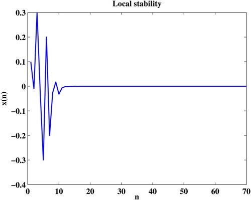
Example 1.

Figure 1 depicts the local asymptotic behaviour of the solutions around the equilibrium. The values of the constants are successfully selected by $c_1=0.2,c_2=1,c_3=2,c_4=3,x_{-6}=-0.2,x_{-5}=0.2,x_{-4}=-0.3,x_{-3}=-0.02,x_{-2}=-0.3,x_{-1}=-0.01,x_0=\mathrm{0.1.}$

Figure 1. Local asymptotic behaviour.

Example 2.

This example is allocated to show the global nature of the solutions under the values $c_1=0.3,c_2=2,c_3=0.5,c_4=5,x_{-6}=-1,x_{-5}=2,x_{-4}=-5,x_{-3}=3,x_{-2}=6,x_{-1}=-7,x_0=8.$ See Figure 2.

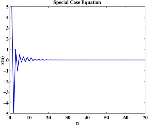
Example 4.

We plot in Figure 3 the behaviour of Equation (11)(11) $$x_{n+1}=x_{n-1}-\frac{x_{n-1}{x}_{n-4}}{x_{n-4}+x_{n-6},},$$(11) under some random initial conditions which are $x_{-6}=0.3,x_{-5}=-0.2,x_{-4}=0.5,x_{-3}=-1,x_{-2}=1,x_{-1}=-5,x_0=5.$

6. Conclusion

In brief, we have shown the stability of Equation (2)(2) $$x_{n+1}=c_1{x}_{n-1}-\frac{c_2{x}_{n-1}{x}_{n-4}}{c_3{x}_{n-4}+c_4{x}_{n-6}},n=0,1,\dots ,$$(2) under some powerful and effective hypotheses. In particular, the local stability of the fixed point occurs if $c_2(c_4-c_3)<(1-c_1){(c_3+c_4)}^2,$ and the global behaviour of the equilibrium point takes place if $c_1<1,$ as can be observed in Figure 1 and Figure 2, respectively. Other conditions for the local and global stability are discovered and illustrated. In Section 4, the exact solution of Equation (11)(11) $$x_{n+1}=x_{n-1}-\frac{x_{n-1}{x}_{n-4}}{x_{n-4}+x_{n-6},},$$(11) has been perfectly determined using Fibonacci sequence.

Figure 2. Global nature about the equilibrium.

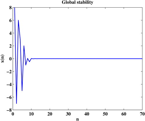
Figure 3. The behaviour of Equation (11)(11) $$x_{n+1}=x_{n-1}-\frac{x_{n-1}{x}_{n-4}}{x_{n-4}+x_{n-6},},$$(11) at $x_{-6}=0.3,x_{-5}=-0.2,x_{-4}=0.5,x_{-3}=-1,x_{-2}=1,x_{-1}=-5,x_0=5.$

Disclosure statement

No potential conflict of interest was reported by the author(s).

References

- Abdelrahman, M. A. E. (2019). On the difference equation zm+1=f(zm,zm−1,…,zm−k). Journal of Taibah University for Science, 13(1), 1014–1021. doi:10.1080/16583655.2019.1678866
- Abdelrahman, M. A. E., Chatzarakis, G. E., Tongxing, L., & Osama, M. (2018). On the difference equation xn+1=axn−l+bxn−k+f(xn−l,xn−k), Advances in Difference Equations, 431, 1–14. doi:10.1186/s13662-018-1880-8.
- Agarwal, R. P. (1992). Difference equations and inequalities: Theory, Methods and Applications. New York: Marcel Dekker.
- Almatrafi, M. B. (2019). Solutions structures for some systems of fractional difference equations. Open Journal of Mathematical Analysis, 3(1), 52–61. doi:10.30538/psrp-oma2019.0032
- Almatrafi, M. B., & Alzubaidi, M. M.. (2019). Analysis of the qualitative behaviour of an eighth-order fractional difference equation. Open Journal of Discrete Applied Mathematics, 2(1), 41–47. doi:10.30538/psrp-odam2019.0010
- Almatrafi, M. B., & Elsayed, E. M. (2018). Solutions and formulae for some systems of difference equations. MathLAB Journal, 1(3), 356–369.
- Almatrafi, M. B., Elsayed, E. M., & Alzahrani, F. (2018). Qualitative behavior of two rational difference equations. Fundamental Journal of Mathematics and Applications, 1(2), 194–204. doi:10.33401/fujma.454999
- Almatrafi, M. B., Elsayed, E. M., & Alzahrani, F. (2019). Qualitative behavior of a quadratic second-order rational difference equation. International Journal of Advances in Mathematics, 2019(1), 1–14.
- Amleh, A. M., Grove, E. A., Georgiou, D. A., & Ladas, G. (1999). On the recursive sequencexn+1=α+xn−1/xn,. Journal of Mathematical Analysis and Applications, 233(2), 790–798. doi:10.1006/jmaa.1999.6346
- Belhannache, F., Touafek, N., & Abo-Zeid, R. (2016). On a higher-order rational difference equation. Journal of Applied Mathematics & Informatics, 34(5-6), 369–382. doi:10.14317/jami.2016.369
- Elabbasy, E.M., El-Metawally, H., & Elsayed, E.M. (2008). On the difference equation xn+1=axn−(bxn)/(cxn−dxn−1),. Advances in Difference Equations, 4(17), 1–10. doi:10.1155/ADE/2006/82579
- El-Moneam, M. A., & Zayed, E. M. E. (2014). Dynamics of the rational difference equation. Information Sciences Letters, 3(2), 45–53. doi:10.12785/isl/030202
- Elsayed, E. M. (2010). Dynamics of recursive sequence of order two. Kyungpook Mathematical Journal, 50(4), 483–497. doi:10.5666/KMJ.2010.50.4.483
- Fisher, M. E. (1984). Stability of a class of delay-difference equations. Nonlinear Analysis, Theory, Methods and Applications, 8(6), 645–654. doi:10.1016/0362-546X(84)90009-9
- Garić-Demirović, M., Nurkanović, M., & Nurkanović, Z. (2017). Stability, periodicity and Neimark-Sacker bifurcation of certain homogeneous fractional difference equations. International Journal of Difference Equations, 12(1), 27–53.
- Hamza, A. E. (2006). On the recursive sequence xn+1=α+xn−1/xn,. Journal of Mathematical Analysis and Applications., 322, 668–674.
- Khaliq, A., & Hassan, S.S. (2018). Dynamics of a rational difference equation xn+1=axn+(α+βxn−k)/(A+Bxn−k),. International Journal of Advances in Mathematics, 159–179. 2018 (1)
- Khyat, T., & Kulenović, M. R. S. (2017). The invariant curve caused by Neimark-Sacker bifurcation of a perturbed Beverton-Holt difference equation. International Journal of Difference Equations, 12(2), 267–280.
- Kocic, V. L., & Ladas, G. (1993). Global behavior of nonlinear difference equations of higher order with applications. Dordrecht: Kluwer Academic.
- Kostrov, Y., & Kudlak, Z. (2016). On a second-order rational difference equation with a quadratic term. International Journal of Difference Equations, 11(2), 179–202.
- Liu, K., Li, P., Han, F., & Zhong, W. (2018). Global dynamics of nonlinear difference equation xn+1=A+xn/xn−1xn−2. Journal of Computational Analysis and Applications, 24(6), 1125–1132.
- Moaaz, O., Chalishajar, D., & Bazighifan, O. (2019). Some qualitative behavior of solutions of general class of difference equations. Mathematics, 7(7), 585. doi:10.3390/math7070585
- Moranjkić, S., & Nurkanović, Z. (2017). Local and global dynamics of certain second-order rational difference equations containing quadratic terms. Advances in Dynamical Systems and Applications, 12(2), 123–157.
- Saleh, M., & Aloqeili, M. (2005). On the rational difference equation yn+1=A+yn−kyn. Applied Mathematics and Computation 171(1), 862–869.
- Simsek, D., Cinar, C., & Yalcinkaya, I. (2006). On the recursive sequence xn+1=xn−31+xn−1. International Journal of Contemporary Mathematical Sciences, 1, 475–480. doi:10.12988/ijcms.2006.06052