Boundary-domain integral method and homotopy analysis method for systems of nonlinear boundary value problems in environmental engineering

Abstract

In this paper we present the development of numerical methods for two problems in chemical engineering: adsorption of carbon dioxide into phenyl glycidyl ether and diffusion and reaction processes in a porous catalyst. Both problems are modelled by systems of two coupled nonlinear ordinary differential equations. Dirichlet and Neumann type boundary conditions are considered. We develop the standard homotopy analysis method and the boundary-domain element method to solve for the unknown steady-state concentrations of reactants. The validity of the proposed methods is checked and demonstrated by numerical examples. Convergence rates are compared and the advantages and drawbacks of the proposed methods are discussed and compared to the Mathematica NDSOLVE solver. We show, that the proposed homotopy analysis method features exponential convergence rate and is highly accurate and efficient. As low as 6 terms are needed to reach error norms of ${10}^{-5}.$ Furthermore, the boundary-domain integral approach is also capable of solving the same problem very efficiently, using a very coarse computational mesh (21 nodes).

KEYWRODS:

• Diffusion
• adsorption
• boundary-domain integral method
• homotopy analysis method
• environmental engineering

1. Introduction

Numerical experiments and simulations (AbdAlmjeed, 2017; Aswhad, 2011) are frequently used to model natural and engineering phenomena in the fields of physics, chemistry, biology and environmental sciences. The phenomena are usually modelled by a system of equations with appropriate boundary and initial conditions. One encounters ordinary or partial differential equations, which may be linear or nonlinear. Unfortunately, most of these equations do not have an analytical solution or closed form, which could be represented by well-known elementary functions. Therefore, there is always a demand to develop reliable and efficient mathematical methods to obtain either a numerical or an approximate solution of these problems.

Carbon dioxide is one of the most important gases in nature (Subramaniam, Krishnaperumal, & Lakshmanan, 2012) as it is used in photosynthesis. Furthermore, several engineering systems also make use of carbon dioxide, such as for extinguishing fires, for powering of pneumatic systems, for the production of carbonated soft drinks and to remove caffeine from coffee, precipitation processes (Choe, Oh, Kim, & Park, 2010; Park, Park, Kim, Park, & Oh, 2004; Subramaniam et al., 2012; Zhao, Han, Jakobsson, Louhi-Kultanen, & Alopaeus, 2016). Ever since excess carbon dioxide has been found to cause global warming, its chemical fixation is an important research area in the field of environmental engineering (Chatterjee, Rayalu, Kolev, & Krupadam, 2016).

We model the adsorption of carbon dioxide (CO₂) into phenyl glycidyl ether (PGE) by relating the concentrations of both species using a system of two coupled nonlinear ordinary differential equations. This process has been studied by Park et al. (2004) and Choe, Oh, et al. (2010). The approximate analytical expression for the steady-state concentrations of carbon dioxide and phenyl glycidyl ether have been presented by Subramaniam et al. (2012) using the Adomian’s decomposition method (ADM). The drawback of this approach is the need to calculate the Adomian polynomials, which is computationally demanding. The methods proposed in this paper, do not have such a drawback.

The Lane-Emden equation is used to model many phenomena in astrophysics and mathematical physics. The description of diffusion and reaction processes in a porous catalyst, which we consider in this paper, is one of them. Other examples include: the thermal behaviour of a spherical cloud of gas, the theory of stellar structure and the theory of thermionic currents. The systems of Lane-Emden equations arise when modelling many other physical phenomena as well (Khojasteh Salkuyeh & Tavakoli, 2016; Sun, Liu, & Keith, 2004; Wazwaz, 2001; Wazwaz & Rach, 2011). Wazwaz et al. ( Wazwaz, Rach, & Duan, 2013; Wazwaz, Rach, & Duan, 2014) used the Adomian decomposition method for solving the Volterra integral form of the Lane-Emden equations with initial values and boundary conditions.

Homotopy analysis method was developed by Liao (1992) and Liao (2003). Following that, the application of this method was widespread. It was successfully used to solve many linear and nonlinear equations and problems, for example: simulation of nonlinear water waves (Tao, Song, & Chakrabarti, 2007), nonlinear heat transfer (Abbasbandy, 2006; 2007; Rashidi et al., 2014; Sajid & Hayat, 2008),differential-difference equation (Wang, Zou, & Zhang, 2007), solving cubic and coupled nonlinear Schrödinger equations (Hassan & El-Tawil, 2011) and many others (Akram & Sadaf, 2017; Alamri, Ellahi, Shehzad, & Zeeshan, 2019; Ellahi, 2013; Khan, Bukhari, Marin, & Ellahi, 2019; Kumar & Kumar, 2014; Prakash, Tripathi, Triwari, Sait, & Ellahi, 2019; Riaz, Ellahi, Bhatti, & Marin, 2019; Zeeshan, Shehzad, Abbas, & Ellahi, 2019). These successful applications affirmed the authenticity, flexibility and effectiveness of HAM.

The main advantage of the standard HAM is that in most cases its solution series converges very rapidly. Typically, only few iterations lead to a very accurate solution. HAM is a universal method and can be used to solve different types of nonlinear equations. Due to homotopy, HAM gives great freedom in the selection of initial approximations and auxiliary linear operators. The original HAM has been upgraded by introducing an auxiliary parameter h, which enables control of the convergence of the series. With this modification, the HAM is more efficient than the ADM (Adomian, 1994).

The domain-decomposition based boundary-domain integral method (BDIM) has been successfully used to solve various fluid flow and heat transfer problems (Ravnik, Škerget, & Žunič, 2008; Ravnik, Skerget, & Zunic, 2009). It is based on the boundary element method (Haghighat & Binesh, 2014). In this work, we rework the method for the solution of two chemical engineering problems as an alternative to the homotopy analysis method. The proposed method is second order accurate and can, due to the inclusion of function derivatives into the system of equations, be a good alternative for problems, which feature sharp function profiles and large gradients.

In this work, HAM and BDIM are developed for the solution of two chemical engineering problems. Both methods are derived and adapted to work for the two chosen chemical engineering problems. The advantage of the proposed HAM method in this paper is that it features exponential convergence rate and it is not hindered by the nonlinearity of the problem, which is the case with the Adomian decomposition method, which was proposed by other authors. In the HAM method proposed in this paper, there is no need for calculation of the Adomian polynomials. Additionally, we present the boundary-domain integral approach and show that it is also capable of solving the same problem very efficiently, using a very coarse computational meshes.

The paper is organized as follows. The governing equations describing the chemical processes are presented in section 2. Boundary element based solution is shown in section 3. Homotopy analysis method is developed in section 4. Simulations and discussion is given in section 5, which is followed by conclusions in section 6.

2. Considered problems

2.1. Diffusion and reaction processes in porous catalyst

Diffusion and reaction processes in porous catalyst have been a topic of research of several authors. Sun et al. (2004) consider a planar nonlinear model of diffusion and reaction in porous catalysts using a decomposition method. Similarly, a spherical pellet is considered by Shi-Bin, Yan-Ping, and Scott (2003). Rach, Duan, and Wazwaz (2014) proposed the Adomian decomposition method for the solution of the catalytic diffusion reactions.

Considering mass balance on a differential volume element in a spherical porous medium we may write the following transient diffusion-reaction equation (Bird, Stewart, & Lightfoot, 2007) (1) $$\frac{\partial c\prime }{\partial t}=\nabla ·D\nabla c\prime -R,$$(1) where c is the reactant concentration, t is time, D the effective diffusivity of the reactant and R is the rate of reaction per unit volume. We assume that the process is steady state and that the diffusivity is constant (temperature variations are small), thus we may simplify (2) $$D{\nabla }^{2}c\prime =R,$$(2)

Let r measure the distance from the centre of the catalyst pellet ($r\prime =0$) to the surface ($r\prime =r_0$). The process is subjected to the following boundary conditions (3) $${\frac{\partial c\prime }{\partial r\prime }|}_{r\prime =0}=0,\mathrm{\hspace{1em}}\mathrm{\hspace{1em}}c\prime (r_0)=c_0$$(3) where c_s is the reactant concentration at the surface of the porous medium. Now we consider a n – th order irreversible reaction and model the reaction term using power-law kinetics as $R=k_{v}c{\prime }^n,$ where the reaction constant is k_v and it is in general temperature dependent.

Introducing nondimenzionaliton $r=r\prime /r_0$ and $c=c\prime /c_0$ and considering spherical symmetry we get (4) $$\frac{d{c}^2}{d{r}^2}+\frac{2}{r}\frac{dc}{dr}={\varphi }^2{c}^n,\mathrm{\hspace{1em}}\mathrm{\hspace{1em}}{\frac{dc}{dr}|}_{r=0}=0,\mathrm{\hspace{1em}}\mathrm{\hspace{1em}}c(1)=1$$(4) where $\varphi$ is the Thiele modulus ${\varphi }^2=r_0^{2}k{c}_0^{n-1}/D.$ The derivation of the above expression is based on the validity of Fick’s law, i.e., concentration independent diffusivity.

In multicomponent mixture the transport of species must be described by Maxwell-Stefan equations. The application of these to mass transport in porous medium leads to the Dusty Fluid Model (Higler, Krishna, & Taylor, 2000). Applying these, we obtain the following catalyst diffusion model (Flockerzi & Sundmacher, 2011) (5) $$\frac{d{c}^2}{d{r}^2}+\frac{2}{r}\frac{dc}{dr}=\frac{N}{D}R,$$(5) where D is a constant matrix of diffusion coefficients, N is the stoichiometry matrix of the considered reaction network and R is a vector of reaction kinetics expressions. Since chemical reactions are mostly based on nono-molecular or bi-molecular events, the rate expressions are linear, bilinear or quadratic expressions. For this kind of reaction kinetics, we can identify a sub-vector u containing concentrations of species which appear in linear and bilinear forms and another vector v containing concentrations of species which also appear in quadratic terms. An example of such a case is acid-catalysed dimerization of C4-olefines (Talwalkar et al., 2007). This class of catalyst diffusion problems can be reformulated as a 2 D Lane-Emden boundary value problem (Flockerzi & Sundmacher, 2011): (6) $$\frac{d^{2}u}{d{r}^2}+\frac{2}{r}\frac{du}{dr}=k_{11}{u}^2+k_{12}uv$$(6) (7) $$\frac{d^{2}v}{d{r}^2}+\frac{2}{r}\frac{dv}{dr}=k_{21}{u}^2+k_{22}uv$$(7) in the domain $r\in [0,1]$ having the following boundary conditions (8) $${\frac{du}{dr}|}_{r=0}=0,\hspace{1em}u(1)={\beta }_1,\hspace{1em}{\frac{dv}{dr}|}_{r=0}=0,\hspace{1em}v(1)={\beta }_2.$$(8)

Here, β₁ and β₂ are positive constants and k is a nonzero matrix.

2.2. Absorption of carbon dioxide into phenyl glycidyl ether

Due to global warming, chemical fixation of carbon dioxide has become an important research topic and adsorption is on the processes capable to address this issue. The problem of absorption of carbon dioxide into phenyl glycidyl ether has been investigated by several authors. Choe, Oh, et al. (2010) experimentally studied absorption of carbon dioxide with the aid of a catalyst. (Duan, Rach, & Wazwaz, 2015; Duan & Rach, 2011) proposed the use of Adomian decomposition method for the simulation of the absorption of carbon dioxide into phenyl glycidyl ether. Theoretical analysis of mass transfer was given by Subramaniam et al. (2012).

The reaction consists of two consecutive steps: a reversible reaction between PGE and a catalyst THA-CP-MS41 (QX) to form an intermediate complex C₁ and a reaction between the complex and carbon dioxide to form the catalyst and a five-membered cyclic carbonate C. The reactions are (9) $$B+QX{\leftrightarrow }_{k_2}^{k_1}{C}_1$$(9) (10) $$A+C_1{\to }_{k_3}C+QX$$(10) k₁, k₂ and k₃ are reaction rates. Governing equations (Bird et al., 2007) for mass balances of CO₂ and PGE obtained using film theory are (Choe, Oh, et al., 2010): (11) $$r_{A,\mathit{cons}}=\frac{c_B{S}_t}{\frac{1}{k_1}+\frac{1}{K_1{k}_3{c}_a}+\frac{c_B}{k_3{c}_A}},\hspace{1em}{D}_A\frac{d^2{c}_A}{d{z}^2}=r_{A,\mathit{cons}},\hspace{1em}{D}_B\frac{d^2{c}_B}{d{z}^2}=r_{A,\mathit{cons}},$$(11) where S_t is the area of the catalyst, c_A and c_B are concentrations of CO₂ and PGE, K₁ is the reaction equilibrium constant, D_A and D_B are diffusivity of CO₂ and PGE, $r_{A,\mathit{cons}}$ is the steady state CO₂ chemical reaction rate and z is the distance. The boundary conditions are: $c_A(z=0)=c_{A0},d{c}_B/dz(z=0)=0,c_A(z=L)=c_{AL},c_B(z=L)=c_{BL}.$ These equations may be normalized and rewritten in terms of the non-dimensional distance $r=z/L:$ (12) $$\frac{d^{2}u}{d{r}^2}=\frac{a_{1}uv}{1+b_{1}u+b_{2}v}$$(12) (13) $$\frac{d^{2}v}{d{r}^2}=\frac{a_{2}uv}{1+b_{1}u+b_{2}v}$$(13) with boundary conditions: (14) $$u(0)=1,\mathrm{\hspace{1em}}\mathrm{\hspace{1em}}u(1)=k,\mathrm{\hspace{1em}}\mathrm{\hspace{1em}}{\frac{dv}{dr}|}_{r=0}=0,\mathrm{\hspace{1em}}\mathrm{\hspace{1em}}v(1)=1.$$(14)

The a₁, a₂, b₁ and b₂ are normalized parameters and u and v are dimensionless concentrations of CO₂ and PGE. The ratio between CO₂ concentrations at both sides of the domain is $k=c_{A0}/c_{AL}.$

3. Solution by boundary-domain integral method

Due to the diffusive nature of the considered transport processes, both boundary value problems, defined by Equations (6)–(8) and (12)–(14) feature a second order derivative, which describes diffusion at constant diffusivity. Mixed Dirichlet/Neumann boundary conditions are known for both cases. For a general 3 D setting, all equations may be written as (15) $${\nabla }^{2}u=f,$$(15) where u is the unknown function and f is a nonlinear forcing term. We consider Dirichlet and/or Neumann type boundary conditions (16) $$\begin{array}{l}\Gamma =\partial \Omega ={\Gamma }_D\cup {\Gamma }_N,\\ u(\mathbf{r})=\overline{u}(\mathbf{r}),\mathrm{\hspace{1em}}\mathrm{\hspace{1em}}\mathbf{r}\in {\Gamma }_D,\\ \mathbf{n}·\nabla u(\mathbf{r})=q(\mathbf{r})=\overline{q}(\mathbf{r}),\mathrm{\hspace{1em}}\mathrm{\hspace{1em}}\mathbf{r}\in {\Gamma }_N,\end{array}$$(16) where Γ_D is the Dirichlet part of the boundary and Γ_N is the Neumann part. At the Neumann part of the boundary the flux $q(\mathbf{r})$ is known and set to a known value of $\overline{q}(\mathbf{r}).$ At the Dirichlet part of the boundary, the function $u(\mathbf{r})$ is set to a known value of $\overline{u}(\mathbf{r}).$ Using a source point $\mathrm{\xi }\in \Gamma$ at the boundary we can recast the Poisson type equation (15)(15) $${\nabla }^{2}u=f,$$(15) into its integral representation (Wrobel, 2002): (17) $$c(\mathrm{\xi })u(\mathrm{\xi })+{\int }_{\Gamma }u\nabla u^{\star }·d\Gamma ={\int }_{\Gamma }{u}^{\star }\nabla u·d\Gamma +{\int }_{\Omega }{u}^{\star }fd\Omega ,$$(17) where $u^{\star }(\mathbf{r},\mathrm{\xi })=1/4\pi |\mathbf{r}-\mathrm{\xi }|$ is the fundamental solution for the diffusion operator, The free coefficient $c(\mathrm{\xi })$ is determined using solid surface angle at the source point position. The domain integral term in Equation (17)(17) $$c(\mathrm{\xi })u(\mathrm{\xi })+{\int }_{\Gamma }u\nabla u^{\star }·d\Gamma ={\int }_{\Gamma }{u}^{\star }\nabla u·d\Gamma +{\int }_{\Omega }{u}^{\star }fd\Omega ,$$(17) results from the source term on the right hand side of Equation (15)(15) $${\nabla }^{2}u=f,$$(15) .

In order to write a discrete version of Equation (17)(17) $$c(\mathrm{\xi })u(\mathrm{\xi })+{\int }_{\Gamma }u\nabla u^{\star }·d\Gamma ={\int }_{\Gamma }{u}^{\star }\nabla u·d\Gamma +{\int }_{\Omega }{u}^{\star }fd\Omega ,$$(17) we must interpolate the unknown function and its flux over boundary and domain elements. We employ 27 noded hexahedral domain elements, which enable quadratic interpolation of function in the domain using shape functions ${\Phi }_i.$ Flux is interpolated on the boundary only. We use four noded discontinuous linear interpolation functions ${\varphi }_i.$ Interpolation of function at boundary elements is performed using nine nodes and quadratic shape functions ${\phi }_i.$ Finally, the discrete version of Equation (17)(17) $$c(\mathrm{\xi })u(\mathrm{\xi })+{\int }_{\Gamma }u\nabla u^{\star }·d\Gamma ={\int }_{\Gamma }{u}^{\star }\nabla u·d\Gamma +{\int }_{\Omega }{u}^{\star }fd\Omega ,$$(17) is (18) $$\begin{array}{c}c(\mathrm{\xi })u(\mathrm{\xi })+\sum _b\sum _i{\alpha }_{b,i}{u}_{b,i}{\int }_{{\Gamma }_b}{\phi }_i\nabla u^{\star }·d\Gamma =\sum _b\sum _i{\alpha }_{b,i}{q}_{b,i}{\int }_{{\Gamma }_b}{\varphi }_i{u}^{\star }d\Gamma \\ +\sum _e\sum _i{f}_{e,i}{\int }_{{\Omega }_e}{\Phi }_i{u}^{\star }d\Omega ,\end{array}$$(18) where b lists boundary elements, e domain elements and i shape functions. The integrals of Equation (18)(18) $$\begin{array}{c}c(\mathrm{\xi })u(\mathrm{\xi })+\sum _b\sum _i{\alpha }_{b,i}{u}_{b,i}{\int }_{{\Gamma }_b}{\phi }_i\nabla u^{\star }·d\Gamma =\sum _b\sum _i{\alpha }_{b,i}{q}_{b,i}{\int }_{{\Gamma }_b}{\varphi }_i{u}^{\star }d\Gamma \\ +\sum _e\sum _i{f}_{e,i}{\int }_{{\Omega }_e}{\Phi }_i{u}^{\star }d\Omega ,\end{array}$$(18) depend solely on the mesh geometry and source point location. They are calculated in advance and reused during the iterative solution process. The Gaussian quadrature algorithm is used to calculate the integrals. We use indirect calculation of $c(\mathrm{\xi })$ using a known solution of the rigid body movement. The accuracy of integration is checked using nodes with known value of $c(\mathrm{\xi }).$

A collocation scheme is used to write a system of linear equations for the unknown values of function and flux. The source point $\mathrm{\xi }$ is placed into boundary nodes and the following matrices of integrals are thus calculated: (19) $$\left[H\right]={\int }_{\Gamma }{\phi }_i\nabla u^{\star }·\mathbf{n}d\Gamma ,\hspace{1em}\left[G\right]={\int }_{\Gamma }{\varphi }_i{u}^{\star }d\Gamma ,\hspace{1em}\left[B\right]={\int }_{\Omega }{\Phi }_i{u}^{\star }d\Omega .$$(19)

Let the square brackets denote matrices and curly brackets vectors of nodal values of functions. Using this notation the discrete version of Equation (18)(18) $$\begin{array}{c}c(\mathrm{\xi })u(\mathrm{\xi })+\sum _b\sum _i{\alpha }_{b,i}{u}_{b,i}{\int }_{{\Gamma }_b}{\phi }_i\nabla u^{\star }·d\Gamma =\sum _b\sum _i{\alpha }_{b,i}{q}_{b,i}{\int }_{{\Gamma }_b}{\varphi }_i{u}^{\star }d\Gamma \\ +\sum _e\sum _i{f}_{e,i}{\int }_{{\Omega }_e}{\Phi }_i{u}^{\star }d\Omega ,\end{array}$$(18) is (20) $$\left[H\right]\left\{u\right\}=\left[G\right]\left\{q\right\}+\left[B\right]\left\{f\right\}.$$(20)

As the boundary-domain integral method requires discretization of the domain and since the matrix of domain integrals $[B]$ is full, we avoid excessive storage and computational time usage by using a domain decomposition technique (Ramšak, Škerget, Hriberšek, & Žunič, 2005) Domain decomposition leads to a sparse system of equations. In this work, we consider the subdomains to be domain mesh elements. Connection between subdomains is obtained by considering that the function and the flux must be continuous across subdomains boundaries. The described procedure leads to a sparse and over-determined system of linear equations. We use (Paige & Saunders, 1982) least-squares solver with diagonal preconditioning to find the solution.

As the problems considered in this paper are nonlinear (the forcing function f in Eq. (15)(15) $${\nabla }^{2}u=f,$$(15) depends on u), we set up an iteration procedure during which, we estimate f using values of u in the previous iteration. Underrelaxation of 0.1 was used to achieve convergence. Furthermore, as the problems considered are 1 D and the BDIM method is written in 3 D, we used appropriate (zero flux) boundary conditions on the side walls.

4. Solution by homotopy analysis method

To verify the basic idea of HAM for a nonlinear system of ordinary differential equations (Bataineh, Noorani, & Hashim, 2009; Gabriel, 2016; Liao, 2004; Wazwaz, 2009), let us consider this problem: (21) $$N_i[u_i(x)]=0,i=1,2,\dots ,n$$(21) where N_i are the nonlinear operators, x is the independent variable and $u_i(x)$ are the unknown functions. To clarify this method simplify, we will ignore the conditions. Liao (2004) and Wazwaz (2009) configured the so-called zeroth-order deformation equation (22) $$(1-q)L[{\theta }_i(x;q)-u_{i,0}(x)]=q{h}_i\left\{N_i\right[{\theta }_i(x;q)\left]\right\}$$(22) where $q\in [0,1]$ represents an embedding parameter, h_i represent the nonzero auxiliary functions, L is the auxiliary linear operator, $u_{i,0}(x)$ represent the initial guesses of the function $u_i(x)$ and ${\theta }_i(x;q)$ are unknown functions. The advantage of HAM is that there is great freedom in the selection of the auxiliary objects, by means of h_i and L.

It is obvious that when putting the parameter q = 0 and q = 1, Equation (22)(22) $$(1-q)L[{\theta }_i(x;q)-u_{i,0}(x)]=q{h}_i\left\{N_i\right[{\theta }_i(x;q)\left]\right\}$$(22) will become (23) $${\theta }_i(x;0)=u_{i,0}(x)\mathrm{\hspace{1em}}\mathrm{\hspace{1em}}\text{and}\mathrm{\hspace{1em}}\mathrm{\hspace{1em}}{\theta }_i(x;1)=u_i(x),$$(23) respectively. Therefore, when q increases from 0 to 1, the solution ${\theta }_i(x;q)$ will vary from the initial guess $u_{i,0}(x)$ to the solution $u_i(x).$ The expansion of ${\theta }_i(x;q)$ in Taylor series with respect to q will be: (24) $${\theta }_i(x;q)=u_{i,0}(x)+\sum _{m=1}^{+\infty }{u}_{i,m}(x)q^m,$$(24) where (25) $$u_{i,m}=\frac{1}{m!}{\frac{{\partial }^m{\theta }_i(x;q)}{\partial q^m}|}_{(q=0)}.$$(25)

The auxiliary parameters h_i are the important to ensure the convergence of the series (Liao, 1992). So, if the auxiliary parameters h_i, the auxiliary linear operator and the initial guesses $u_{i,0}(x),$ are appropriately chosen, then the series (Liao, 1992) will converge at q = 1. Thus (26) $${\theta }_i(x;1)=u_{i,0}(x)+\sum _{m=1}^{+\infty }{u}_{i,m}(x),$$(26) must be one of the original nonlinear equation’s solutions, which is proved by Liao (2004) and Wazwaz (2009). If $h_i=-1,$ then (Khojasteh Salkuyeh & Tavakoli, 2016) will become (27) $$(1-q)L[{\theta }_i(x;q)-u_{i,0}(x)]+q\left\{N_i\right[{\theta }_i(x;q)\left]\right\}=0,$$(27)

This zeroth-order deformation equation is used in the homotopy perturbation method (HPM) [Rach et al., 2014). In accordance with the relationship (Liao, 2003), the governing equation could be derived from the zeroth-order deformation equation (22)(22) $$(1-q)L[{\theta }_i(x;q)-u_{i,0}(x)]=q{h}_i\left\{N_i\right[{\theta }_i(x;q)\left]\right\}$$(22) .

Let us define a vector (28) $${\overrightarrow{u}}_{i,n}(x)=\{u_{i,0}(x),u_{i,1}(x),u_{i,2}(x),u_{i,n}(x)\},i=1,2,,n.$$(28)

By differentiating equation (27)(27) $$(1-q)L[{\theta }_i(x;q)-u_{i,0}(x)]+q\left\{N_i\right[{\theta }_i(x;q)\left]\right\}=0,$$(27) with respect to the embedding parameter q for m times, then substituting q = 0 and dividing them by $m!,$ the mth-order deformation equation is derived as: (29) $$L[u_{i,m}(x)-X_m{u}_{i,m-1}(x)]=h_i{R}_{i,m}({\overrightarrow{u}}_{i,m-1}),$$(29) where (30) $$R_{i,m}({\overrightarrow{u}}_{i,m-1})=\frac{1}{(m-1)!}{\frac{{\partial }^{m-1}{\theta }_i(x;q)}{\partial q^{m-1}}|}_{(q=0)}.$$(30) and (31) $$X_m=\{\begin{array}{c}0\text{when}m\le 1,\hfill \\ 1\text{when}m>1.\hfill \end{array}$$(31)

Implementing $L^{-1}$ (an integral operator) on Equation (29)(29) $$L[u_{i,m}(x)-X_m{u}_{i,m-1}(x)]=h_i{R}_{i,m}({\overrightarrow{u}}_{i,m-1}),$$(29) in both sides, we have (32) $$u_{i,m}(x)=X_m{u}_{i,m-1}(x)+h{L}^{-1}[H(x)R_m(u_{i,m-1}^{\to })],$$(32) in iterative way, it is easy to get $u_{i,m}$ for $m\ge 1$ and for mth-order the following will be obtained (33) $$u(x)=\sum _{m=0}^j{u}_{i,m}(x),$$(33)

An accurate approximate function for the general differential equation (21)(21) $$N_i[u_i(x)]=0,i=1,2,\dots ,n$$(21) will be obtained when $j\to +\infty ,$ if Equation (21)(21) $$N_i[u_i(x)]=0,i=1,2,\dots ,n$$(21) possesses a unique solution, then the HAM will present this unique solution, but is Equation (21)(21) $$N_i[u_i(x)]=0,i=1,2,\dots ,n$$(21) hasn’t a unique solution then this method will provide a solution among another active solutions. In the following, each problem will be reviewed, and then we will apply the HAM on each of them.

4.1. The HAM for solving the Lane-Emden boundary value problem

The boundary value problem for the coupled equations of Lane-Emden with the product nonlinearities (Flockerzi & Sundmacher, 2011; Rach et al., 2014) are: (34) $$u″(x)+\frac{2}{x}u\prime (x)+f_1(u(x),v(x))=0,$$(34) (35) $$v″(x)+\frac{2}{x}v\prime (x)+f_2(u(x),v(x))=0,$$(35) (36) $$\begin{array}{c}{f}_1(u(x),v(x))=-k_{11}{u}^2(x)-k_{12}u(x)v(x),\\ f_2(u(x),v(x))=-k_{21}{u}^2(x)-k_{22}u(x)v(x),\end{array}$$(36) with the following boundary conditions $$u\prime (0)=0,\mathrm{\hspace{1em}}u(1)={\beta }_1,\mathrm{\hspace{1em}}v\prime (0)=0,\mathrm{\hspace{1em}}v(1)={\beta }_2.$$

The above boundary value problem represents a model of catalytic diffusion reactions (Flockerzi & Sundmacher, 2011). The parameters of the system: ${\beta }_1,{\beta }_2,k_{11},k_{12},k_{21}\text{and}{k}_{22}$ can be selected for the actual chemical reactions. Flockerzi and Sundmacher (2011) assumed that in the qualitative analysis for the solutions. In the following, we produce an approximate solution for the above nonlinear problem using the HAM (Bataineh et al., 2009; Gabriel, 2016; Liao, 2004; Wazwaz, 2009). In order to implement this method to the current system, we will solve the system introduced by Rach et al. (2014) which is used in the modified ADM. So, the system above will be reduced to the following form of two-coupled nonlinear Fredholm-Volterra integral equations (37) $$u(x)={\beta }_1+{\int }_0^{1}t(1-t)f_1(u(t),v(t))dt-{\int }_0^{x}t\left(1-\frac{t}{x}\right)f_1(u(t),v(t))dt,$$(37) (38) $$v(x)={\beta }_2+{\int }_0^{1}t(1-t)f_2(u(t),v(t))dt-{\int }_0^{x}t\left(1-\frac{t}{x}\right)f_2(u(t),v(t))dt,$$(38)

To implement the HAM to the nonlinear system above, the basic idea of HAM will be applied. So, the zeroth approximations are $$\begin{array}{c}{u}_0(x)={\beta }_1,\\ v_0(x)={\beta }_2.\end{array}$$

The linear operators for Equations (37)(37) $$u(x)={\beta }_1+{\int }_0^{1}t(1-t)f_1(u(t),v(t))dt-{\int }_0^{x}t\left(1-\frac{t}{x}\right)f_1(u(t),v(t))dt,$$(37) and (38)(38) $$v(x)={\beta }_2+{\int }_0^{1}t(1-t)f_2(u(t),v(t))dt-{\int }_0^{x}t\left(1-\frac{t}{x}\right)f_2(u(t),v(t))dt,$$(38) , respectively will be (39) $$L[{\theta }_i(x;q)]={\theta }_i(x;q),i=1,2.$$(39)

Now, defining a system of nonlinear operators in the following forms: (40) $$N_1[{\theta }_i(x;q)]={\theta }_1(x;q)-{\beta }_1-{\int }_0^{1}t(1-t)f_1({\theta }_1(t;q),{\theta }_2(t;q))dt+{\int }_0^{x}t\left(1-\frac{t}{x}\right)f_1({\theta }_1(t;q),{\theta }_2(t;q))dt,$$(40) (41) $$N_2[{\theta }_i(x;q)]={\theta }_2(x;q)-{\beta }_2-{\int }_0^{1}t(1-t)f_2({\theta }_1(t;q),{\theta }_2(t;q))dt+{\int }_0^{x}t\left(1-\frac{t}{x}\right)f_2({\theta }_1(t;q),{\theta }_2(t;q))dt,$$(41)

According to the basic idea of HAM, the mth-order deformation equations will be (42) $$L[u_m(x)]=X_m{u}_{m-1}(x)+h{R}_{1,m}({\overrightarrow{u}}_{m-1},{\overrightarrow{v}}_{m-1}),$$(42) (43) $$L[v_m(x)]=X_m{v}_{m-1}(x)+h{R}_{2,m}({\overrightarrow{u}}_{m-1},{\overrightarrow{v}}_{m-1}),$$(43) where, for $m\ge 1,$ we have (44) $$\begin{array}{c}{R}_{1,m}=u_{m-1}(x)-(1-X_m){\beta }_1-{\int }_0^{1}t(1-t)(-k_{11}(\sum _{j=0}^{m-1}{u}_j{u}_{m-1-j})-\\ k_{12}(\sum _{j=0}^{m-1}{u}_j{v}_{m-1-j}))dt+{\int }_0^{x}t(1-\frac{t}{x})(-k_{11}(\sum _{j=0}^{m-1}{u}_j{u}_{m-1-j})-k_{12}(\sum _{j=0}^{m-1}{u}_j{v}_{m-1-j}))dt,\end{array}$$(44) (45) $$\begin{array}{c}{R}_{2,m}=v_{m-1}(x)-(1-X_m){\beta }_2-{\int }_0^{1}t(1-t)(-k_{21}(\sum _{j=0}^{m-1}{u}_j{u}_{m-1-j})\\ -k_{22}(\sum _{j=0}^{m-1}{u}_j{v}_{m-1-j}))dt+{\int }_0^{x}t(1-\frac{t}{x})(-k_{21}(\sum _{j=0}^{m-1}{u}_j{u}_{m-1-j})-k_{22}(\sum _{j=0}^{m-1}{u}_j{v}_{m-1-j}))dt.\end{array}$$(45)

We get the following $$\begin{array}{l}{u}_0(x)={\beta }_1,\\ v_0(x)={\beta }_2,\\ u_1(x)=h\left(\frac{{\beta }_1{}^2{k}_{11}}{6}-\frac{1}{6}{\beta }_1{}^2{k}_{11}{x}^2+\frac{{\beta }_1{\beta }_2{k}_{12}}{6}-\frac{1}{6}{\beta }_1{\beta }_2{k}_{12}{x}^2\right),\\ v_1(x)=h\left(\frac{{\beta }_1{}^2{k}_{21}}{6}-\frac{1}{6}{\beta }_1{}^2{k}_{21}{x}^2+\frac{{\beta }_1{\beta }_2{k}_{22}}{6}-\frac{1}{6}{\beta }_1{\beta }_2{k}_{22}{x}^2\right),\end{array}$$ and so on. When h = − 1, we obtain $$\begin{array}{c}{u}_1(x)=-\frac{{\beta }_1{}^2{k}_{11}}{6}+\frac{1}{6}{\beta }_1{}^2{k}_{11}{x}^2-\frac{{\beta }_1{\beta }_2{k}_{12}}{6}+\frac{1}{6}{\beta }_1{\beta }_2{k}_{12}{x}^2,\\ v_1(x)=-\frac{{\beta }_1{}^2{k}_{21}}{6}+\frac{1}{6}{\beta }_1{}^2{k}_{21}{x}^2-\frac{{\beta }_1{\beta }_2{k}_{22}}{6}+\frac{1}{6}{\beta }_1{\beta }_2{k}_{22}{x}^2,\end{array}$$

Also, we get $$\begin{array}{c}{u}_2(x)=\frac{7{\beta }_1{}^3{k}_{11}{}^2}{180}+\frac{1}{60}{\beta }_1{}^3{k}_{11}{}^2{x}^4-\frac{1}{18}{\beta }_1{}^3{k}_{11}{}^2{x}^2+\frac{7}{120}{\beta }_1{}^2{\beta }_2{k}_{11}{k}_{12}+\frac{1}{40}{\beta }_1{}^2{\beta }_2{k}_{11}{k}_{12}{x}^4-\\ \frac{1}{12}{\beta }_1{}^2{\beta }_2{k}_{11}{k}_{12}{x}^2+\frac{7}{360}{\beta }_1{\beta }_2{}^2{k}_{12}{}^2+\frac{1}{120}{\beta }_1{\beta }_2{}^2{k}_{12}{}^2{x}^4-\frac{1}{36}{\beta }_1{\beta }_2{}^2{k}_{12}{}^2{x}^2+\frac{7}{360}{\beta }_1{}^3{k}_{12}{k}_{21}+\\ \frac{1}{120}{\beta }_1{}^3{k}_{12}{k}_{21}{x}^4-\frac{1}{36}{\beta }_1{}^3{k}_{12}{k}_{21}{x}^2+\frac{7}{360}{\beta }_1{}^2{\beta }_2{k}_{12}{k}_{22}+\frac{1}{120}{\beta }_1{}^2{\beta }_2{k}_{12}{k}_{22}{x}^4-\frac{1}{36}{\beta }_1{}^2{\beta }_2{k}_{12}{k}_{22}{x}^2\end{array}$$ $$\begin{array}{c}{v}_2(x)=\frac{7}{180}{\beta }_1{}^3{k}_{11}{k}_{21}+\frac{1}{60}{\beta }_1{}^3{k}_{11}{k}_{21}{x}^4-\frac{1}{18}{\beta }_1{}^3{k}_{11}{k}_{21}{x}^2+\frac{7}{360}{\beta }_1{}^2{\beta }_2{k}_{11}{k}_{22}+\frac{1}{120}{\beta }_1{}^2{\beta }_2{k}_{11}{k}_{22}{x}^4-\\ \frac{1}{36}{\beta }_1{}^2{\beta }_2{k}_{11}{k}_{22}{x}^2+\frac{7}{180}{\beta }_1{}^2{\beta }_2{k}_{12}{k}_{21}+\frac{1}{60}{\beta }_1{}^2{\beta }_2{k}_{12}{k}_{21}{x}^4-\frac{1}{18}{\beta }_1{}^2{\beta }_2{k}_{12}{k}_{21}{x}^2\\ +\frac{7}{360}{\beta }_1{\beta }_2{}^2{k}_{12}{k}_{22}+\frac{1}{120}{\beta }_1{\beta }_2{}^2{k}_{12}{k}_{22}{x}^4-\frac{1}{36}{\beta }_1{\beta }_2{}^2{k}_{12}{k}_{22}{x}^2+\frac{7}{360}{\beta }_1{}^3{k}_{21}{k}_{22}+\\ +\frac{1}{120}{\beta }_1{}^3{k}_{21}{k}_{22}{x}^4-\frac{1}{36}{\beta }_1{}^3{k}_{21}{k}_{22}{x}^2+\frac{7}{360}{\beta }_1{}^2{\beta }_2{k}_{22}{}^2+\frac{1}{120}{\beta }_1{}^2{\beta }_2{k}_{22}{}^2{x}^4-\frac{1}{36}{\beta }_1{}^2{\beta }_2{k}_{22}{}^2{x}^2\end{array}$$ and so on. Proceeding in this way, the components were also calculated but for brevity, they are not listed here.

The used approximate functions of solutions will be as in Rach et al. (2014), in the following formulas: (46) $$Y_{m+1}(x)=\sum _{n=0}^m{u}_n(x),Z_{m+1}(x)=\sum _{n=0}^m{v}_n(x),m\ge 0.$$(46)

The used convenient error remainder functions will be also as in Rach et al. (2014), in the forms (47) $$\begin{array}{c}E{R}_{1,n}(x)=\frac{d^2}{d{x}^2}{Y}_n(x)+\frac{2}{x}\frac{d}{dx}{Y}_n(x)+f_1(Y_n(x),Z_n(x)),\\ E{R}_{2,n}(x)=\frac{d^2}{d{x}^2}{Z}_n(x)+\frac{2}{x}\frac{d}{dx}{Z}_n(x)+f_2(Y_n(x),Z_n(x)),\end{array}$$(47) with the maximal error remainder parameters forms (48) $$ME{R}_{1,n}=\underset{{}_{0<x\le 1}}{\max }\left|E{R}_{1,n}(x)\right|,\mathrm{\hspace{1em}}ME{R}_{2,n}=\underset{{}_{0<x\le 1}}{\max }\left|E{R}_{2,n}(x)\right|,$$(48)

4.2. The HAM for solving the absorption of CO2 by the PGE boundary value problem

A model for steady state concentrations of carbon dioxide CO2 and PGE has been proposed as in Duan et al. (2015) and Subramaniam et al. (2012). The following system of two second order nonlinear ordinary differential equations representing the two chemicals must be solved: (49) $$u″(x)={\alpha }_{1}f(u(x),v(x)),$$(49) (50) $$v″(x)={\alpha }_{2}f(u(x),v(x)),$$(50) where (51) $$f=\frac{u(x)v(x)}{1+{\beta }_{1}u(x)+{\beta }_{2}v(x),}$$(51) with the following boundary conditions $u(0)=1,u(1)=k,v\prime (0)=0$ and $v(1)=1.$

Here u(x) stands for the CO2 concentration and v(x) is the PGE concentration. The normalized system parameters are ${\alpha }_1,{\alpha }_2,{\beta }_1$ and ${\beta }_2.$ The carbon dioxide concentration at catalyst surface is denoted by k Finally, the dimensionless distance from the centre is x (Duan et al., 2015).

Adomian (1994), Duan et al. (2015), Biazar, Babolian, and Islam (2004), have used the Adomian decomposition method to develop a solution of this problem. They transform the governing equations into a system of coupled integral equations. Due to the nonlinear nature of the problem, Adomian polynomials have to be calculated, which requires large computational resources.

In the following, we present an approximate solution of this nonlinear problem using the HAM (Bataineh et al., 2009; Gabriel, 2016; Liao, 2004; Wazwaz, 2009). In order to implement this method to the current system, we will solve the following system given in Flockerzi and Sundmacher (2011). So, (52) $$u(x)=1+(k-1)x-{\alpha }_{1}x{\int }_0^1{\int }_0^{x}f(u(t),v(t))\mathit{dtdt}+{\alpha }_1{\int }_0^x{\int }_0^{x}f(u(t),v(t))\mathit{dtdt},$$(52) (53) $$v(x)=1-{\alpha }_2{\int }_0^1{\int }_0^{x}f(u(t),v(t))\mathit{dtdt}+{\alpha }_2{\int }_0^x{\int }_0^{x}f(u(t),v(t))\mathit{dtdt},$$(53)

By implementing the HAM to the nonlinear system above, the selected zeroth approximations are (54) $$u_0(x)=1,$$(54) (55) $$v_0(x)=1,$$(55)

Consecutively we obtain the following terms by HAM: $$\begin{array}{l}{u}_1(x)=h\left(-(k-1)x-\frac{{\alpha }_1{x}^2}{2({\beta }_1+{\beta }_2+1)}+\frac{{\alpha }_{1}x}{2({\beta }_1+{\beta }_2+1)}\right)\\ v_1(x)=h\left(\frac{{\alpha }_2}{2({\beta }_1+{\beta }_2+1)}-\frac{{\alpha }_2{x}^2}{2({\beta }_1+{\beta }_2+1)}\right)\end{array}$$ and so on. When h = − 1, we get $$\begin{array}{c}{u}_1(x)=(-1+k)x-\frac{x{\alpha }_1}{2(1+{\beta }_1+{\beta }_2)}+\frac{x^2{\alpha }_1}{2(1+{\beta }_1+{\beta }_2)},\\ v_1(x)=-\frac{{\alpha }_2}{2(1+{\beta }_1+{\beta }_2)}+\frac{x^2{\alpha }_2}{2(1+{\beta }_1+{\beta }_2)},\end{array}$$

Also, we get $$\begin{array}{c}{u}_2(x)=\frac{{\alpha }_1{\beta }_2{}^{2}k{x}^3}{6{({\beta }_1+{\beta }_2+1)}^3}+\frac{{\alpha }_1{\beta }_{2}k{x}^3}{3{({\beta }_1+{\beta }_2+1)}^3}+\frac{{\alpha }_{1}k{x}^3}{6{({\beta }_1+{\beta }_2+1)}^3}+\frac{{\alpha }_1{\beta }_{1}k{x}^3}{6{({\beta }_1+{\beta }_2+1)}^3}+\frac{{\alpha }_1{\beta }_1{\beta }_{2}k{x}^3}{6{({\beta }_1+{\beta }_2+1)}^3}-\\ \frac{{\alpha }_1{\beta }_2{}^{2}kx}{6{({\beta }_1+{\beta }_2+1)}^3}-\frac{{\alpha }_1{\beta }_{2}kx}{3{({\beta }_1+{\beta }_2+1)}^3}-\frac{{\alpha }_{1}kx}{6{({\beta }_1+{\beta }_2+1)}^3}-\frac{{\alpha }_1{\beta }_{1}kx}{6{({\beta }_1+{\beta }_2+1)}^3}\\ -\frac{{\alpha }_1{\beta }_1{\beta }_{2}kx}{6{({\beta }_1+{\beta }_2+1)}^3}+\frac{{\alpha }_1{}^2{x}^4}{24{({\beta }_1+{\beta }_2+1)}^3}+\frac{{\alpha }_1{}^2{\beta }_2{x}^4}{24{({\beta }_1+{\beta }_2+1)}^3}+\frac{{\alpha }_1{\alpha }_2{x}^4}{24{({\beta }_1+{\beta }_2+1)}^3}\\ +\frac{{\alpha }_1{\alpha }_2{\beta }_1{x}^4}{24{({\beta }_1+{\beta }_2+1)}^3}-\frac{{\alpha }_1{}^2{x}^3}{12{({\beta }_1+{\beta }_2+1)}^3}-\frac{{\alpha }_1{}^2{\beta }_2{x}^3}{12{({\beta }_1+{\beta }_2+1)}^3}-\frac{{\alpha }_1{\beta }_2{}^2{x}^3}{6{({\beta }_1+{\beta }_2+1)}^3}\\ -\frac{{\alpha }_1{\beta }_2{x}^3}{3{({\beta }_1+{\beta }_2+1)}^3}-\frac{{\alpha }_1{x}^3}{6{({\beta }_1+{\beta }_2+1)}^3}-\frac{{\alpha }_1{\beta }_1{x}^3}{6{({\beta }_1+{\beta }_2+1)}^3}-\frac{{\alpha }_1{\beta }_1{\beta }_2{x}^3}{6{({\beta }_1+{\beta }_2+1)}^3}\\ -\frac{{\alpha }_1{\alpha }_2{x}^2}{4{({\beta }_1+{\beta }_2+1)}^3}-\frac{{\alpha }_1{\alpha }_2{\beta }_1{x}^2}{4{({\beta }_1+{\beta }_2+1)}^3}+\frac{{\alpha }_1{}^{2}x}{24{({\beta }_1+{\beta }_2+1)}^3}+\frac{{\alpha }_1{}^2{\beta }_{2}x}{24{({\beta }_1+{\beta }_2+1)}^3}\\ +\frac{5{\alpha }_1{\alpha }_{2}x}{24{({\beta }_1+{\beta }_2+1)}^3}+\frac{5{\alpha }_1{\alpha }_2{\beta }_{1}x}{24{({\beta }_1+{\beta }_2+1)}^3}+\frac{{\alpha }_1{\beta }_2{}^{2}x}{6{({\beta }_1+{\beta }_2+1)}^3}+\frac{{\alpha }_1{\beta }_{2}x}{3{({\beta }_1+{\beta }_2+1)}^3}\\ +\frac{{\alpha }_{1}x}{6{({\beta }_1+{\beta }_2+1)}^3}+\frac{{\alpha }_1{\beta }_{1}x}{6{({\beta }_1+{\beta }_2+1)}^3}+\frac{{\alpha }_1{\beta }_1{\beta }_{2}x}{6{({\beta }_1+{\beta }_2+1)}^3}\end{array}$$ $$\begin{array}{c}{v}_2(x)=\frac{{\alpha }_1{\alpha }_2}{24{({\beta }_1+{\beta }_2+1)}^3}+\frac{{\alpha }_1{\alpha }_2{\beta }_2}{24{({\beta }_1+{\beta }_2+1)}^3}+\frac{5{\alpha }_2{}^2}{24{({\beta }_1+{\beta }_2+1)}^3}+\frac{5{\alpha }_2{}^2{\beta }_1}{24{({\beta }_1+{\beta }_2+1)}^3}\\ +\frac{{\alpha }_2{\beta }_2{}^2}{6{({\beta }_1+{\beta }_2+1)}^3}+\frac{{\alpha }_2{\beta }_2}{3{({\beta }_1+{\beta }_2+1)}^3}+\frac{{\alpha }_2}{6{({\beta }_1+{\beta }_2+1)}^3}+\frac{{\alpha }_2{\beta }_1}{6{({\beta }_1+{\beta }_2+1)}^3}+\frac{{\alpha }_2{\beta }_1{\beta }_2}{6{({\beta }_1+{\beta }_2+1)}^3}-\\ -\frac{{\alpha }_2{\beta }_2{}^{2}k}{6{({\beta }_1+{\beta }_2+1)}^3}-\frac{{\alpha }_2{\beta }_{2}k}{3{({\beta }_1+{\beta }_2+1)}^3}-\frac{{\alpha }_{2}k}{6{({\beta }_1+{\beta }_2+1)}^3}-\frac{{\alpha }_2{\beta }_{1}k}{6{({\beta }_1+{\beta }_2+1)}^3}-\frac{{\alpha }_2{\beta }_1{\beta }_{2}k}{6{({\beta }_1+{\beta }_2+1)}^3}\\ +\frac{{\alpha }_2{\beta }_2{}^{2}k{x}^3}{6{({\beta }_1+{\beta }_2+1)}^3}+\frac{{\alpha }_2{\beta }_{2}k{x}^3}{3{({\beta }_1+{\beta }_2+1)}^3}+\frac{{\alpha }_{2}k{x}^3}{6{({\beta }_1+{\beta }_2+1)}^3}+\frac{{\alpha }_2{\beta }_{1}k{x}^3}{6{({\beta }_1+{\beta }_2+1)}^3}+\frac{{\alpha }_2{\beta }_1{\beta }_{2}k{x}^3}{6{({\beta }_1+{\beta }_2+1)}^3}+\\ +\frac{{\alpha }_1{\alpha }_2{x}^4}{24{({\beta }_1+{\beta }_2+1)}^3}+\frac{{\alpha }_1{\alpha }_2{\beta }_2{x}^4}{24{({\beta }_1+{\beta }_2+1)}^3}+\frac{{\alpha }_2{}^2{x}^4}{24{({\beta }_1+{\beta }_2+1)}^3}+\frac{{\alpha }_2{}^2{\beta }_1{x}^4}{24{({\beta }_1+{\beta }_2+1)}^3}-\frac{{\alpha }_1{\alpha }_2{x}^3}{12{({\beta }_1+{\beta }_2+1)}^3}\\ -\frac{{\alpha }_1{\alpha }_2{\beta }_2{x}^3}{12{({\beta }_1+{\beta }_2+1)}^3}-\frac{{\alpha }_2{\beta }_2{}^2{x}^3}{6{({\beta }_1+{\beta }_2+1)}^3}-\frac{{\alpha }_2{\beta }_2{x}^3}{3{({\beta }_1+{\beta }_2+1)}^3}-\frac{{\alpha }_2{x}^3}{6{({\beta }_1+{\beta }_2+1)}^3}\\ -\frac{{\alpha }_2{\beta }_1{x}^3}{6{({\beta }_1+{\beta }_2+1)}^3}-\frac{{\alpha }_2{\beta }_1{\beta }_2{x}^3}{6{({\beta }_1+{\beta }_2+1)}^3}-\frac{{\alpha }_2{}^2{x}^2}{4{({\beta }_1+{\beta }_2+1)}^3}-\frac{{\alpha }_2{}^2{\beta }_1{x}^2}{4{(\beta 1+{\beta }_2+1)}^3}\end{array}$$ and so on. Proceeding in this way, the components were also calculated but for brevity, they are not listed here.

The used approximate functions of solutions will be as in (Wazwaz, 2005). The used convenient error remainder functions will be also as in Duan et al. (2015), in the forms (56) $$\begin{array}{c}E{R}_{1,n}(x)=\frac{d^2}{d{x}^2}{Y}_n(x)-a_{1}f(Y_n(x),Z_n(x)),\\ E{R}_{2,n}(x)=\frac{d^2}{d{x}^2}{Z}_n(x)-a_{2}f(Y_n(x),Z_n(x)),\end{array}$$(56) and the maximal error remainder parameters are calculated as in equation (Wazwaz & Rach, 2011).

4.3. HAM convergence properties

4.3.1. Diffusion and reaction processes in porous catalyst

In order to validate the proposed HAM method and examine the HAM convergence properties, we solve the problem of diffusion and reaction processes in porous catalyst using the parameter values suggested by Wazwaz et al. (2014): ${\beta }_1=1,{\beta }_2=2,k_{11}=1,k_{12}=\frac{2}{5},k_{21}=\frac{1}{2},$ and $k_{22}=1.$ We will evaluate the approximate solutions, the error remainder and the maximal error remainder. 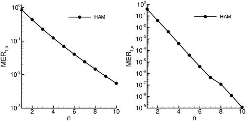Furthermore, $ME{R}_{1,n}$ and $ME{R}_{2,n}$ are calculated, so that the values of n are increasing from 1 to 10. In the left panel of Figure 1 we display the convergence curve for $ME{R}_{1,n}.$ The convergence of $ME{R}_{2,n}$ is similar.

Figure 1. Norms $ME{R}_{1,n}$ shown for HAM for $n=1,\dots ,10$ for the solution of the diffusion and reaction processes in porous catalyst problem (left) and the adsorption problem (right). Norms $ME{R}_{2,n}$ exhibit similar characteristics.

4.4. Absorption of carbon dioxide into phenyl glycidyl ether

In order to validate the proposed HAM method, we solve the problem of absorption of carbon dioxide into phenyl glycidyl ether using the parameter values suggested by Duan et al. (2015): ${\alpha }_1=1,{\alpha }_2=2,{\beta }_1=1,{\beta }_2=3$ and $k=0.5.$ We will evaluate the approximate solutions, the error remainder and the maximal error remainder. Furthermore, $ME{R}_{1,n}$ and $ME{R}_{2,n}$ are calculated, so that the values of n are increasing from 1 to 10. In the right panel of Figure 1 the convergence curve for $ME{R}_{1,n}.$ The convergence of $ME{R}_{2,n}$ is similar.

5. Simulations and discussion

5.1. Solution of the catalytic diffusion problem

In Figure 2 we compare concentration profiles for HAM and BDIM. The parameters used were: ${\beta }_1=1,$ ${\beta }_2=2,$ $k_{11}=1,$ $k_{12}=\frac{2}{5},$ $k_{21}=\frac{1}{2},$ $k_{22}=1.$

Figure 2. Comparison of solutions of the catalytic diffusion problem. u and v concentration profiles are presented for the HAM (left) and BDIM (right).

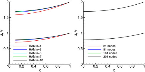
Looking at HAM results, we observe that solution obtained using $n\le 3$ are different from the accurate n = 10 solution, while for $n\ge 4$ the convergence profiles do not differ significantly. The BDIM results have been obtained using different computational grids. Grids having 21 to 201 equidistantly places nodes were used. Due to the simple nature of the problem (diffusion only) and due to the use of quadratic interpolation, we detect virtually no difference between results obtained on different meshes.

5.2. Solution of absorption of carbon dioxide into phenyl glycidyl ether

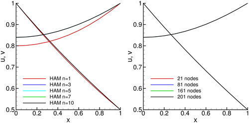
Solution profiles for the absorption of carbon dioxide into phenyl glycidyl ether are shown in Figure 3. The following parameters were used: $a_1=1,$ $a_2=2,$ $b_1=1,$ $b_2=3,$ $k=\mathrm{0.5.}$ In this case, only the n = 1 HAM solution show significant difference from the converged n = 10 solution, while all others ($n\ge 2$) are very close to each other. Similarly to the catalytic diffusion problem, the BDIM is able to capture the physics of the phenomena using a very coarse mesh (21 nodes).

Figure 3. Comparison of solutions of the absorption problem. u and v concentration profiles are presented for the HAM (left) and BDIM (right).

5.3. Comparison to Mathematica NDSOLVE solver

We solved both problems using Mathematica’s NDSOLVE functions. Please refer to the appendix for the complete code. In order to asses the difference in solutions, we calculated the RMS difference between solution profiles as (57) $$\mathit{RMS}(u)=\sqrt{\frac{\sum {(u-u_{\mathit{NDSOLVE}})}^2}{\sum {(u_{\mathit{NDSOLVE}})}^2}}$$(57)

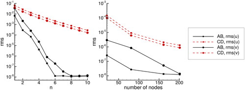
In Figure 4 we presented the RMS differences versus location x, while in Figure 5 average values are presented. We observe that the RMS error decreases with increasing n for the HAM method and with increasing number of nodes for the BDIM method. Looking at the RMS vs. x profile we see that the accuracy is approximately constant for all values of x. Accuracy of solution of the absorption problem is higher than the accuracy for the catalytic diffusion problem for both methods.

Figure 4. RMS difference between u and v concentration profiles and the Mathematica NDSLOVE solver. Results for the catalytic diffusion problem are shown in the top panels and results of absorption of carbon dioxide are shown in the bottom panels.

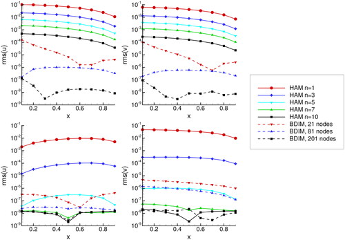
Figure 5. Average RMS difference between u and v concentration profiles and the Mathematica NDSLOVE solver. Results for HAM are shown in the left panel and results for BDIM are shown in the right panel. Lines marked with CD are the catalytic diffusion problem and AB stands for absorption of carbon dioxide problem.

6. Conclusions

In this work, the standard Homotopy analysis method and the boundary domain integral method has been developed for the solution of two process problems in chemical engineering: the simulation adsorption of carbon dioxide in phenyl glycidyl ether and simulation of catalytic diffusion reactions in porous catalysts.

We have shown, that the proposed HAM method features exponential convergence rate and is highly accurate and efficient. As low as 6 terms are needed to reach error norms of ${10}^{-5}.$ On the contrary, due to the nonlinearity of problem, the application of the Adomian decomposition method, which was proposed by other authors needs the calculation of the Adomian polynomials.

Additionally, we have shown that the boundary-domain integral approach is also capable of solving the same problem very efficiently, using a very coarse computational mesh (21 nodes).

Disclosure statement

No potential conflict of interest was reported by the author(s).

Appendix

Mathematica NDSolve numerical solution of the two test cases was used to obtain concentrations for comparisons with the developed methods. NDSolve finds a numerical solution to the ordinary differential equations by adapting its step size so that the estimated error in the solution is just within the tolerances specified. We set the WorkingPrecision to machine precision and the AccuracyGoal and PrecisionGoal to half of machine precision.

• Mathematica code the catalytic diffusion problem. Epsilon was used to avoid the singularity at x = 0.

\[Epsilon] = 10^-30 NDSolve[{u’’[x] == -2/(x +\[Epsilon])*u’[x] + k11*u[x]^2 + k12*u[x]*v[x], v’’[x] == -2/(x +\[Epsilon])*v’[x] + k21*u[x]^2 + k22*u[x]*v[x], u’[0] == 0, u[1] ==\[Beta]1, v’[0] == 0, v[1] ==\[Beta]2}, {u,v}, {x, 0, 1}]

• Mathematica code for the absorption problem.

NDSolve[{u’’[x] == (\[Alpha]1*u[x]*v[x])/(1 +\[Beta]1*u[x] +\[Beta]2*v[x]), v’’[x] == (\[Alpha]2*u[x]*v[x])/(1 +\[Beta]1*u[x] +\[Beta]2*v[x]), u[0] == 1, u[1] == k, v’[0] == 0, v[1] == 1}, {u, v}, {x, 0, 1}]

References

- Abbasbandy, S. (2006). The application of homotopy analysis method to nonlinear equations arising in heat transfer. Physics Letters A, 360(1), 109–113. doi:10.1016/j.physleta.2006.07.065
- Abbasbandy, S. (2007). Homotopy analysis method for heat radiation equations. International Communications in Heat and Mass Transfer, 34(3), 380–387. doi:10.1016/j.icheatmasstransfer.2006.12.001
- AbdAlmjeed, S.H. (2017). Compare between least square method and Petrov-Galerkin method for solving the first order linear ordinary delay differential equations. Journal of College of Education for Pure Sciences, 7(4), 16–27.
- Adomian, G. (1994). Solving frontier problems of physics: The decomposition method (vol. 60). Springer Netherlands, Dordrecht,
- Akram, G., & Sadaf, M. (2017). Application of homotopy analysis method to the solution of ninth order boundary value problems in AFTI-F16 fighters. Journal of the Association of Arab Universities for Basic and Applied Sciences, 24(1), 149–155. doi:10.1016/j.jaubas.2016.08.002
- Alamri, S. Z., Ellahi, R., Shehzad, N., & Zeeshan, A. (2019). Convective radiative plane Poiseuille flow of nanofluid through porous medium with slip: An application of Stefan blowing. Journal of Molecular Liquids, 273, 292–304. doi:10.1016/j.molliq.2018.10.038
- Aswhad, A. A. (2011). Approximate solution of delay differential equations using the collocation method based on Bernstien polynomials. Baghdad Science Journal, 8(3), 820–825. doi:10.21123/bsj.8.3.820-825
- Bataineh, A. S., Noorani, M. S. M., & Hashim, I. (2009). Modified homotopy analysis method for solving systems of second-order BVPs. Communications in Nonlinear Science and Numerical Simulation, 14(2), 430–442. doi:10.1016/j.cnsns.2007.09.012
- Biazar, J., Babolian, E., & Islam, R. (2004). Solution of the system of ordinary differential equations by Adomian decomposition method. Applied Mathematics and Computation, 147(3), 713–719. doi:10.1016/S0096-3003(02)00806-8
- Bird, R. B., Stewart, W. E., & Lightfoot, E. N. (2007). Transport Phenomena. New York, NY: Wiley
- Liao, S. (2004). On the homotopy analysis method for nonlinear problems. Applied Mathematics and Computation, 147(2), 499–513. doi:10.1016/S0096-3003(02)00790-7
- Chatterjee, S., Rayalu, S., Kolev, S. D., & Krupadam, R. J. (2016). Adsorption of carbon dioxide on naturally occurring solid amino acids. Journal of Environmental Chemical Engineering, 4(3), 3170–3176. doi:10.1016/j.jece.2016.06.007
- Choe, Y. S., Oh, K. J., Kim, M. C., & Park, S. W. (2010). Chemical absorption of carbon dioxide into phenyl glycidyl ether solution containing THA-CP-MS41 catalyst. Korean Journal of Chemical Engineering, 27(6), 1868–1875. doi:10.1007/s11814-010-0309-1
- Choe, Y.-S., Park, S.-W., Park, D.-W., Oh, K.-J., & Kim, S.-S. (2010). Reaction Kinetics of Carbon Dioxide with Phenyl Glycidyl Ether by TEA-CP-MS41 Catalyst. Journal of the Japan Petroleum Institute, 53(3), 160–166. doi:10.1627/jpi.53.160
- Duan, J.-S., & Rach, R. (2011). A new modification of the Adomian decomposition method for solving boundary value problems for higher order nonlinear differential equations. Applied Mathematics and Computation, 218(8), 4090–4118. doi:10.1016/j.amc.2011.09.037
- Duan, J.-S., Rach, R., & Wazwaz, A.-M. (2015). Steady-state concentrations of carbon dioxide absorbed into phenyl glycidyl ether solutions by the Adomian decomposition method. Journal of Mathematical Chemistry, 53(4), 1054–1067. doi:10.1007/s10910-014-0469-z
- Ellahi, R. (2013). The effects of MHD and temperature dependent viscosity on the flow of non-Newtonian nanofluid in a pipe: Analytical solutions. Applied Mathematical Modelling, 37(3), 1451–1467. feb doi:10.1016/j.apm.2012.04.004
- Flockerzi, D., & Sundmacher, K. (2011). On coupled Lane-Emden equations arising in dusty fluid models. Journal of Physics: Conference Series, 268(1), 12006. doi:10.1088/1742-6596/268/1/012006
- Gabriel, N. (2016). Ordinary differential equations. East Lansing, MI: Michigan State University
- Haghighat, A. E., & Binesh, S. M. (2014). Domain decomposition algorithm for coupling of finite element and boundary element methods. Arabian Journal for Science and Engineering, 39(5), 3489–3497. doi:10.1007/s13369-014-0995-9
- Hassan, H. N., & El-Tawil, M. A. (2011). Solving cubic and coupled nonlinear Schrödinger equations using the homotopy analysis method. International Journal of Applied Mathematics and Mechanics, 7(8), 41–64.
- Higler, A., Krishna, R., & Taylor, R. (2000). Nonequilibrium modeling of reactive distillation: A dusty fluid model for heterogeneously catalyzed processes. Industrial & Engineering Chemistry Research, 39(6), 1596–1607. doi:10.1021/ie990547q
- Khan, A. A., Bukhari, S. R., Marin, M., & Ellahi, R. (2019). Effects of chemical reaction on third grade magnetohydrodynamics fluid flow under the influence of heat and mass transfer with variable reactive index. Heat Transfer Research, 50(11), 1061–1080. doi:10.1615/HeatTransRes.2018028397
- Khojasteh Salkuyeh, D., & Tavakoli, A. (2016). Interpolated variational iteration method for initial value problems. Applied Mathematical Modelling, 40(5-6), 3979–3990. mar doi:10.1016/j.apm.2015.10.037
- Kumar, S., & Kumar, D. (2014). Fractional modelling for BBM-Burger equation by using new homotopy analysis transform method. Journal of the Association of Arab Universities for Basic and Applied Sciences, 16(1), 16–20. oct doi:10.1016/j.jaubas.2013.10.002
- Liao, S. (1992). The proposed homotopy analysis techniques for the solution of nonlinear problems (PhD thesis). Shanghai Jiao Tong University, Shanghai.
- Liao, S. (2003). Beyond perturbation: Introduction to the homotopy analysis method. Boca Raton, FL: CRC Press.
- Paige, C. C., & Saunders, M. A. (1982). LSQR: An algorithm for sparse linear equations and sparse least squares. ACM Transactions on Mathematical Software, 8(1), 43–71. doi:10.1145/355984.355989
- Park, S. W., Park, D. W., Kim, T. Y., Park, M. Y., & Oh, K. J. (2004). Chemical kinetics of the reaction between carbon dioxide and phenyl glycidyl ether using Aliquat 336 as a catalyst. Catalysis Today, 98(4), 493–498. doi:10.1016/j.cattod.2004.09.002
- Prakash, J., Tripathi, D., Triwari, A. K., Sait, S. M., & Ellahi, R. (2019). Peristaltic pumping of nanofluids through a tapered channel in a porous environment: Applications in blood flow. Symmetry, 11(7), 1–25 doi:10.3390/sym11070868
- Rach, R., Duan, J.-S., & Wazwaz, A.-M. (2014). Solving coupled Lane–Emden boundary value problems in catalytic diffusion reactions by the Adomian decomposition method. Journal of Mathematical Chemistry, 52(1), 255–267. doi:10.1007/s10910-013-0260-6
- Ramšak, M., Škerget, L., Hriberšek, M., & Žunič, Z. (2005). A multidomain boundary element method for unsteady laminar flow using stream function vorticity equations. Engineering Analysis with Boundary Elements, 29(1), 1–14. doi:10.1016/j.enganabound.2004.09.002
- Rashidi, M. M., Rajvanshi, S. C., Kavyani, N., Keimanesh, M., Pop, I., & Saini, B. S. (2014). Investigation of heat transfer in a porous annulus with pulsating pressure gradient by homotopy analysis method. Arabian Journal for Science and Engineering, 39(6), 5113–5128. doi:10.1007/s13369-014-1140-5
- Ravnik, J., Škerget, L., & Žunič, Z. (2008). Velocity-vorticity formulation for 3D natural convection in an inclined enclosure by BEM. International Journal of Heat and Mass Transfer, 51(17-18), 4517–4527. doi:10.1016/j.ijheatmasstransfer.2008.01.018
- Ravnik, J., Skerget, L., & Zunic, Z. (2009). Combined single domain and subdomain BEM for 3D laminar viscous flow. Engineering Analysis with Boundary Elements, 33(3), 420–424. doi:10.1016/j.enganabound.2008.06.006
- Riaz, A., Ellahi, R., Bhatti, M. M., & Marin, M. (2019). Study of heat and mass transfer in the Eyring-Powell model of fluid propagating peristaltically through a rectangular complaint channel. Heat Transfer Research, 50(16), 1539–1560. doi:10.1615/HeatTransRes.2019025622
- Sajid, M., & Hayat, T. (2008). Comparison of HAM and HPM methods in nonlinear heat conduction and convection equations. Nonlinear Analysis: Real World Applications, 9(5), 2296–2301. doi:10.1016/j.nonrwa.2007.08.007
- Shi-Bin, L., Yan-Ping, S., & Scott, K. (2003). Analytic Solution of Diffusion-Reaction in Spherical Porous Catalyst. Chemical Engineering & Technology, 26(1), 87–95. doi:10.1002/ceat.200390013
- Subramaniam, M., Krishnaperumal, I., & Lakshmanan, R. (2012). Theoretical analysis of mass transfer with chemical reaction using absorption of carbon dioxide into phenyl glycidyl ether solution. Applied Mathematics, 3(10), 1179–1186. doi:10.4236/am.2012.310172
- Sun, Y.-P., Liu, S.-B., & Keith, S. (2004). Approximate solution for the nonlinear model of diffusion and reaction in porous catalysts by the decomposition method. Chemical Engineering Journal, 102(1), 1–10. doi:10.1016/S1385-8947(03)00060-3
- Talwalkar, S., Mankar, S., Katariya, A., Aghalayam, P., Ivanova, M., Sundmacher, K., & Mahajani, S. (2007). Selectivity engineering with reactive distillation for dimerization of C4 olefins: Experimental and theoretical studies. Industrial and Engineering Chemistry Research, 46(10), 3024–3034.
- Tao, L., Song, H., & Chakrabarti, S. (2007). Nonlinear progressive waves in water of finite depth - an analytic approximation. Coastal Engineering, 54(11), 825–834. doi:10.1016/j.coastaleng.2007.05.008
- Wang, Z., Zou, L., & Zhang, H. (2007). Applying homotopy analysis method for solving differential-difference equation. Physics Letters A, 369(1/2), 77–84. doi:10.1016/j.physleta.2007.04.070
- Wazwaz, A. M. (2001). A new algorithm for solving differential equations of Lane-Emden type. Applied Mathematics and Computation, 118(2-3), 287–310. doi:10.1016/S0096-3003(99)00223-4
- Wazwaz, A. M. (2005). Analytical solution for the time-dependent Emden-Fowler type of equations by Adomian decomposition method. Applied Mathematics and Computation, 166(3), 638–651. doi:10.1016/j.amc.2004.06.058
- Wazwaz, A. M., & Rach, R. (2011). Comparison of the Adomian decomposition method and the variational iteration method for solving the Lane Emden equations of the first and second kinds. Kybernetes, 40(9/10), 1305–1318. doi:10.1108/03684921111169404
- Wazwaz, A. M., Rach, R., & Duan, J. S. (2013). Adomian decomposition method for solving the Volterra integral form of the Lane-Emden equations with initial values and boundary conditions. Applied Mathematics and Computation, 219(10), 5004–5019. doi:10.1016/j.amc.2012.11.012
- Wazwaz, A. M., Rach, R., & Duan, J. S. (2014). A study on the systems of the Volterra integral forms of the Lane-Emden equations by the Adomian decomposition method. Mathematical Methods in the Applied Sciences, 37(1), 10–19. doi:10.1002/mma.2776
- Wazwaz, A.-M. (2002). A new method for solving singular initial value problems in the second-order ordinary differential equations. Applied Mathematics and Computation, 128(1), 45–57. may doi:10.1016/S0096-3003(01)00021-2
- Wazwaz, A.-M. (2009). Partial differential equations and solitary waves theory. Berlin: Springer.
- Wrobel, L. C. (2002). The boundary element method. W. Sussex: Wiley.
- Zeeshan, A., Shehzad, N., Abbas, T., & Ellahi, R. (2019). Effects of radiative electro-magnetohydrodynamics diminishing internal energy of pressure-driven flow of titanium dioxide-water nanofluid due to entropy generation. Entropy, 21(3), 236. doi:10.3390/e21030236
- Zhao, W., Han, B., Jakobsson, K., Louhi-Kultanen, M., & Alopaeus, V. (2016). Mathematical model of precipitation of magnesium carbonate with carbon dioxide from the magnesium hydroxide slurry. Computers and Chemical Engineering, 87, 180–189. doi:10.1016/j.compchemeng.2016.01.013