On General Form of Fractional Delay Integro-Differential Equations

Abstract

In this paper, a numerical solution of general form of fractional delay integro-differential equation (GFDIDE) is presented using spectral collocation method. The Chebyshev polynomials of the second kind are used as a basis function with the collocation scheme. The proposed equation represents a general form of intgro-differential equation with delayed argument, which has multi-terms of integer and fractional order derivatives for delayed or non-delayed terms. The operation matrices for all terms of GFDIDE are introduced according to fractional calculus. The reliability and efficiency of the proposed method are demonstrated by some numerical examples.

Keywords:

• Chebyshev second kind collocation method
• general fractional order delay integro-differential equations
• Caputo fractional derivatives

1. Introduction

Spectral collocation method is a principal method of matrix discretization for the solutions of differential equations (DEs). The main feature of this method lies in its accuracy for a given number of unknowns (see Doha, Bhrawy, & Saker, 2011). Many works studied the ordinary (ODEs) and partial (PDEs) differential equations by using different spectral methods (Khader & Saad, 2018; Siyyam, 2011; Wang & Guo, 2012), and systems of differential equations (Akyuz & Sezer, 2003; Ramadan & Abd El Salam, 2016). Furthermore, many papers considered the integral equations (IEs), delay-differential equations (DDEs) and the mixed form named differential-integral-difference equations using spectral method with different basis functions (Gülsu, Öztürk, & Sezer, 2010; Yang, 2012).

Numerical solution of fractional differential equations (FDEs) using different methods have received great attentions in the past years (Ahmad, Khan, & Cesarano, 2019; Ahmad, Seadawy, & Khan, 2020; Ahmad, Seadawy, Khan, & Thounthong, 2020; Ahmad & Khan, 2020; Fang & Dai, 2020; He, 2000, 2019, 2020; He & Latifizadeh, 2020; Wang, Lu, Dai, & Chen, 2020; Wu, Yu, & Wang, 2020; Wu & Dai, 2020; Yu, He, & García, 2019), and good efforts have focused on the spectral methods. The Legendre wavelet method is presented for solving FDEs in (Ur Rehman & Ali Khan, 2011). Bhrawy et al. (Bhrawy, Alofi, & Ezz-Eldien, 2011; Doha, Bhrawy, & Ezz-Eldien, 2011) introduced a quadrature shifted Legendre tau method based on Gauss-Lobatto interpolation for solving the multi-order FDEs with variable coefficients. Furthermore, numerical treatments for a kind of FDEs contain a delay argument are presented by many authors, this kind of equations are called fractional delay differential equations (FDDEs). In Morgado, Ford, and Lima (2013) and Xu and Lin (2016), the existence and uniqueness of the solution of FDDEs are presented. Lagender pseudo spectral method (Khader & Hendy, 2012), Bernoulli wavelets (Rahimkhani, Ordokhani, & Babolian, 2017), Hermite Wavelet method (Saeed & Ur Rehman, 2014), differential transformation method (Gokdogan, Merdan, & Yildirim, 2012), a multistage variational iteration method (Gökdoğan, Merdan, & Ertürk, 2013), collocation method with shifted Jacobi polynomials (Muthukumar & Ganesh Priya, 2017), Chebyshev collocation (Ali, El Salam, & Mohamed, 2019) and Chebyshev tau method (Raslan, Abd El Salam, Ali, & Mohamed, 2019) were presented as a numerical treatments for FDDEs. All previous reports considered a single fractional term in the right hand side and the terms contain delay argument are in the left hand side, which are free of derivatives integer or fractional order.

In this paper, a general form of fractional delay integro-differential equations (GFDIDEs) is presented. The proposed form of GFDIDEs is considered as a multi-term of fractional and integer order derivatives, where the terms contain delay argument are taken to be multi-term of fractional as well as integer order derivatives. In addition, matrices of derivatives for fractional order derivatives are presented for Chebyshev polynomials of the second kind, these matrices employed to deal with the GFDIDEs using spectral collocation method. The presented matrices of derivatives with the collocation method are used to deal with the proposed GFDIDEs as a matrix discretization method. The high accuracy of this method is obtained through some numerical test examples. The obtained numerical results show that the proposed method gives good accuracy comparing with other existing methods.

Now we consider GFDIDEs as: (1) $$\begin{array}{cc}\hfill & \sum _{i=0}^{n_1}{Q}_i(t) D^{{\nu }_i}u(t)+\sum _{i=0}^{n_2}{P}_i(t) D^{{\alpha }_i}u(t-\epsilon )+\sum _{i=0}^{n_3}{Q}_i^{*}(t) u^{(i)}(t)\hfill \\ \hfill & +\sum _{i=0}^{n_4}{P}_i^{*}(t) u^{(i)}(t-\epsilon )=g(t)+\sum _{i=0}^{n_5}{\beta }_i(t){\int }_{a_i}^{b_i}{k}_i(t,s)u(s)ds\hfill \end{array},$$(1) under the conditons (2) $$u^{(i)}({\zeta }_i)={\mu }_i,\hspace{1em}i=0,1,2\dots ,m-1,$$(2) where $0<\epsilon <2, \epsilon \in \mathfrak{R}$ and ζ_i, μ_i are given constants, also $Q_i(t),Q_i^{*}(t),P_i(t),P_i^{*}(t),$ g(t), ${\beta }_i(t),k_i(t,s)$ are well-defined functions. Therefor, m is equal to the greatest integer order derivative exist $\mathit{Max}(n_3,n_4),$ or it takes the smallest integer greater than the highest fractional order derivative. Chebyshev polynomials of the second kind are used here to approximate the solution of proposed Eq. (1)(1) $$\begin{array}{cc}\hfill & \sum _{i=0}^{n_1}{Q}_i(t) D^{{\nu }_i}u(t)+\sum _{i=0}^{n_2}{P}_i(t) D^{{\alpha }_i}u(t-\epsilon )+\sum _{i=0}^{n_3}{Q}_i^{*}(t) u^{(i)}(t)\hfill \\ \hfill & +\sum _{i=0}^{n_4}{P}_i^{*}(t) u^{(i)}(t-\epsilon )=g(t)+\sum _{i=0}^{n_5}{\beta }_i(t){\int }_{a_i}^{b_i}{k}_i(t,s)u(s)ds\hfill \end{array},$$(1) , and the solution is expressed in the form: (3) $$u(t)\cong u_N(t)=\sum _{r=0}^N{A}_r{U}_r(t),$$(3) $U_r(t)$ are Chebyshev polynomials of the second kind and A_r are unknown Chebyshev coefficients and N is any positive integer such that $N\ge m.$ The Chebyshev polynomials are orthogonal and defined on the interval [–1, 1], and Eq. (1)(1) $$\begin{array}{cc}\hfill & \sum _{i=0}^{n_1}{Q}_i(t) D^{{\nu }_i}u(t)+\sum _{i=0}^{n_2}{P}_i(t) D^{{\alpha }_i}u(t-\epsilon )+\sum _{i=0}^{n_3}{Q}_i^{*}(t) u^{(i)}(t)\hfill \\ \hfill & +\sum _{i=0}^{n_4}{P}_i^{*}(t) u^{(i)}(t-\epsilon )=g(t)+\sum _{i=0}^{n_5}{\beta }_i(t){\int }_{a_i}^{b_i}{k}_i(t,s)u(s)ds\hfill \end{array},$$(1) has two different arguments $t,t-\epsilon$ must be define in [–1, 1], so t in Eq. (1)(1) $$\begin{array}{cc}\hfill & \sum _{i=0}^{n_1}{Q}_i(t) D^{{\nu }_i}u(t)+\sum _{i=0}^{n_2}{P}_i(t) D^{{\alpha }_i}u(t-\epsilon )+\sum _{i=0}^{n_3}{Q}_i^{*}(t) u^{(i)}(t)\hfill \\ \hfill & +\sum _{i=0}^{n_4}{P}_i^{*}(t) u^{(i)}(t-\epsilon )=g(t)+\sum _{i=0}^{n_5}{\beta }_i(t){\int }_{a_i}^{b_i}{k}_i(t,s)u(s)ds\hfill \end{array},$$(1) is $\in [-1+\epsilon ,1].$ Also the integration limits of the integral part is in Chebyshev interval i.e. $a_i,b_i\in [-1,1].$

2. Preliminars

In this section, definition and some properties for Caputo fractional derivative and the Chebyshev second kind polynomials are presented.

2.1. The Caputo fractional derivative

Definition 1.

The Caputo fractional derivative operator $D^{\sigma }$ of order σ is defined in the following form: (4) $$D^{\sigma }\phi (t)=\frac{1}{\Gamma (m-\sigma )} {\int }_0^t\frac{{\phi }^{(m)}(s)}{{(t-s)}^{\sigma -m+1}}ds,\hspace{1em}\sigma >0,$$(4) and $$m-1<\sigma \le m,m\in {\mathbb{N}}_0,t>0.$$

Properties 1.

1. $D^{\sigma }\hspace{0.17em}[\lambda \phi (t)+\mu \psi (t)]=\lambda D^{\sigma }\hspace{0.17em}\phi (t)+\mu D^{\sigma }\hspace{0.17em}\psi (t),$ where λ and μ are real constants.

2. $D^{\sigma } \lambda =0,\hspace{1em}$

3. $$D^{\sigma }\hspace{0.17em}{t}^n=\{\begin{array}{cc}0,\hfill & \text{for}\mathrm{ }n\in {\mathbb{N}}_0\mathrm{ }\text{and}\mathrm{ }n<\lceil \sigma \rceil ;\hfill \\ \frac{\Gamma (n+1)}{\Gamma (n+1-\sigma )}{t}^{n-\sigma },\hfill & \text{for}\mathrm{ }n\in {\mathbb{N}}_0\mathrm{ }\text{and}\mathrm{ }n\ge \lceil \sigma \rceil \hfill \end{array},$$

where $\lceil \sigma \rceil$ denote as the smallest integer greater than or equal to σ, and ${\mathbb{N}}_0=\{1,2,\dots \}.$

2.2. The second kind Chebyshev polynomials

The second kind Chebyshev polynomials $U_n(t)$ represent an orthogonal polynomials of degree n in t defined as: $$U_n(t)=\frac{\hspace{0.17em}\text{sin}\hspace{0.17em}(n+1)\varphi }{\hspace{0.17em}\text{sin}\hspace{0.17em}\varphi },$$ where $t\in [-1,1],t=\hspace{0.17em}\text{cos}\hspace{0.17em}\varphi$ and $\varphi \in [0,\pi ].$

The second kind Chebyshev polynomials $U_n(t)$ are generated by the following recurrence relation $$U_n(t)=2t{U}_{n-1}(t)-U_{n-2}(t),\hspace{1em} U_0(t)=1, U_1(t)=2t,\hspace{1em} n=2,3,\dots .$$ $U_n(t)$ may written expressly in terms of tⁿ in many forms as Ramadan, Raslan, El Danaf, and Abd El Salam (2017), one of them is: (5) $$U_n(t)=\sum _{k=0}^{[n/2]}{c}_k^{(n)}{t}^{n-2k},$$(5) where $$c_k^{(n)}={(-1)}^k\left(\begin{array}{c}n-k\\ k\end{array}\right),2k\le n.$$ From previous relation one can define that:

• for even n we find $$U_n(t)=U_{2l}(t)=\sum _{\mathit{J}=0}^l{(-1)}^{l-\mathit{J}}{2}^{2\mathit{J}}\left(\begin{array}{c}l+\mathit{J}\\ l-\mathit{J}\end{array}\right)t^{2\mathit{J}}.$$

• for odd n is we may write $$U_n(t)=U_{2l+1}(t)=\sum _{\mathit{J}=0}^l{(-1)}^{l-\mathit{J}}{2}^{2\mathit{J}+1}\left(\begin{array}{c}l+\mathit{J}+1\\ l-\mathit{J}\end{array}\right)t^{2\mathit{J}+1}.$$

From above we can write U(t) as general matrix form as: (6) $$U(t)=X(t)L^T,$$(6) where U(t) and X(t) matrices are in following form: $$U(t)=\left[\begin{array}{cccc}{U}_0(t)& U_1(t)& \dots & U_N(t)\end{array}\right], X(t)=\left[\begin{array}{cccc}{t}^0& t^1& \dots & t^N\end{array}\right],$$ and L is a matrix given by $$L=\left[\begin{array}{ccccccc}{2}^0\left(\begin{array}{c}0\\ 0\end{array}\right)& 0& 0& 0& \dots & 0& 0\\ 0& {(-1)}^0{2}^1\left(\begin{array}{c}1\\ 0\end{array}\right)& 0& 0& \dots & 0& 0\\ (-1)2^0\left(\begin{array}{c}1\\ 1\end{array}\right)& 0& 2^2\left(\begin{array}{c}2\\ 0\end{array}\right)& 0& \dots & 0& 0\\ 0& (-1)2^1\left(\begin{array}{c}2\\ 1\end{array}\right)& 0& 2^3\left(\begin{array}{c}3\\ 0\end{array}\right)& & 0& 0\\ .& .& .& .& & .& .\\ .& .& .& .& & .& .\\ .& .& .& .& & .& .\\ {(-1)}^l{2}^0\left(\begin{array}{c}l\\ l\end{array}\right)& 0& {(-1)}^{l-1}{2}^2\left(\begin{array}{c}l+1\\ l-1\end{array}\right)& 0& \dots & 2^{2l}\left(\begin{array}{c}2l\\ 0\end{array}\right)& 0\\ 0& {(-1)}^l{2}^1\left(\begin{array}{c}l+1\\ l\end{array}\right)& 0& {(-1)}^{l-1}{2}^3\left(\begin{array}{c}l+2\\ l-1\end{array}\right)& \dots & 0& 2^{2l+1}\left(\begin{array}{c}2l+1\\ 0\end{array}\right)\end{array}\right].$$

In addition, L has size $(N+1)\times (N+1)$ and the last row used for odd values of N $(N=2l+1),$ where the previous last row will be the last row in even values of N $(N=2l).$ Now, the κ^th order derivative of the matrix U(t) given from (6)(6) $$U(t)=X(t)L^T,$$(6) as: (7) $$U^{(\kappa )}(t)=X^{(\kappa )}(t)L^T,\hspace{1em}\kappa =0,1,2,\dots .$$(7)

3. Matrices of derivatives

In this section the generalized operational matrices for U(t), $U^{(\kappa )}(t),U(t-\epsilon ),U^{(s)}(t-\epsilon ),D^{{\nu }_i}U(t)$ and $D^{{\alpha }_i}U(t-\epsilon )$ are introduced according to the properties of Caputo fractional derivative.

Lemma 3.1.

The ${(\kappa )}^{th}$ order derivative of the row vector U(t), is in the following form: (8) $$U^{(\kappa )}(t)=X(t)B^{\kappa }{L}^T,$$(8) where B is square matrix written as: (9) $$B=\left[\begin{array}{ccccc}0& 1& 0& \dots & 0\\ 0& 0& 2& \dots & 0\\ ⋮& ⋮& ⋮& \dots & ⋮\\ 0& 0& 0& \dots & N\\ 0& 0& 0& \dots & 0\end{array}\right].$$(9)

Lemma 3.2.

$U(t-\epsilon )$, represents the row vector can be written as: (10) $$U(t-\epsilon )=X(t)B_{-\epsilon }{L}^T,$$(10) where $$B_{-\epsilon }=\left[\begin{array}{ccccc}\left(\begin{array}{c}0\\ 0\end{array}\right){(-\epsilon )}^0& \left(\begin{array}{c}1\\ 0\end{array}\right){(-\epsilon )}^{1-0}& \left(\begin{array}{c}2\\ 0\end{array}\right){(-\epsilon )}^{2-0}& \dots & \left(\begin{array}{c}N\\ 0\end{array}\right){(-\epsilon )}^{N-0}\\ 0& \left(\begin{array}{c}1\\ 1\end{array}\right){(-\epsilon )}^{1-1}& \left(\begin{array}{c}2\\ 1\end{array}\right){(-\epsilon )}^{2-1}& \dots & \left(\begin{array}{c}N\\ 1\end{array}\right){(-\epsilon )}^{N-1}\\ 0& 0& \left(\begin{array}{c}2\\ 2\end{array}\right){(-\epsilon )}^{2-2}& \dots & \left(\begin{array}{c}N\\ 2\end{array}\right){(-\epsilon )}^{N-2}\\ ⋮& ⋮& ⋮& ⋮& ⋮\\ 0& 0& \dots & 0& \left(\begin{array}{c}N\\ N\end{array}\right){(-\epsilon )}^{N-N}\end{array}\right].$$

Corollary 3.1.

The ${(s)}^{th}$ integer order derivative for the row vector $U(t-\epsilon )$, may written as: (11) $$U^{(s)}(t-\epsilon )=X^{(s)}(t-\epsilon )L^T=X(t)B^s{B}_{-\epsilon }{L}^T.$$(11)

From previous lemmas with the fractional calculus properties we can introduce the following theorem:

Theorem 1.

The ${\nu }_i^{th}$ fractional order derivative for U(t) takes the following form: (12) $$D^{{\nu }_i}U(t)=X_{{\nu }_i}(t)B_{{\nu }_i}{L}^T,$$(12) (13) $$X_{{\nu }_i}(t)=[0,0,\dots 0,t^{n-{\nu }_i},\dots t^{N-{\nu }_i}], n-1<{\nu }_i<n, n\in N,$$(13) (14) $$B_{{\nu }_i}=\left[\begin{array}{ccccc}0& 0& \dots & 0& 0\\ ⋮& ⋮& ⋮& ⋮& ⋮\\ 0& 0& \dots & 0& 0\\ 0& 0& \dots & \frac{\Gamma (n+1)}{\Gamma (n+1-{\nu }_i)}& 0\\ ⋮& ⋮& ⋮& ⋮& ⋮\\ 0& 0& \dots & 0& \frac{\Gamma (N+1)}{\Gamma (N+1-{\nu }_i)}\end{array}\right], n-1<{\nu }_i<n, n\in N,$$(14) if $0<{\nu }_i<1,$ then (15) $$X_{{\nu }_i}(t)=[0,t^{1-{\nu }_i},t^{2-{\nu }_i},\dots ..t^{N-{\nu }_i}],$$(15) (16) $$B_{{\nu }_i}=\left[\begin{array}{ccccc}0& 0& 0& \dots & 0\\ 0& \frac{\Gamma (2)}{\Gamma (2-{\nu }_i)}& 0& \dots & 0\\ 0& 0& \frac{\Gamma (3)}{\Gamma (3-{\nu }_i)}& \dots & 0\\ ⋮& ⋮& ⋮& ⋮& ⋮\\ 0& 0& 0& \dots & \frac{\Gamma (N+1)}{\Gamma (N+1-{\nu }_i)}\end{array}\right].$$(16)

Proof.

(17) $$\begin{array}{cc}{D}^{{\nu }_i}U(t)\hfill & =D^{{\nu }_i}X(t)L^T\hfill \\ \hfill & =D^{{\nu }_i}[1,t,t^2,\dots ,t^N]L^T,\hspace{1em}n-1<{\nu }_i<n,n\in N\hfill \\ \hfill & =[0,\dots ,0,\frac{\Gamma (n+1)}{\Gamma (n+1-{\nu }_i)}{t}^{n+1-{\nu }_i},\dots ,\frac{\Gamma (N+1)}{\Gamma (N+1-{\nu }_i)}{t}^N]L^T\hfill \\ \hfill & =X_{{\nu }_i}(t)B_{{\nu }_i}{L}^T.\hfill \end{array}$$(17)

Corollary 3.2.

The ${\alpha }_i^{th}$ fractional order derivative for $U(t-\epsilon )$ takes the following form: (18) $$D^{{\alpha }_i}U(t-\epsilon )=X_{{\alpha }_i}(t)B_{{\alpha }_j}{B}_{-\epsilon }{L}^T.$$(18)

Proof.

By using (12)(12) $$D^{{\nu }_i}U(t)=X_{{\nu }_i}(t)B_{{\nu }_i}{L}^T,$$(12) and by replacing $t\to (t-\epsilon )$ we have: (19) $$\begin{array}{cc}{D}^{{\alpha }_i}U(t-\epsilon )\hfill & =D^{{\alpha }_i}X(t-\epsilon )L^T\hfill \\ \hfill & =D^{{\alpha }_i}X(t)B_{-\epsilon }{L}^T\hfill \\ \hfill & =X_{{\alpha }_i}(t)B_{{\alpha }_i}{B}_{-\epsilon }{L}^T,\hfill \end{array}$$(19) where $X_{{\alpha }_i}(t)$ and $B_{{\alpha }_i}$ as the same as in Theorem 1. □

4. Fundamental relations

In this section we consider the GFDIDE (1)(1) $$\begin{array}{cc}\hfill & \sum _{i=0}^{n_1}{Q}_i(t) D^{{\nu }_i}u(t)+\sum _{i=0}^{n_2}{P}_i(t) D^{{\alpha }_i}u(t-\epsilon )+\sum _{i=0}^{n_3}{Q}_i^{*}(t) u^{(i)}(t)\hfill \\ \hfill & +\sum _{i=0}^{n_4}{P}_i^{*}(t) u^{(i)}(t-\epsilon )=g(t)+\sum _{i=0}^{n_5}{\beta }_i(t){\int }_{a_i}^{b_i}{k}_i(t,s)u(s)ds\hfill \end{array},$$(1) to find the matrix form of each term in this equation. We also convert the solution u(t) defined by a truncated Chebyshev series (3)(3) $$u(t)\cong u_N(t)=\sum _{r=0}^N{A}_r{U}_r(t),$$(3) and its derivative $u^{(k)}(t)$ also the fractional derivates $D^{{\nu }_i}{u}_N(t)$ with two arguments $t,t-\epsilon$ can be written in the matrix form as: (20) $$u_N(t)=U(t)A,$$(20) (21) $$u_N^{(k)}(t)=U^{(k)}(t)A,$$(21) (22) $$D^{{\nu }_i}{u}_N(t)=U^{({\nu }_i)}(t)A,$$(22) (23) $$u_N^{(s)}(t-\epsilon )=U^{(s)}(t-\epsilon )A.$$(23) (24) $$\text{and} D^{{\alpha }_i}{u}_N(t-\epsilon )=U^{({\alpha }_i)}(t-\epsilon )A,\hspace{1em}i=0,1,\dots ,n,$$(24) where $$U(t)=[U_0(t),U_1(t),U_2(t),\dots ,U_N(t)],\hspace{1em}A={[A_0,A_1,A_2,\dots ,A_N]}^T.$$

Therefore, by substituting from (8)(8) $$U^{(\kappa )}(t)=X(t)B^{\kappa }{L}^T,$$(8) into (21)(21) $$u_N^{(k)}(t)=U^{(k)}(t)A,$$(21) we get the matrix relation (25) $$u_N^{(k)}(t)=X(t)B^k{L}^{T}A.$$(25)

Also, substituting (12)(12) $$D^{{\nu }_i}U(t)=X_{{\nu }_i}(t)B_{{\nu }_i}{L}^T,$$(12) into (22)(22) $$D^{{\nu }_i}{u}_N(t)=U^{({\nu }_i)}(t)A,$$(22) we can get: (26) $$D^{{\nu }_i}{u}_N(t)=X_{{\nu }_i}(t)B_{{\nu }_i}{L}^{T}A.$$(26)

From (18)(18) $$D^{{\alpha }_i}U(t-\epsilon )=X_{{\alpha }_i}(t)B_{{\alpha }_j}{B}_{-\epsilon }{L}^T.$$(18) and (24)(24) $$\text{and} D^{{\alpha }_i}{u}_N(t-\epsilon )=U^{({\alpha }_i)}(t-\epsilon )A,\hspace{1em}i=0,1,\dots ,n,$$(24) we have: (27) $$\begin{array}{c}{D}^{{\alpha }_j}{u}_N(t-\epsilon )=X_{{\alpha }_j}(t)B_{{\alpha }_j}{B}_{-\epsilon }{L}^{T}A.\hfill \end{array}$$(27)

Finally, form (11)(11) $$U^{(s)}(t-\epsilon )=X^{(s)}(t-\epsilon )L^T=X(t)B^s{B}_{-\epsilon }{L}^T.$$(11) and (23)(23) $$u_N^{(s)}(t-\epsilon )=U^{(s)}(t-\epsilon )A.$$(23) we get: (28) $$u_N^{(s)}(t-\epsilon )=X(t)B^s{B}_{-\epsilon }{L}^{T}A.$$(28)

To find the solution for (1)(1) $$\begin{array}{cc}\hfill & \sum _{i=0}^{n_1}{Q}_i(t) D^{{\nu }_i}u(t)+\sum _{i=0}^{n_2}{P}_i(t) D^{{\alpha }_i}u(t-\epsilon )+\sum _{i=0}^{n_3}{Q}_i^{*}(t) u^{(i)}(t)\hfill \\ \hfill & +\sum _{i=0}^{n_4}{P}_i^{*}(t) u^{(i)}(t-\epsilon )=g(t)+\sum _{i=0}^{n_5}{\beta }_i(t){\int }_{a_i}^{b_i}{k}_i(t,s)u(s)ds\hfill \end{array},$$(1) and (2)(2) $$u^{(i)}({\zeta }_i)={\mu }_i,\hspace{1em}i=0,1,2\dots ,m-1,$$(2) using (3)(3) $$u(t)\cong u_N(t)=\sum _{r=0}^N{A}_r{U}_r(t),$$(3) , the following collocation points are used: (29) $$t_j=\frac{-\epsilon }{2}\left(1+\hspace{0.17em}\text{cos}\hspace{0.17em}\left(\frac{\pi j}{N}\right)\right),j=0,1,2,\dots ,N.$$(29)

4.1. The matrix representation for integral term

To find the matrix form for the integral term, we first assume that $k_i(t,s)$ may expanded in univariate Chebyshev second kind series with respect to t as the following form: (30) $$k_i(t,s)\cong \sum _{r=0}^N{h}_{ir}(t)U_r(s).$$(30)

Therefore, the matrix representation for $k_i(t,s)$ is given by (31) $$k_i(t,s)\cong H_i(t)U^T(s),$$(31) where $H_i(t)=[h_{i0}(t),h_{i1}(t),\dots .,h_{iN}(t)],$ and $h_{ij}(t)$ well defined functions.

Replacing the relations (20)(20) $$u_N(t)=U(t)A,$$(20) and (31)(31) $$k_i(t,s)\cong H_i(t)U^T(s),$$(31) in the integral part of (1)(1) $$\begin{array}{cc}\hfill & \sum _{i=0}^{n_1}{Q}_i(t) D^{{\nu }_i}u(t)+\sum _{i=0}^{n_2}{P}_i(t) D^{{\alpha }_i}u(t-\epsilon )+\sum _{i=0}^{n_3}{Q}_i^{*}(t) u^{(i)}(t)\hfill \\ \hfill & +\sum _{i=0}^{n_4}{P}_i^{*}(t) u^{(i)}(t-\epsilon )=g(t)+\sum _{i=0}^{n_5}{\beta }_i(t){\int }_{a_i}^{b_i}{k}_i(t,s)u(s)ds\hfill \end{array},$$(1) , then we have: (32) $$\begin{array}{cc}{\int }_{a_i}^{b_i}{k}_i(t,s)\hspace{0.17em}y(s)ds\hfill & ={\int }_{a_i}^{b_i}{H}_i(t)U^T(s)\hspace{0.17em}U(s)\hspace{0.17em}\mathit{Ads}\hfill \\ \hfill & ={\int }_{a_i}^{b_i}{H}_i(t)L\hspace{0.17em}{X}^T(s)\hspace{0.17em}X(s)\hspace{0.17em}{L}^T\hspace{0.17em}\mathit{Ads}\hfill \\ \hfill & ={\int }_{a_i}^{b_i}{H}_i(t)\hspace{0.17em}L\hspace{0.17em}\hspace{0.17em}{[s^0,s^1,\dots .,s^N]}^T\hspace{0.17em}[s^0,s^1,\dots .,s^N]\hspace{0.17em}{L}^T\hspace{0.17em}A\hspace{0.17em}ds\hfill \\ \hfill & =H_i(t)\hspace{0.17em}L\hspace{0.17em}\left({\int }_{a_i}^{b_i}\hspace{0.17em}{s}^{p+q}ds\hspace{0.17em}\right)\hspace{0.17em}{L}^T\hspace{0.17em}A\hspace{0.17em}\hfill \\ \hfill & =H_i(t)\hspace{0.17em}L\hspace{0.17em}{Z}_i\hspace{0.17em}{L}^T\hspace{0.17em}A,\hfill \end{array}$$(32) where $$Z_i={\int }_{a_i}^{b_i} s^{p+q}ds,$$ or $$Z_i=\left[z_{pq}\right]=\frac{b_i^{p+q+1}-a_i^{p+q+1}}{p+q+1},\hspace{1em}p,q\in \{0,1,\dots ,N\}.$$

Thus, the integral term of (1)(1) $$\begin{array}{cc}\hfill & \sum _{i=0}^{n_1}{Q}_i(t) D^{{\nu }_i}u(t)+\sum _{i=0}^{n_2}{P}_i(t) D^{{\alpha }_i}u(t-\epsilon )+\sum _{i=0}^{n_3}{Q}_i^{*}(t) u^{(i)}(t)\hfill \\ \hfill & +\sum _{i=0}^{n_4}{P}_i^{*}(t) u^{(i)}(t-\epsilon )=g(t)+\sum _{i=0}^{n_5}{\beta }_i(t){\int }_{a_i}^{b_i}{k}_i(t,s)u(s)ds\hfill \end{array},$$(1) has the following matrix representation: (33) $$\sum _{i=0}^{n_4}{\beta }_i{H}_i(t) L Z_i L^T A.$$(33)

In the end, we get the matrix form for the conditions (2)(2) $$u^{(i)}({\zeta }_i)={\mu }_i,\hspace{1em}i=0,1,2\dots ,m-1,$$(2) with (20)(20) $$u_N(t)=U(t)A,$$(20) as the following form: (34) $$X({\zeta }_i)B^i{L}^{T}A={\mu }_i,$$(34) we can write (34)(34) $$X({\zeta }_i)B^i{L}^{T}A={\mu }_i,$$(34) in this form: (35) $${\Omega }_{i}A=\left[{\mu }_i\right],$$(35) where $${\Omega }_i=X(0)B^i{L}^T=[v_{i0},v_{i1},\dots .,v_{iN}].$$

5. The collocation scheme

According to the typical collocation method, substitute (25(25) $$u_N^{(k)}(t)=X(t)B^k{L}^{T}A.$$(25) –28(28) $$u_N^{(s)}(t-\epsilon )=X(t)B^s{B}_{-\epsilon }{L}^{T}A.$$(28) ) and (33)(33) $$\sum _{i=0}^{n_4}{\beta }_i{H}_i(t) L Z_i L^T A.$$(33) , into (1)(1) $$\begin{array}{cc}\hfill & \sum _{i=0}^{n_1}{Q}_i(t) D^{{\nu }_i}u(t)+\sum _{i=0}^{n_2}{P}_i(t) D^{{\alpha }_i}u(t-\epsilon )+\sum _{i=0}^{n_3}{Q}_i^{*}(t) u^{(i)}(t)\hfill \\ \hfill & +\sum _{i=0}^{n_4}{P}_i^{*}(t) u^{(i)}(t-\epsilon )=g(t)+\sum _{i=0}^{n_5}{\beta }_i(t){\int }_{a_i}^{b_i}{k}_i(t,s)u(s)ds\hfill \end{array},$$(1) and then substituting the collocation points t_j (29)(29) $$t_j=\frac{-\epsilon }{2}\left(1+\hspace{0.17em}\text{cos}\hspace{0.17em}\left(\frac{\pi j}{N}\right)\right),j=0,1,2,\dots ,N.$$(29) . Hence, the fundamental matrix equation takes this form: (36) $$\begin{array}{c}[\sum _{i=0}^{n_1}{Q}_i(t_j) X_{{\nu }_i}(t_j)B_{{\nu }_i}{L}^T+\sum _{i=0}^{n_2}{P}_i(t_j) X_{{\alpha }_i}(t_j)B_{{\alpha }_i}{B}_{-\epsilon }{L}^T\\ +\sum _{i=0}^{n_3}{Q}_i^{*}(t_j) X(t_j)B^{(i)}{L}^T+\sum _{i=0}^{n_4}{P}_i^{*}(t_j) X(t_j)B^i{B}_{-\epsilon }{L}^T-\sum _{i=0}^{n_5}{\beta }_i(t_j) H_i(t_j) L Z_i L^T]A=G,\end{array}$$(36) or in short (37) $$\begin{array}{c}[\sum _{i=0}^{n_1}{Q}_i X_{{\nu }_i}{B}_{{\nu }_i}{L}^T+\sum _{i=0}^{n_2}{P}_i X_{{\alpha }_i}{B}_{{\alpha }_i}{B}_{-\epsilon }{L}^T+\sum _{i=0}^{n_3}{Q}_i^{*} X{B}^{(i)}{L}^T+\sum _{i=0}^{n_4}{P}_i^{*} X{B}^i{B}_{-\epsilon }{L}^T-\sum _{i=0}^{n_5}{\beta }_i H_i L Z_i L^T]A=G,\end{array}$$(37) where $$\begin{array}{c}{Q}_i=\left[\begin{array}{ccccc}{Q}_i(t_0)& 0& 0& \dots & 0\\ 0& Q_i(t_1)& 0& \dots & 0\\ 0& 0& Q_i(t_2)& \dots & 0\\ ⋮& ⋮& ⋮& ⋮& ⋮\\ 0& 0& 0& \dots & Q_i(t_N)\end{array}\right],P_i=\left[\begin{array}{ccccc}{P}_i(t_0)& 0& 0& \dots & 0\\ 0& P_i(t_1)& 0& \dots & 0\\ 0& 0& P_i(t_2)& \dots & 0\\ ⋮& ⋮& ⋮& ⋮& 0\\ 0& 0& 0& \dots & P_i(t_N)\end{array}\right],\\ Q_i^{*}=\left[\begin{array}{ccccc}{Q}_i^{*}(t_0)& 0& 0& \dots & 0\\ 0& Q_i^{*}(t_1)& 0& \dots & 0\\ 0& 0& Q_i^{*}(t_2)& \dots & 0\\ ⋮& ⋮& ⋮& ⋮& ⋮\\ 0& 0& 0& \dots & Q_i^{*}(t_N)\end{array}\right],P_i^{*}=\left[\begin{array}{ccccc}{P}_i^{*}(t_0)& 0& 0& \dots & 0\\ 0& P_i(t_1)& 0& \dots & 0\\ 0& 0& P_i^{*}(t_2)& \dots & 0\\ ⋮& ⋮& ⋮& ⋮& 0\\ 0& 0& 0& \dots & P_i^{*}(t_N)\end{array}\right],\end{array}$$ and $${\beta }_i=\left[\begin{array}{ccccc}{\beta }_i(t_0)& 0& 0& \dots & 0\\ 0& {\beta }_i(t_1)& 0& \dots & 0\\ 0& 0& {\beta }_i(t_2)& \dots & 0\\ ⋮& ⋮& ⋮& ⋮& 0\\ 0& 0& 0& \dots & {\beta }_i(t_N)\end{array}\right],G={[g(t_0),g(t_1),\dots .,g(t_N)]}^T.$$

Equation (37)(37) $$\begin{array}{c}[\sum _{i=0}^{n_1}{Q}_i X_{{\nu }_i}{B}_{{\nu }_i}{L}^T+\sum _{i=0}^{n_2}{P}_i X_{{\alpha }_i}{B}_{{\alpha }_i}{B}_{-\epsilon }{L}^T+\sum _{i=0}^{n_3}{Q}_i^{*} X{B}^{(i)}{L}^T+\sum _{i=0}^{n_4}{P}_i^{*} X{B}^i{B}_{-\epsilon }{L}^T-\sum _{i=0}^{n_5}{\beta }_i H_i L Z_i L^T]A=G,\end{array}$$(37) represents system of algebraic equations, which contains $(N+1)$ Chebyshev second kind coefficients unknowns, and shortly may written as: (38) $$MA=G, or [M;G],$$(38) where $$\begin{array}{c}\begin{array}{cc}M=\left[M_{pq}\right]\hfill & =[\sum _{i=0}^{n_1}{Q}_i X_{{\nu }_i}{B}_{{\nu }_i}{L}^T+\sum _{i=0}^{n_2}{P}_i X_{{\alpha }_i}{B}_{{\alpha }_i}{B}_{-\epsilon }{L}^T\hfill \\ \hfill & +\sum _{i=0}^{n_3}{Q}_i^{*} X{B}^{(i)}{L}^T+\sum _{i=0}^{n_4}{P}_i^{*} X{B}^i{B}_{-\epsilon }{L}^T-\sum _{i=0}^{n_5}{\beta }_i H_i L Z_i L^T],\hfill \end{array}\\ p,q\in \{0,1,2,\dots ,N\}.\end{array}$$

By replacing the last m rows in (38)(38) $$MA=G, or [M;G],$$(38) by the rows of (35)(35) $${\Omega }_{i}A=\left[{\mu }_i\right],$$(35) , then we may construct the following augmented matrix to get the solution of (1)(1) $$\begin{array}{cc}\hfill & \sum _{i=0}^{n_1}{Q}_i(t) D^{{\nu }_i}u(t)+\sum _{i=0}^{n_2}{P}_i(t) D^{{\alpha }_i}u(t-\epsilon )+\sum _{i=0}^{n_3}{Q}_i^{*}(t) u^{(i)}(t)\hfill \\ \hfill & +\sum _{i=0}^{n_4}{P}_i^{*}(t) u^{(i)}(t-\epsilon )=g(t)+\sum _{i=0}^{n_5}{\beta }_i(t){\int }_{a_i}^{b_i}{k}_i(t,s)u(s)ds\hfill \end{array},$$(1) under conditions (2)(2) $$u^{(i)}({\zeta }_i)={\mu }_i,\hspace{1em}i=0,1,2\dots ,m-1,$$(2) . (39) $$[\overline{M};\overline{G}]=\left[\begin{array}{ccccc}{w}_{00}& w_{01}& \dots & w_{0N}& g(x_0)\\ w_{10}& w_{11}& \dots & w_{1N}& g(x_1)\\ ⋮& ⋮& ⋮& ⋮& ⋮\\ w_{N-m,0}& w_{N-m,1}& \dots & w_{N-m,N}& g(x_{N-m})\\ v_{00}& v_{01}& \dots & v_{0N}& {\mu }_0\\ v_{10}& v_{11}& \dots & v_{00}& {\mu }_1\\ ⋮& ⋮& ⋮& ⋮& ⋮\\ v_{m-1,0}& v_{m-1,1}& \dots & v_{m-1,N}& {\mu }_{m-1}\end{array}\right],$$(39) if the rank of the matrix $\overline{M}$ is equal to the rank of the augmented matrix $[\overline{M};\overline{G}]$ then the solution of the algebric system exists, and if the two ranks equal to N + 1 then the solution is unique. Therefor the matrix inverse method is used to get the solution as: (40) $$A=M^{-1}G.$$(40)

6. Numerical results

In this section, the above results are illustrated by introduce some numerical examples for GFDIDEs. Mathematica 7 program is used to obtain the introduced numerical results for five examples.

Example 1.

Consider the linear FIDE with delay: (41) $$D^{\frac{7}{10}}u(t)+D^{\frac{1}{2}}u(t)+D^{\frac{1}{2}}u(t-1)+u^{″}(t)=g(t)+{\int }_{-1}^1(3s-3t) u(s)ds,$$(41) the subjected conditions $u(0)=1,u^{\prime }(0)=0,$ $\epsilon =1$ so $t\in [0,1].$

The exact solution is $u(t)=t^2+1,$ by using the propsed method at $Q_0(t)=Q_1(t)=Q_2^{*}(t)=1,P_0(t)={\beta }_0=1,g(t)=2+\frac{16t}{3}-2.2563\hspace{0.17em}{t}^{0.5}+1.7142\hspace{0.17em}{t}^{1.3}+3.0087\hspace{0.17em}{t}^{1.5}.$

Then the fundamental matrix equation of (41)(41) $$D^{\frac{7}{10}}u(t)+D^{\frac{1}{2}}u(t)+D^{\frac{1}{2}}u(t-1)+u^{″}(t)=g(t)+{\int }_{-1}^1(3s-3t) u(s)ds,$$(41) is: (42) $$\begin{array}{c}\left[Q_0{X}_{{\nu }_0}{B}_{{\nu }_0}{L}^T+Q_1{X}_{{\nu }_1}{B}_{{\nu }_1}{L}^T+P_0{X}_{{\alpha }_0}{B}_{{\alpha }_0}{B}_{-1}{L}^T+Q_2^{*}X{B}^2{L}^T-{\beta }_0 H_0(t) L Z_0 L^T\right]A=G,\hfill \end{array}$$(42) where $$\begin{array}{c}B=\left[\begin{array}{cccccc}0& 1& 0& 0& 0& 0\\ 0& 0& 2& 0& 0& 0\\ 0& 0& 0& 3& 0& 0\\ 0& 0& 0& 0& 4& 0\\ 0& 0& 0& 0& 0& 5\\ 0& 0& 0& 0& 0& 0\end{array}\right],L=\left[\begin{array}{cccccc}1& 0& 0& 0& 0& 0\\ 0& 2& 0& 0& 0& 0\\ -1& 0& 4& 0& 8& 0\\ 0& -4& 0& 8& 0& 0\\ 1& 0& -12& 0& 16& 0\\ 0& 6& 0& -32& 0& 32\end{array}\right],\\ X=\left[\begin{array}{cccccc}1& -1& 1& -1& 1& -1\\ 1& -0.96194& 0.9253& -0.8901& 0.8562& -0.8236\\ 1& -0.8535& 0.7285& -0.6218& 0.5307& -0.4530\\ 1& 0.6913& 0.4779& -0.3304& 0.2284& -0.1579\\ 1& -0.500& 0.2500& -0.1250& 0.0625& -0.0312\\ 1& 0& 0& 0& 0& 0\end{array}\right],\\ B_{0.5}=\left[\begin{array}{cccccc}0& 0& 0& 0& 0& 0\\ 0& 1.12838& 0& 0& 0& 0\\ 0& 0& 1.50451& 0& 0& 0\\ 0& 0& 0& 1.80541& 0& 0\\ 0& 0& 0& 0& 1.06332& 0\\ 0& 0& 0& 0& 0& 2.29258\end{array}\right],G=\left[\begin{array}{c}-4.3409-6.6526i\\ -4.0883-6.3708i\\ -3.3724-5.5866i\\ -2.3107-4.4643i\\ -1.0758-3.2228i\\ 0.1352-2.0706i\end{array}\right],\\ B_{0.7}=\left[\begin{array}{cccccc}0& 0& 0& 0& 0& 0\\ 0& 1.11424& 0& 0& 0& 0\\ 0& 0& 1.71422& 0& 0& 0\\ 0& 0& 0& 2.23594& 0& 0\\ 0& 0& 0& 0& 2.71023& 0\\ 0& 0& 0& 0& 0& 3.15143\end{array}\right],\end{array}$$ $$\begin{array}{c}{B}_{-1}=\left[\begin{array}{cccccc}1& -1& 1& -1& 1& -1\\ 0& 1& -2& 3& -4& 5\\ 0& 0& 1& -3& 6& 10\\ 0& 0& 0& 1& -4& 10\\ 0& 0& 0& 0& 1& -5\\ 0& 0& 0& 0& 0& 1\end{array}\right],\\ X_{0.5}=\left[\begin{array}{cccccc}0& i& -i& i& -i& i\\ 0& 0.9807i& -0.9434i& 0.90754i& 0.90754i& -0.8730i\\ 0& 0.9238i& -0.7885i& 0.6730i& -0.5745i& 0.4903i\\ 0& 0.8314i& -0.5748i& 0.3974i& -0.2747i& 0.1899i\\ 0& 0.3090i& -0.0295i& 0.0028i& -0.0002i& 0.0009i\\ 0& 0& 0& 0& 0& 0\end{array}\right],\\ \begin{array}{c}{X}_{0.7}=\left[\begin{array}{cccccc}0& -0.5877-0.8090i& -0.5877-0.8090i& -0.5877-0.8090i& -0.5877-0.8090i& 0.5877-0.8090i\\ 0& 0.5703+0.7850i& -0.5158-0.7100i& 0.4666+0.6422i& -0.4220-0.5809i& 0.3817+0.5254i\\ 0& 0.51759+0.7124i& -0.3387-0.4662i& 0.2217+0.03051i& -0.145-0.1997i& 0.0949+0.1307i\\ 0& 0.4273+0.5881i& -0.1478-0.2032i& 0.05100+0.0702i& -0.0176-0.0242i& 0.0060+0.0083i\\ 0& 0.2905+0.3998i& -0.02774-0.0381i& 0.00264+0.0036i& -0.0002-0.0003i& 0.0002+0.0003i\\ 0& 0& 0& 0& 0& 0\end{array}\right].\end{array}\\ \begin{array}{c}{H}_0=\left[\begin{array}{cccccc}2& 3& 0& 0& 0& 0\\ 1.9238& 3& 0& 0& 0& 0\\ 1.7071& 3& 0& 0& 0& 0\\ 1.3826& 3& 0& 0& 0& 0\\ 1& 3& 0& 0& 0& 0\\ 0.6173& 3& 0& 0& 0& 0\end{array}\right],\end{array}\\ \begin{array}{c}{Z}_0=\left[\begin{array}{cccccc}2& 0& 2/3& 0& 2/5& 0\\ 0& 8/3& 0& 16/15& 0& 24/35\\ 2/3& 0& 46/15& 0& 142/105& 0\\ 0& 16/15& 0& 352/105& 0& 496/315\\ 2/5& 0& 142/105& 0& 1126/315& 0\\ 0& 24/35& 0& 469/315& 0& 13016/3465\end{array}\right].\end{array}\end{array}$$

After we make all calculations for our problem, we can get the solution as: (43) $$A=\left[\begin{array}{cccccc}\frac{3}{2}& 0& \frac{1}{2}& 0& 0& 0\end{array}\right].$$(43)

Thus, the solution for the problem (41)(41) $$D^{\frac{7}{10}}u(t)+D^{\frac{1}{2}}u(t)+D^{\frac{1}{2}}u(t-1)+u^{″}(t)=g(t)+{\int }_{-1}^1(3s-3t) u(s)ds,$$(41) is. (44) $$u_5(t)=\frac{3}{5} U_0(t)+\frac{1}{4} U_2(t)=t^2+1.$$(44) which is represents the exact solution for the proposed problem (41)(41) $$D^{\frac{7}{10}}u(t)+D^{\frac{1}{2}}u(t)+D^{\frac{1}{2}}u(t-1)+u^{″}(t)=g(t)+{\int }_{-1}^1(3s-3t) u(s)ds,$$(41) .

Example 2.

Consider the second order linear FIDE (Gülsu et al., 2010) (45) $$u^{\alpha }(t)-t{u}^{\prime }(t)+tu(t)-u^{\prime }(t-1)+u(t-1)=g(t)+{\int }_{-1}^1(3s-2t) u(s)ds,$$(45) with the subjected conditions $u(0)=1,u^{\prime }(0)=0,\epsilon =1$ so $t\in [0,1],$ and the exact solution is $u(t)=\hspace{0.17em}\text{cos}\hspace{0.17em}(t)$ at α = 2, $g(t)=2t^2+t(\hspace{0.17em}\text{sin}\hspace{0.17em}(t)+\hspace{0.17em}\text{cos}\hspace{0.17em}(t))-\hspace{0.17em}\text{cos}\hspace{0.17em}(t)+\hspace{0.17em}\text{sin}\hspace{0.17em}(t-1)+\text{cos}\hspace{0.17em}(t-1)+4t\hspace{0.17em}\text{sin}\hspace{0.17em}(1).$ Thus, for N = 9 with (3)(3) $$u(t)\cong u_N(t)=\sum _{r=0}^N{A}_r{U}_r(t),$$(3) and (29)(29) $$t_j=\frac{-\epsilon }{2}\left(1+\hspace{0.17em}\text{cos}\hspace{0.17em}\left(\frac{\pi j}{N}\right)\right),j=0,1,2,\dots ,N.$$(29) , and the fundamental matrix equation of (45)(45) $$u^{\alpha }(t)-t{u}^{\prime }(t)+tu(t)-u^{\prime }(t-1)+u(t-1)=g(t)+{\int }_{-1}^1(3s-2t) u(s)ds,$$(45) is: (46) $$\begin{array}{cc}\hfill & [Q_2^{*} X{B}^2{L}^T+Q_1^{*} XB{L}^T+Q_0^{*} X{L}^T+\hfill \\ \hfill & P_1^{*} XB{B}_{-1}{L}^T+P_0^{*} X{B}_{-1}{L}^T-{\beta }_0 H_0 L Z_0 L^T]A=G.\hfill \end{array}$$(46)

After we make all calculations for our problem, we can get the solution as: (47) $$A=\left[\begin{array}{cccccccccc}{A}_0\hfill & A_1\hfill & A_2\hfill & A_3\hfill & A_4\hfill & A_5\hfill & A_6\hfill & A_7\hfill & A_8\hfill & A_9\hfill \end{array}\right],$$(47) where $A_0=0.88010,A_1=3.1723\times {10}^{-7},A_2=-0.11737,A_3=3.8579\times {10}^{-7},A_4=0.002497,A_5=1.9464\times {10}^{-7},A_6=-0.0000209,A_7=3.6062\times {10}^{-7},A_8=1.0761\times {10}^{-7},A_9=2.9328\times {10}^{-9}.$

A comparison between numerical results with the exact solution at different α, N = 9 is mentioned in Table 1. Figure 1 shows the behavior of the numerical results with exact solution at N = 9. We note that Eq. (45)(45) $$u^{\alpha }(t)-t{u}^{\prime }(t)+tu(t)-u^{\prime }(t-1)+u(t-1)=g(t)+{\int }_{-1}^1(3s-2t) u(s)ds,$$(45) found in Gülsu et al. (2010) in the ordinary case (α = 2), we don’t list their results because the authors in this reference obtained the numerical solution using the interval $[-1,0]$ and it is incorrect.

Figure 1. Comparison of the numerical results with exact solution at N = 9.

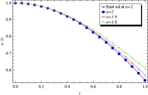
Table 1. Comparison between numerical results with exact solution at different α, N = 9.

t	Exact solution	Present method	Present method	Present method
	α = 2	α = 2	$\alpha =1.9$	$\alpha =1.8$
0.0	1.00000	1.00000	1.00000	1.00000
0.2	0.980067	0.980067	0.980067	0.980425
0.4	0.921061	0.921061	0.922065	0.924737
0.6	0.825336	0.825336	0.830344	0.839068
0.8	0.696707	0.696709	0.710747	0.731296
1.0	0.540302	0.540311	0.570531	0.610956

Example 3.

Consider the following linear FDIDE: (48) $$D^{\frac{7}{10}}u(t)+D^{\frac{1}{2}}u(t-1)+u\prime (t-1)+u^{″\prime }(t)=g(t)+\frac{1}{18}{\int }_0^{1}u(s)ds+\frac{1}{35}{\int }_{-1}^0{s}^{2}u(s)ds,$$(48) with the subjected conditions $u(0)=0,u\prime (0)=0,u″(0)=2,\epsilon =1,$ so $t\in [0,1],$ with the exact solution is $y(t)=t^2-t^4,$ by using (3) and (29) with $Q_0(t)=1,P_0(t)=1,P_1^{*}(t)=1,Q_3^{*}(t)=1,g(t)=-0.133333+2(-1+t)-4{(-1+t)}^3-2.06332(-1.8459+t)(-1.12951+t)(-0.524589+t)t^{0.5}-24t+0.334273(5.12821t^{1.3}-8.10783t^{3.3}),$ at N = 8 the fundamental matrix equation of the problem is defined by (49) $$\begin{array}{c}[Q_0 X_{{\nu }_0}{B}_{{\nu }_0}{L}^T+P_0 X_{{\alpha }_0}{B}_{{\alpha }_0}{B}_{-1}{L}^T+P_0^{*} XB B_{-1}{L}^T+Q_3^{*} X B^3{L}^T-{\beta }_0 H_0 L Z_0 L^T-{\beta }_1 H_1 L Z_1 L^T]A=G.\hfill \end{array}$$(49)

After we make all calculations for our problem, we can get the solution as: (50) $$A=\left[\begin{array}{ccccccccc}\frac{1}{8}& 0& \frac{1}{16}& 0& \frac{-1}{16}& 0& 0& 0& 0\end{array}\right].$$(50)

Therefor, the solution is of the problem (48)(48) $$D^{\frac{7}{10}}u(t)+D^{\frac{1}{2}}u(t-1)+u\prime (t-1)+u^{″\prime }(t)=g(t)+\frac{1}{18}{\int }_0^{1}u(s)ds+\frac{1}{35}{\int }_{-1}^0{s}^{2}u(s)ds,$$(48) (51) $$u_8(t)=\frac{1}{8}{U}_0(t)+\frac{1}{16}{U}_2(t)+\frac{-1}{16}{U}_4(t)=t^2-t^4.$$(51) which is the exact solution of the problem (48)(48) $$D^{\frac{7}{10}}u(t)+D^{\frac{1}{2}}u(t-1)+u\prime (t-1)+u^{″\prime }(t)=g(t)+\frac{1}{18}{\int }_0^{1}u(s)ds+\frac{1}{35}{\int }_{-1}^0{s}^{2}u(s)ds,$$(48) .

Example 4.

Consider the following linear FDIDE (Mohammed, 2014): (52) $$D^{1/2}u(t-\epsilon )=\frac{(8/3)t^{3/2}-2t^{1/2}}{\sqrt{\pi }}+\frac{t}{12}+{\int }_0^{1}s u(s)ds,\hspace{1em}-1+\epsilon \le t\le 1,$$(52) subject to $u(0)=0$ with the exact solution $u(t)=t^2-t$ at $\epsilon =0.$ By using (3)(3) $$u(t)\cong u_N(t)=\sum _{r=0}^N{A}_r{U}_r(t),$$(3) and (29)(29) $$t_j=\frac{-\epsilon }{2}\left(1+\hspace{0.17em}\text{cos}\hspace{0.17em}\left(\frac{\pi j}{N}\right)\right),j=0,1,2,\dots ,N.$$(29) with $Q_0(t)=1,$ at N = 8 the fundamental matrix equation of (52)(52) $$D^{1/2}u(t-\epsilon )=\frac{(8/3)t^{3/2}-2t^{1/2}}{\sqrt{\pi }}+\frac{t}{12}+{\int }_0^{1}s u(s)ds,\hspace{1em}-1+\epsilon \le t\le 1,$$(52) is: (53) $$\begin{array}{cc}\hfill & \left[Q_0 X_{{\nu }_0}{B}_{{\nu }_0}{L}^T-{\beta }_0 H_0 L Z_0 L^T\right]A=G.\hfill \end{array}$$(53)

After we make all calculations for our problem (when $\epsilon =0$), we can get the solution as: (54) $$A=\left[\begin{array}{ccccccccc}\frac{1}{4}& \frac{-1}{2}& \frac{1}{4}& 0& 0& 0& 0& 0& 0\end{array}\right].$$(54)

Then the solution is of Eq. (52)(52) $$D^{1/2}u(t-\epsilon )=\frac{(8/3)t^{3/2}-2t^{1/2}}{\sqrt{\pi }}+\frac{t}{12}+{\int }_0^{1}s u(s)ds,\hspace{1em}-1+\epsilon \le t\le 1,$$(52) (55) $$u_8(t)=\frac{1}{4}{U}_0(t)+\frac{-1}{2}{U}_1(t)+\frac{1}{4}{U}_2(t)=t^2-t.$$(55) which is the exact solution of the problem (52)(52) $$D^{1/2}u(t-\epsilon )=\frac{(8/3)t^{3/2}-2t^{1/2}}{\sqrt{\pi }}+\frac{t}{12}+{\int }_0^{1}s u(s)ds,\hspace{1em}-1+\epsilon \le t\le 1,$$(52) . A comparison between numerical results at different ε with the exact solution ($\epsilon =0$), N = 8 is listed in Table 2. Figure 2 shows the behavior of the numerical results with exact solution ($\epsilon =0$) at N = 8.

Figure 2. Comparison of the numerical results with exact solution at N = 8 for example 4.

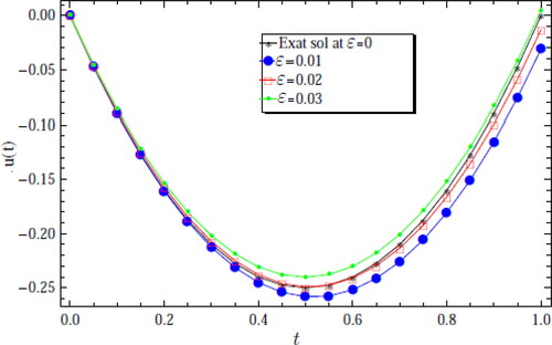
Table 2. Comparison between numerical results with the exact solution at different values of ε, N = 8 for example 4.

t	Exact solution	Present method	Present method	Present method
	$\epsilon =0$	$\epsilon =0.01$	$\epsilon =0.02$	$\epsilon =0.03$
0.0	0.00000	0.00000	0.00000	0.00000
0.2	−0.16000	−0.160769	−0.157172	−0.153576
0.4	−0.24000	−0.245119	−0.237903	−0.230698
0.6	−0.24000	−0.251869	−0.241074	−0.230300
0.8	−0.16000	−0.180557	−0.1662231	−0.151918
1.0	0.00000	−0.030929	−0.013094	0.0044010

Example 5.

Consider the following linear FIDE with delayed argument (Gülsu et al., 2010; Gürbüz, Sezer, & Güler, 2014): (56) $$\begin{array}{cc}\hfill & t D^{{\nu }_2}u(t)+t u^{\prime }(t)+u^{}(t-1)=f(t)+{\int }_0^1(\frac{12s^2}{7}-2) u(s) ds, t\in [0,1].\hfill \end{array}$$(56)

The initial conditions are $u(1)=1,u^{\prime }(1)=-2,$ and the exact solution is $u(t)=t^2-4t+4$ at ${\nu }_2=2,$ where $f(t)=\frac{14}{14}+{(-3+t)}^2+{(-2+t)}^2+2(-2+t)t-2t^2.$ We apply the suggested method with N = 4, then the fundamental matrix equation of the problem becomes as follows: (57) $$\begin{array}{cc}\hfill & \left[Q_2^{*}\hspace{0.17em}{X}_{}\hspace{0.17em}{B}^2\hspace{0.17em}{L}^T+Q_1^{*}\hspace{0.17em}{X}_1\hspace{0.17em}{B}^{}\hspace{0.17em}{L}^T+P_0^{*}\hspace{0.17em}{X}_{}\hspace{0.17em}{B}_{-1}\hspace{0.17em}\hspace{0.17em}{L}^T\hspace{0.17em}-{\beta }_0\hspace{0.17em}{H}_0\hspace{0.17em}L\hspace{0.17em}{Z}_0\hspace{0.17em}{L}^T\right]A=G,\hfill \end{array}$$(57)

Equation (57)(57) $$\begin{array}{cc}\hfill & \left[Q_2^{*}\hspace{0.17em}{X}_{}\hspace{0.17em}{B}^2\hspace{0.17em}{L}^T+Q_1^{*}\hspace{0.17em}{X}_1\hspace{0.17em}{B}^{}\hspace{0.17em}{L}^T+P_0^{*}\hspace{0.17em}{X}_{}\hspace{0.17em}{B}_{-1}\hspace{0.17em}\hspace{0.17em}{L}^T\hspace{0.17em}-{\beta }_0\hspace{0.17em}{H}_0\hspace{0.17em}L\hspace{0.17em}{Z}_0\hspace{0.17em}{L}^T\right]A=G,\hfill \end{array}$$(57) and condition are presents linear system of $(N+1)$ algebraic equations in the coeffcients c_i. The solution of this system gives the Chebyshev coefficients: $$A_0=\frac{9}{2}, A_1=-4, A_2=\frac{1}{2}, A_3=1.73868\times {10}^{-16}, A_4=-6.61509\times {10}^{-18}.$$

Thus, the approximate solution of this problem becomes. (58) $$u_4(t)=\frac{9}{4}{U}_0(t)-4U_1(t)+\frac{1}{2}{U}_2(t)+1.73868\times {10}^{-16}{U}_3(t)-6.61509\times {10}^{-18}{U}_4(t).$$(58)

A comparison between the absolute errors for the present method at N = 4 with results in Gürbüz et al. (2014) at N = 8 and N = 10 is listed in Table 3. Table 4 shows the comparison of the numerical solution of the present method at N = 4 and results in Gürbüz et al. (2014) with the exact solution. Figure 3 shows the comparison of the present method numerical results of u(t) at different values of ν for N = 4 with exact solution (v = 2).

Figure 3. Comparison of u(t) for N = 4 with ν = 2, 1.8,1.7, 1.6 for example 5.

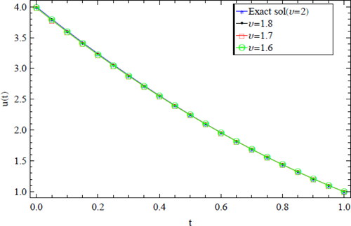
Table 3. Comparison of the absolute errors for example 5 for different N values at ν = 2.

t	Present method N = 4	Ref Gürbüz et al. (2014) at N = 8	Ref Gürbüz et al. (2014) at N = 10
0	9.4896$\times {10}^{-17}$	0.67000$\times {10}^{-15}$	0.12300$\times {10}^{-12}$
0.1	1.5421$\times {10}^{-16}$	0.22193$\times {10}^{-2}$	0.39880$\times {10}^{-4}$
0.2	8.88178$\times {10}^{-17}$	0.95897$\times {10}^{-2}$	0.22276$\times {10}^{-3}$
0.3	2.2321$\times {10}^{-14}$	0.22995$\times {10}^{-1}$	0.87128$\times {10}^{-3}$
0.4	7.2417$\times {10}^{-15}$	0.70446$\times {10}^{-1}$	0.20625$\times {10}^{-2}$

Table 4. Numerical solution of example 5 for different N values.

t	Exact solution	Present method N = 4	Ref Gürbüz et al. (2014) at N = 8
0	4.000000	4.000000	4.000000
0.1	3.610000	3.610000	3.607781
0.2	3.240000	3.240000	3.230410
0.3	2.890000	2.890000	2.867005
0.4	2.560000	2.560000	2.779554

7. Conclusion

In this paper, a numerical solution of general form of linear fractional delay integro-differential equation (GFDIDE) is presented using spectral collocation method. The proposed equation represents a general form of intgro-differential equations with delayed argument, which has multi-terms of delayed or non-delayed terms with integer and fractional order derivatives for these terms. The Chebyshev polynomials of the second kind are used as a basis function with the collocation method for GFDIDEs. The collocation scheme reduces the proposed equation to system of algebraic equation. The operational matrices for all terms of GFDIDE according to the fractional calculus are introduced. The accuracy and competence of the suggested scheme have been explained by some numerical examples.

Authors’ contributions

E. M. H. Mohamed suggested the point for this paper and modified the manuscript and arranged it in its final form. K. R. Raslan performed the examples on the computer packge. K. K. Ali and M. A. Abd El Salam revised the mathematical research point and helped in coding using Mathematica program. All authors contributed to the manuscript writing, read and approved the final manuscript.

Disclosure statement

No potential conflict of interest was reported by the authors.

References

- Ahmad, H., & Khan, T. A. (2020). Variational iteration algorithm I with an auxiliary parameter for the solution of differential equations of motion for simple and damped mass–spring systems. Noise & Vibration Worldwide, 51(1–2), 12–20. doi:10.1177/0957456519889958
- Ahmad, H., Khan, T. A., & Cesarano, C. (2019). Numerical solutions of coupled Burgers’ equations. Axioms, 8(4), 119. doi:10.3390/axioms8040119
- Ahmad, H., Seadawy, A. R., & Khan, T. A. (2020). Numerical solution of Korteweg–de Vries-Burgers equation by the modified variational iteration algorithm-II arising in shallow water waves. Physica Scripta, 95(4), 045210. doi:10.1088/1402-4896/ab6070
- Ahmad, H., Seadawy, A. R., Khan, T. A., & Thounthong, P. (2020). Analytic approximate solutions for some nonlinear Parabolic dynamical wave equations. Journal of Taibah University for Science, 14(1), 346–358. doi:10.1080/16583655.2020.1741943
- Akyuz, A., & Sezer, M. (2003). Chebyshev polynomial solutions of systems of high-order linear differential equations with variable coefficients. Applied Mathematics and Computation, 144(2–3), 237–247. doi:10.1016/S0096-3003(02)00403-4
- Ali, K. K., El Salam, M. A. A., & Mohamed, E. M. (2019). Chebyshev operational matrix for solving fractional order delay-differential equations using spectral collocation method. Arab Journal of Basic and Applied Sciences, 26(1), 342–353. doi:10.1080/25765299.2019.1629543
- Bhrawy, A. H., Alofi, A. S., & Ezz-Eldien, S. S. (2011). A quadrature tau method for fractional differential equations with variable coefficients. Applied Mathematics Letters, 24(12), 2146–2152. doi:10.1016/j.aml.2011.06.016
- Doha, E. H., Bhrawy, A. H., & Ezz-Eldien, S. S. (2011). A Chebyshev spectral method based on operational matrix for initial and boundary value problems of fractional order. Computers & Mathematics with Applications, 62(5), 2364–2373. doi:10.1016/j.camwa.2011.07.024
- Doha, E. H., Bhrawy, A. H., & Saker, M. A. (2011). Integrals of Bernstein polynomials: An application for the solution of high even-order differential equations. Applied Mathematics Letters, 24(4), 559–565. doi:10.1016/j.aml.2010.11.013
- Fang, J. J., & Dai, C. Q. (2020). Optical solitons of a time-fractional higher-order nonlinear Schrödinger equation. Optik, 209, 164574. doi:10.1016/j.ijleo.2020.164574
- Gökdoğan, A., Merdan, M., & Ertürk, V. S. (2013). A multistage variational iteration method for solution of delay differential equations. International Journal of Nonlinear Sciences and Numerical Simulation, 14(3–4), 159–166. doi:10.1515/ijnsns-2011-0180
- Gokdogan, A., Merdan, M., & Yildirim, A. (2012). Differential transformation method for solving a neutral functional-differential equation with proportional delays. Caspian Journal of Mathematical Sciences (CJMS), 1, 1.
- Gülsu, M., Öztürk, Y., & Sezer, M. (2010). A new collocation method for solution of mixed linear integro-differential-difference equations. Applied Mathematics and Computation, 216(7), 2183–2198. doi:10.1016/j.amc.2010.03.054
- Gürbüz, B., Sezer, M., & Güler, C. (2014). Laguerre collocation method for solving Fredholm integro-differential equations with functional arguments. Journal of Applied Mathematics, 2014, 1–12. doi:10.1155/2014/682398
- He, J. H. (2000). review on some new recently developed nonlinear analytical techniques. International Journal of Nonlinear Sciences and Numerical Simulation, 1(1), 51–70. doi:10.1515/IJNSNS.2000.1.1.51
- He, J. H. (2019). The simpler, the better: Analytical methods for nonlinear oscillators and fractional oscillators. Journal of Low Frequency Noise, Vibration and Active Control, 38(3–4), 1252–1260. doi:10.1177/1461348419844145
- He, J. H. (2020). Taylor series solution for a third order boundary value problem arising in Architectural Engineering. Ain Shams Engineering Journal. In Press. doi:10.1016/j.asej.2020.01.016
- He, J. H., & Latifizadeh, H. (2020). A general numerical algorithm for nonlinear differential equations by the variational iteration method. International Journal of Numerical Methods for Heat & Fluid Flow. In Press. doi:10.1108/HFF-01-2020-0029
- Khader, M. M., & Hendy, A. S. (2012). The approximate and exact solution of the fractional order delay differential equations using Legendre pseudo spectral method. International Journal of Pure and Applied Mathematics, 74(3), 287–297.
- Khader, M. M., & Saad, K. M. (2018). A numerical approach for solving the fractional Fisher equation using Chebyshev spectral collocation method. Chaos, Solitons & Fractals: X, 110, 169–177. doi:10.1016/j.chaos.2018.03.018
- Mohammed, D. S. (2014). Numerical solution of fractional integro-differential equations by least squares method and shifted Chebyshev polynomial. Mathematical Problems in Engineering, 2014, 1–5. Article ID 431965. doi:10.1155/2014/431965
- Morgado, M. L., Ford, N. J., & Lima, P. M. (2013). Analysis and numerical methods for fractional differential equations with delay. Journal of Computational and Applied Mathematics, 252, 159–168. doi:10.1016/j.cam.2012.06.034
- Muthukumar, P., & Ganesh Priya, B. (2017). Numerical solution of fractional delay differential equation by shifted Jacobi polynomials. International Journal of Computer Mathematics, 94(3), 471–492. doi:10.1080/00207160.2015.1114610
- Rahimkhani, P., Ordokhani, Y., & Babolian, E. (2017). A new operational matrix based on Bernoulli wavelets for solving fractional delay differential equations. Numerical Algorithms, 74(1), 223–245. doi:10.1007/s11075-016-0146-3
- Ramadan, M. A., & Abd El Salam, M. A. (2016). Solving systems of ordinary differential equations in unbounded domains by exponential Chebyshev collocation method. Journal of Abstract and Computational Mathematics, 1, 33–46.
- Ramadan, M. A., Raslan, K. R., El Danaf, T. S., & Abd El Salam, M. A. (2017). An exponential Chebyshev second kind approximation for solving high-order ordinary differential equations in unbounded domains, with application to Dawson’s integral. Journal of the Egyptian Mathematical Society, 25(2), 197–205. doi:10.1016/j.joems.2016.07.001
- Raslan, K. R., Abd El Salam, M. A., Ali, K. K., & Mohamed, E. M. (2019). Spectral Tau method for solving general fractional order differential equations with linear functional argument. Journal of the Egyptian Mathematical Society, 27(1), 33. doi:10.1186/s42787-019-0039-4
- Saeed, U., & Ur Rehman, M. (2014). Hermite Wavelet method for fractional delay differential equations. Journal of Difference Equations, 2014, 1–8. Article ID 359093. doi:10.1155/2014/359093
- Siyyam, I. H. (2011). Laguerre tau methods for solving higher-order ordinary differential equations. Journal of Computational Analysis and Applications, 3(2), 173–182.
- Ur Rehman, M., & Ali Khan, R. (2011). The Legendre wavelet method for solving fractional differential equations. Communications in Nonlinear Science and Numerical Simulation, 16(11), 4163–4173. doi:10.1016/j.cnsns.2011.01.014
- Wang, B. H., Lu, P. H., Dai, C. Q., & Chen, Y. X. (2020). Vector optical soliton and periodic solutions of a coupled fractional nonlinear Schrödinger equation. Results in Physics, 17, 103036. doi:10.1016/j.rinp.2020.103036
- Wang, Z., & Guo, B. (2012). Legendre-Gauss-Radau collocation method for solving initial value problems of first order ordinary differential equations. Journal of Scientific Computing, 52(1), 226–255. doi:10.1007/s10915-011-9538-7
- Wu, G. Z., & Dai, C. Q. (2020). Nonautonomous soliton solutions of variable-coefficient fractional nonlinear Schrödinger equation. Applied Mathematics Letters, 106, 106365. doi:10.1016/j.aml.2020.106365
- Wu, G. Z., Yu, L. J., & Wang, Y. Y. (2020). Fractional optical solitons of the space-time fractional nonlinear Schrödinger equation. Optik, 207, 164405. doi:10.1016/j.ijleo.2020.164405
- Xu, M.-Q., & Lin, Y.-Z. (2016). Ying-Zhen Lin Simplified reproducing kernel method for fractional differential equations with delay. Applied Mathematics Letters, 52, 156–161. doi:10.1016/j.aml.2015.09.004
- Yang, C. (2012). Chebyshev polynomial solution of nonlinear integral equations. Journal of the Franklin Institute, 349(3), 947–956. doi:10.1016/j.jfranklin.2011.10.023
- Yu, D. N., He, J. H., & García, A. G. (2019). Homotopy perturbation method with an auxiliary parameter for nonlinear oscillators. Journal of Low Frequency Noise, Vibration and Active Control, 38(3–4), 1540–1554. doi:10.1177/1461348418811028