Existence theory and numerical simulation of ebola model corresponding to nonlocal fractional order derivative

Abstract

In this article, the qualitative theory and approximate solutions for fractional order Ebola model via Atangana-Baleanu-Caputo (ABC) fractional operators are developed. Using various tools of analysis, the conditions for the existence and stability of the proposed model are established. With the help of Laplace Adomain Decomposition method, we obtain the approximate solutions for the said model. In the last part, using Matlab, we plotted various graphs to discuss the underlying model for different fractional order values of γ.

Keywords:

• Approximate solutions
• fixed point theory
• fractional derivatives
• Laplace-Adomian decomposition method
• mathematical modelling
• Ulams type stabilities

AMS SUBJECT CLASSIFICATION:

• 26A33
• 34A08
• 93A30

1. Introduction

Modern experimental evidences confirm that natural dynamics follow fractional calculus, which is a fastest growing area of research having applications in diverse and widespread fields of engineering and science such as electromagnetic, viscoelasticity, signal and image processing, quantum mechanics, control theory, non-linear dynamics, biological population models, and optimization theory (Hilfer, 2000; Kilbas, Marichev, & Samko, 1993; Kilbas, Srivastava, & Trujillo, 2006; Miller & Ross, 1993; Podlubny, 1999; Rahimkhani, Ordokhani, & Babolian, 2017; Saeed & Rehman, 2014; Yang & Huang, 2013; Zhou, 2016). Dealing with the dynamical system, having memory effects, is one of the biggest challenges for researchers. Since the fractional calculus has direct link with the dynamical system with memory effect. Therefore, Fractional Differential Equations (FDEs), which is a novel technique, is developed to model phenomena related to the dynamics of the aforesaid fields of science (Ali, Samet, Shah, & Khan, 2017; Ali, Shah, & Khan, 2016; Caputo, 1967; Lakshmikantham, Leela, & Vasundhara, 2009). FDEs are global in nature and possess greater degree of freedom as compared to the conventional differential equations (DEs). Owing to this extraordinary property, numerous researchers have investigated various features of FDEs concerning the existence, stability analysis, and approximate solutions. The researchers utilized different techniques of fixed-point theory and numerical analysis so as to investigate the existence theory, stability analysis, and approximate solution of FDEs that refers to Agarwal, Belmekki, and Benchohra (2009), Akram and Tariq (2018), Cai and Wu (2009), Nanware and Dhaigude (2014) and Wu, Hei, and Chen (2013). It is note worthy that stability analysis and approximate solutions are the key factors of FDEs. In various real-world problems, either it is quite difficult or complicated and massive calculations are required to obtain the exact solution of FDEs. In like circumstances, stability analysis and approximate solutions play an inevitable role to tackle the complicated problems involving FDEs. Despite the fact that there are verities of stabilities such as Lyapunov Stability, Exponential Stability, Asymptotic Stability, Mittag-Leffler Stability (Lijun, Wang, & Wang, 2015; Stamova, 2015; Trigeassou, Maamri, Sabatier, & Oustaloup, 2011; Ullam, 1940), the most reliable one is Ullam-Hyers (UH) Stability, which is the consequent of the correspondence between Ullam (1940) and Hyers (1941). The UH stability was further modified and generalized by various other researchers (Rassias, 1978; Ulam, 1960).

Like classical derivatives of calculus, fractional calculus also involves various types of fractional derivatives such as Riemann-Liouville (RL), Caputo (C), Hamdard (H), Caputo Febrizo (CF), Atangana-Baleanu (AB) and Atangana-Baleanu-Caputo (ABC). The derivatives in sense of Riemann-Liouville and Caputo are broadly used and well explored by several researchers (Benchohra, Hamani, & Ntouyas, 2009; Khan & Shah, 2015; Shah & Khan, 2015). Since the classical fractional derivatives involving a singular kernel, could not determine the nonlocal dynamics. Therefore, the notion of non-singular derivatives has been introduced. In 2016, Caputo and Fabrizo contributed non-singular derivative involving exponential function. In subsequent years, the concerned derivative were generalized by Atangana-Baleanu-Caputo, which is known as ABC derivative. The operator is recently construed non-local, without singular kernel and reliable differential operator, which are applied in modelling of various real-world phenomena (Atangana & Baleanu, 2016). The complex situations, due to singular kernel, have been replaced by exponential and power decay law, for detail see (Algahtani, 2016; Djida, Atangana, & Area, 2017). The problems under ABC derivative have been studied for iterative solutions mostly by using some integral transform, but very rarely investigated from qualitative and numerical aspects.

Laplace Transform is an integral transform, which is used in various biological and engineering problems. More precisely, it is an influential tool to solve a verity of FDEs with initial conditions. Additionally, it is used for the interpretation of time invariant systems such as harmonic oscillation, electric circuit, mechanical systems and optical devices. In addition, it is used to change the problem from time domain to frequency domain. Using Laplace Transform, a differential equation is converted to an algebraic equation, which can be solved through algebraic techniques. Moreover, the Laplace Transform is invertible. The Inverse Laplace Transform takes a function of complex variable and yield a function of real variables. A verity of numerical computational techniques such as Homotopy Perturbation Method (HPM) (Kumar, Singh, & Kumar, 2015), Variation Iteration Method (VIM) (Yang, Xiao, & Su, 2010), Generalized Differential Method (GDM) (Odibat & Momani, 2008), Homotopy Variation Iteration Method (HVIM) (Deghan, Yousefi, & Lotfi, 2011), New Homotopy Analysis Transform Method (NHATM) (Maitama & Zhao, 2020) and Adomain Decomposition Method (ADM) are being used. One of the most accurate and efficient approximate technique for the solution of FDEs is Laplace Transform, which is coupled with ADM and is recognized as Laplace Adomian Decomposition Method (LADM). The said technique is a powerful tool to obtain numerical solutions of wide range of initial and boundary value problems of FDEs. It provides the solutions of an infinite series in which each term can be determined easily.

In real world situation, either to study the biological behaviours of diseases accurately or to precisely tackle an engineering problem, a powerful mathematical tool, which produces more reliable results, is known as mathematical modelling. In this regard, various mathematical modelling tools have been used to study the transmission and developed a better plane for the prevention of mankind from these deadly infectious diseases, see (Beauchemin & Handel, 2011; Edelstein-Keshet, 2005; Zhou et al., 2020). It has been observed that proper understanding and implementation for the control strategies against the transmission of spreading diseases in the community is unbreakable challenge for mankind. To some extent, the aforementioned techniques play a key role to plane, prevent and eliminate the deadly diseases from the community. The readers further refer to (Brauer, Driessche, & Wu, 2008; Murray, 2007; Rvachev, Ira, & Longini, 1985).

In the year 1976, an outbreak took place in African country of the Democratic Republic of Congo (DRC), which was named as Ebola outbreak where a deadly virus spread dramatically. The virus was named after the river Ebola flow near the DRC. The virus has five types out of which four cause diseases in humans. The virus used to attack on the immune system and resultantly inner bleeding took place that damaged every organ of the body. This scary virus spread through direct contact with infected person either through body fluids or skin interaction. The virus could also be transmitted through interaction with the infected animals like monkey, chimp or fruit bat. The people who were taking care or buried the infected person were the easy targets of the virus. However, the virus cannot be spread through air, water and food. Interestingly, the infected person with no symptoms could not transmit the virus to others. Later on, in 2013, the virus emerged in Guckduo and Guinea (Lamb, 2013), where 28,616 cases were reported out of which 11,310 reported as dead. To study the dynamics of the virus, several mathematicians have tried their best to discuss the transmission and biological behaviour of the virus for details refer to (Bowen et al., 1977; Kuhn et al., 2010; Pattyn et al., 1977; Tahir, Shah, Zaman, & Khan, 2019).

Today, where the modern world is facing another pandemic outbreak in the form of corona virus, the study of such infectious diseases is still a central focus for the researchers. In this regard, we predicted and investigated the dynamics of fractional order Ebola model (1) via ABC fractional operator. We developed a precise mechanism how to prevent the transmission of infectious disease in the community. The capture fractional order Ebola under Atangaba-Baleau-Caputo derivative is given as: (1) $$\begin{array}{c}{}^{\mathit{ABC}}{D}^{\gamma }S(t)=\frac{\alpha }{2}-\lambda S(t)-\frac{\tau }{\alpha }S(t)E(t)-({\theta }_1+{\theta }_2)S(t)I(t),\hfill \\ {}^{\mathit{ABC}}{D}^{\gamma }E(t)=\tau S(t)E(t)-mE(t)I(T)-(n_1+n_2)E(t),\hfill \\ {}^{\mathit{ABC}}{D}^{\gamma }I(t)=mE(t)I(t)+({\theta }_1+{\theta }_2)S(t)I(t)\hfill \\ -\frac{\eta }{\lambda }I(t)R(t)-({\beta }_1+{\beta }_2)I(t),\hfill \\ {}^{\mathit{ABC}}{D}^{\gamma }V(t)=({\beta }_1+{\beta }_2)I(t)-\kappa V(t),\hfill \\ {}^{\mathit{ABC}}{D}^{\gamma }R(t)=\frac{\eta }{\lambda }I(t)-\rho R(t).\hfill \end{array}$$(1)

With initial conditions $S(0)=S_0, E(0)=E_0, I(0)=I_0, V(0)=V_0$ and $R(0)=R_0,$ where $0<\gamma \le 1.$

The parameters involved in (1) and their physical interpretation is expressed in Table 1. Here we also assume that all the parameters are non-negative.

Table 1. Description of the parameters used in model (1).

Parameters	The physical interpretation
S(t)	Susceptible people
E(t)	Exposed people
I(t)	Infected people
V(t)	Vaccinated people
R(t)	Recovered people
$\alpha , \lambda$	Symbolize new birth and death rate in susceptible people
θ1	Symbolize Infection transmission rate from susceptible people to infected people through
	via animals infections
θ2	Symbolize Infection transmission rate from susceptible people to infected people via
	domestic animals
τ	Symbolize infection transmission rate from susceptible people to exposed people
m	Symbolize infection transmission rate from exposed people to infected people
η	Symbolize recovery rate in recovered people
$n_1, n_2$	Symbolize natural and infectious death rate in exposed people
${\beta }_1, {\beta }_2$	Symbolize natural and infectious death rate in infected people
ρ	Symbolize natural death rate of recovered people

Corresponding to model (1), we use fixed point approach to investigate some results that ensure the existence of such model and its solution. We use Banach and Schauder’s theorems from fixed point theory. We obtain the estimated solution of concerned model of non-integer order via Laplace transform combined with Adomian decomposition method. To justified the results obtained by aforementioned procedure, we use Mapple-13 and assigned different values to the parameters and supplement conditions.

An efficient techniques by which we can find both explicit and analytic solutions for the system of differential equations, was initiated by Adomain is known as LADM, in 1980. The aforesaid techniques have an efficient techniques, which works outstandingly in both cases that is initial and boundary value problems. The consider method also works accurately in a system of stochastic differential equations. LADM does not needs liberalization or perturbation, like other existing computational and analytical schemes, that needs for exploring the dynamical behaviour of complex dynamical systems. The committed techniques provide extensive results for the solutions of Fractional Order Differential Equations (FODEs) and as well as for analytical solution for the verity problem of nonlinear equations. In this paper, we utilized techniques of Adomain polynomial to decomposed the non-linearity and Laplace to convert the deserts problem to the form algebraic equations, see Biazar (2006). Recently, the proposed techniques are used to deal with non-singular FODEs, to obtained very fruitful results (see Shah, Alqudah, Jarad, & Abdelijawad, 2020). Furthermore, we remark that the obtained results via the considered method is in a form of convergent series, that converges to the exact results uniformly. Thanks to the results of analysis (Abdilraze & Pelinosky, 2009; Naghipour & Manafian, 2015; Shah, Khalil, & Khan, 2018), one can easily prove the convergent of the proposed method.

2. Preliminaries

Definition 2.1.

If $\Psi (t)\in {\mathbb{H}}^1(0,\mathcal{T})$ and $\gamma \in (0,1],$ then the $\mathcal{A}\mathcal{B}\mathcal{C}$ derivative is defined as (2) $${}^{\mathit{ABC}}{D}_{+0}^{\gamma }\Psi (t)=\frac{M(\gamma )}{1-\gamma }{\int }_0^t\frac{d}{dx}\Psi (y)M_{\gamma }[\frac{-\gamma }{1-\gamma }(t-y)]dy,$$(2) if we replace $M_{\gamma }[\frac{-\gamma }{1-\gamma }(t-y)]dy$ by $M_1=\hspace{0.17em}\text{exp}[\frac{-\gamma }{1-\gamma }(t-y)],$ then we get the Caputo-Fabrizo differential operator. It is to be noted that $${}^{\mathit{ABC}}{D}_{+0}^{\gamma }\left[\mathit{Constant}\right]=0,$$ where $M(\gamma )$ is known as normalization function which is defined as $\mathit{ABC}(0)=\mathit{ABC}(1)=1.$ $M_{\gamma }$ stands for famous function known as Mittag-Leffler, the generalization of exponential function (Rafei, Ganji, & Daniali, 2007).

Definition 2.2.

Let $z\in L[0,T],$ Then the integral in sense of ABC is defined as (3) $${}^{\mathit{ABC}}{D}_{+0}^{\gamma }z(t)=\frac{1-\gamma }{M(\gamma )}z(t)+\frac{\gamma }{M(\gamma )\Gamma (\gamma )}{\int }_0^t{(t-y)}^{\gamma -1}z(y)dy.$$(3)

Lemma 2.1.

Ali, Zada, and Shah (2018) solution of the problem for $1>\gamma >0$ $$\begin{array}{cc}\hfill & {}^{\mathit{ABC}}{D}_{+0}^{\gamma }U(t)=x(t), t\in [0,T],\hfill \\ \hfill & U(0)=U_0\hfill \end{array}$$ is given by $$U(t)=U_0+\frac{(1-\gamma )}{M(\gamma )}x(t)+\frac{\gamma }{\Gamma (\gamma )M(\gamma )}{\int }_0^t{(t-y)}^{\gamma -1}x(y)dy.$$

Definition 2.3.

Laplace transform for ABC derivative of function $\varphi (t)$ is given by $$ℒ{[}^{\mathit{ABC}}{D}_0^{\gamma }\varphi (t)]=\frac{M(\gamma )}{s^{\gamma }(1-\gamma )+\gamma }[s^{\gamma }ℒ[\varphi (t)]-s^{\gamma -1}\varphi (0)].$$

Key point: For qualitative analysis, we define Banach space $\mathbb{Z}=\mathbb{X}\times \mathbb{X}\times \mathbb{X}\times \mathbb{X}\times \mathbb{X},$ with $\mathbb{X}=C[0,T]$ under the norm defined by $\left|\right|M\left|\right|=\left|\right|(S,E,I,V,R)\left|\right|=ma{x}_t\in [0,T]\left|\right|S(t)+E(t)+I(t)+V(t)+R(t)\left|\right|.$ For our main result, the following theorem will be used.

Theorem 2.4.

Let $\mathbb{B}$ be a convex subset of $\mathbb{Z}$, assuming that $\mathbb{F},\mathbb{G}$ are two operators with

(1). $\mathbb{F}u+\mathbb{G}u\in \mathbb{B}$ for every $u\in \mathbb{B}.$

(2). $\mathbb{F}$ is contraction.

(3). $\mathbb{G}$ is continuous and compact.

Then the operator equation $\mathbb{F}u+\mathbb{G}u=u$, has at least one solution.

3. Existence theory

The concerned section, is dedicated to the existence and uniqueness of the solution of considered model of FDEs. FDEs provide powerful tools, that describes different physical, biological and dynamical phenomenon in mathematical concepts. In last two decades, due to the versatile applications of FDEs, the researchers give more attention to the existence of solutions for FDEs. Another important aspects of FDEs, that it is widely used in the different fields of applied science and technology is devoted to the stability analysis. In this section we determined existence result for the proposed model (1), using fixed point theorem due to Banach type for the existence and uniqueness of solution. In this regard, we first define the following function (4) $$\{\begin{array}{c}{\psi }_1\left(t,S,E,I,V,R\right)=\frac{\alpha }{2}-\lambda S(t)-\frac{\tau }{\alpha }S(t)E(t)-({\theta }_1+{\theta }_2)S(t)I(t),\hfill \\ {\psi }_2\left(t,S,E,I,V,R\right)=\tau S(t)E(t)-mE(t)I(T)-(n_1+n_2)E(t),\hfill \\ {\psi }_3\left(t,S,E,I,V,R\right)=mE(t)I(t)+({\theta }_1+{\theta }_2)S(t)I(t)\hfill \\ -\frac{\eta }{\lambda }I(t)R(t)-({\beta }_1+{\beta }_2)I(t),\hfill \\ {\psi }_4\left(t,S,E,I,V,R\right)=({\beta }_1+{\beta }_2)I(t)-\kappa V(t),\hfill \\ {\psi }_5\left(t,S,E,I,V,R\right)=\frac{\eta }{\lambda }I(t)-\rho R(t).\hfill \end{array}$$(4)

With the help of (4)(4) $$\{\begin{array}{c}{\psi }_1\left(t,S,E,I,V,R\right)=\frac{\alpha }{2}-\lambda S(t)-\frac{\tau }{\alpha }S(t)E(t)-({\theta }_1+{\theta }_2)S(t)I(t),\hfill \\ {\psi }_2\left(t,S,E,I,V,R\right)=\tau S(t)E(t)-mE(t)I(T)-(n_1+n_2)E(t),\hfill \\ {\psi }_3\left(t,S,E,I,V,R\right)=mE(t)I(t)+({\theta }_1+{\theta }_2)S(t)I(t)\hfill \\ -\frac{\eta }{\lambda }I(t)R(t)-({\beta }_1+{\beta }_2)I(t),\hfill \\ {\psi }_4\left(t,S,E,I,V,R\right)=({\beta }_1+{\beta }_2)I(t)-\kappa V(t),\hfill \\ {\psi }_5\left(t,S,E,I,V,R\right)=\frac{\eta }{\lambda }I(t)-\rho R(t).\hfill \end{array}$$(4) , the constructed system is written in the following form (5) $$\begin{array}{cc}\hfill & {}^{\mathit{ABC}}{D}_{+0}^{\gamma }U(t)=\psi (t,U(t)), t\in [0,T], 0<\gamma \le 1,\hfill \\ \hfill & U(0)=U_0.\hfill \end{array}$$(5)

Using Lemma (2.1), Equation (5)(5) $$\begin{array}{cc}\hfill & {}^{\mathit{ABC}}{D}_{+0}^{\gamma }U(t)=\psi (t,U(t)), t\in [0,T], 0<\gamma \le 1,\hfill \\ \hfill & U(0)=U_0.\hfill \end{array}$$(5) becomes (6) $$U(t)=U_0(t)+[\psi ((t,U(t))-{\psi }_0(t)]\frac{1-\gamma }{M(\gamma )}+\frac{\gamma }{M(\gamma )\Gamma (\gamma )}{\int }_0^t{(t-y)}^{\gamma -1}\psi (y,U(y))dy, \mathit{for} 0\le y\le t\le 1,$$(6) where (7) $$U(t)=\{\begin{array}{c}S(t)\hfill \\ E(t)\hfill \\ I(t)\hfill \\ V(t)\hfill \\ R(t)\hfill \end{array},U_0(t)=\{\begin{array}{c}{S}_0\hfill \\ E_0\hfill \\ I_0\hfill \\ V_0\hfill \\ R_0\hfill \end{array},\psi (t,U(t))=\{\begin{array}{c}{\psi }_1(t,S,E,I,V,R)\hfill \\ {\psi }_2(t,S,E,I,V,R)\hfill \\ {\psi }_3(t,S,E,I,V,R)\hfill \\ {\psi }_4(t,S,E,I,V,R)\hfill \\ {\psi }_5(t,S,E,I,V,R)\hfill \end{array},{\psi }_0(t)\{\begin{array}{c}{\psi }_1(0,S_0,E_0,I_0,V_0,R_0)\hfill \\ {\psi }_2(0,S_0,E_0,I_0,V_0,R_0)\hfill \\ {\psi }_3(0,S_0,E_0,I_0,V_0,R_0)\hfill \\ {\psi }_4(0,S_0,E_0,I_0,V_0,R_0)\hfill \\ {\psi }_5(0,S_0,E_0,I_0,V_0,R_0)\hfill \end{array}.$$(7)

Using (6)(6) $$U(t)=U_0(t)+[\psi ((t,U(t))-{\psi }_0(t)]\frac{1-\gamma }{M(\gamma )}+\frac{\gamma }{M(\gamma )\Gamma (\gamma )}{\int }_0^t{(t-y)}^{\gamma -1}\psi (y,U(y))dy, \mathit{for} 0\le y\le t\le 1,$$(6) and (7)(7) $$U(t)=\{\begin{array}{c}S(t)\hfill \\ E(t)\hfill \\ I(t)\hfill \\ V(t)\hfill \\ R(t)\hfill \end{array},U_0(t)=\{\begin{array}{c}{S}_0\hfill \\ E_0\hfill \\ I_0\hfill \\ V_0\hfill \\ R_0\hfill \end{array},\psi (t,U(t))=\{\begin{array}{c}{\psi }_1(t,S,E,I,V,R)\hfill \\ {\psi }_2(t,S,E,I,V,R)\hfill \\ {\psi }_3(t,S,E,I,V,R)\hfill \\ {\psi }_4(t,S,E,I,V,R)\hfill \\ {\psi }_5(t,S,E,I,V,R)\hfill \end{array},{\psi }_0(t)\{\begin{array}{c}{\psi }_1(0,S_0,E_0,I_0,V_0,R_0)\hfill \\ {\psi }_2(0,S_0,E_0,I_0,V_0,R_0)\hfill \\ {\psi }_3(0,S_0,E_0,I_0,V_0,R_0)\hfill \\ {\psi }_4(0,S_0,E_0,I_0,V_0,R_0)\hfill \\ {\psi }_5(0,S_0,E_0,I_0,V_0,R_0)\hfill \end{array}.$$(7) , define two operators $\mathbb{F}$ and $\mathbb{G},$ using (6)(6) $$U(t)=U_0(t)+[\psi ((t,U(t))-{\psi }_0(t)]\frac{1-\gamma }{M(\gamma )}+\frac{\gamma }{M(\gamma )\Gamma (\gamma )}{\int }_0^t{(t-y)}^{\gamma -1}\psi (y,U(y))dy, \mathit{for} 0\le y\le t\le 1,$$(6) (8) $$\begin{array}{cc}\hfill & \mathbb{F}u=U_0(t)+[\psi (t,U(t))-{\psi }_0(t)]\frac{1-\gamma }{M(\gamma )},\hfill \\ \hfill & \mathbb{G}u=\frac{\gamma }{M(\gamma )\Gamma (\gamma )}{\int }_0^t{(t-y)}^{\gamma -1}\psi (y,U(y))dy.\hfill \end{array}$$(8)

For growth condition, Lipschitizian assumptions, existence and uniqueness, the following holds

$(L_1)$ There exists constants $b^{*}$ and $c^{*},$ such that $$|\psi (t,U(t))|\le b^{*}|U(t)|+c^{*}.$$ $(L_2)$ There exists constant K_p > 0, for every $u,u_1\in \mathbb{X},$ such that $$|\psi (t,U(t))-\psi (t,U_1(t))|\le K_p\left|\right|u-u_1\left|\right|.$$

Theorem 3.1.

If $(L_1)$ and $(L_2)$ holds, then Equation (6) has at least one solution which means that the consider system (1) has one solution if $$\frac{(1-\gamma )K_p}{M(\gamma )}<1.$$

Proof.

To show that $\mathbb{F}$ is contraction, let $u_1\in \mathbb{B},$ where $\mathbb{B}=\{u\in \mathbb{Z}:|\left|u\right||\le r,r>0\}$ is closed convex set. Using the definition of $\mathbb{F}$ from (8), we get (9) $$\begin{array}{cc}\hfill & \left|\right|\mathbb{F}u-\mathbb{F}{u}_1\left|\right|=\frac{(1-\gamma )}{M(\gamma )}\underset{t\in [0,T]}{\max }|\psi (t,U(t))-\psi (t,U_1(t))|,\hfill \\ \hfill & \le \frac{{(1-\gamma )}_p}{M(\gamma )}\left|\right|u-u_1\left|\right|.\hfill \end{array}$$(9)

Hence $\mathbb{F}$ is contraction.

To show that $\mathbb{G}$ is relatively compact, we have to show that $\mathbb{G}$ is bounded, and continuous. For this, we proceeds as follow:

It is obvious that $\mathbb{G}$ is continuous as ψ is continuous, also for $u\in \mathbb{B},$ we have (10) $$\begin{array}{cc}\hfill & |\mathbb{G}(u)|=\underset{t\in [0,T]}{\max }\frac{\gamma }{M(\gamma )\Gamma (\gamma )}\left|\right|{\int }_0^t{(t-y)}^{\gamma -1}\psi (y,U(y))dy\left|\right|,\hfill \\ \hfill & \le \frac{\gamma }{M(\gamma )\Gamma (\gamma )}{\int }_0^T{(T-y)}^{\gamma -1}|\psi (y,U(y))|dy,\hfill \\ \hfill & \le \frac{\gamma T^{\gamma }}{M(\gamma )\Gamma (\gamma )}[b^{*}r+c^{*}].\hfill \end{array}$$(10)

Hence (10)(10) $$\begin{array}{cc}\hfill & |\mathbb{G}(u)|=\underset{t\in [0,T]}{\max }\frac{\gamma }{M(\gamma )\Gamma (\gamma )}\left|\right|{\int }_0^t{(t-y)}^{\gamma -1}\psi (y,U(y))dy\left|\right|,\hfill \\ \hfill & \le \frac{\gamma }{M(\gamma )\Gamma (\gamma )}{\int }_0^T{(T-y)}^{\gamma -1}|\psi (y,U(y))|dy,\hfill \\ \hfill & \le \frac{\gamma T^{\gamma }}{M(\gamma )\Gamma (\gamma )}[b^{*}r+c^{*}].\hfill \end{array}$$(10) shows that $\mathbb{G}$ is bounded, for equi-continuous, let $t_1>t_2\in [0,T],$ such that (11) $$\begin{array}{cc}\hfill & |\mathbb{G}U(t_1)-\mathbb{G}U(t_2)|=\frac{\gamma }{M(\gamma )\Gamma (\gamma )}|{\int }_0^{t_1}{(t_1-y)}^{\gamma -1}\psi (y),U(y)dy-{\int }_0^{t_2}{(t_2-y)}^{\gamma -1}\psi (y,U(y))dy|,\hfill \\ \hfill & \le \frac{[b^{*}r+c^{*}]}{M(\gamma )\Gamma (\gamma )}[t_1^{\gamma }-t_2^{\gamma }].\hfill \end{array}$$(11)

As $t_1\to t_2,$ right hand side of (11)(11) $$\begin{array}{cc}\hfill & |\mathbb{G}U(t_1)-\mathbb{G}U(t_2)|=\frac{\gamma }{M(\gamma )\Gamma (\gamma )}|{\int }_0^{t_1}{(t_1-y)}^{\gamma -1}\psi (y),U(y)dy-{\int }_0^{t_2}{(t_2-y)}^{\gamma -1}\psi (y,U(y))dy|,\hfill \\ \hfill & \le \frac{[b^{*}r+c^{*}]}{M(\gamma )\Gamma (\gamma )}[t_1^{\gamma }-t_2^{\gamma }].\hfill \end{array}$$(11) tends to zero, also $\mathbb{G}$ is continuous and so $$|\mathbb{G}U(t_1)-\mathbb{G}U(t_2)|\to 0, as t_1\to t_2.$$

Hence $\mathbb{G}$ is bounded and continuous, therefore $\mathbb{G}$ is uniformly continuous and bounded. By Arzel$a^{\prime }$-Ascoli theorem $\mathbb{G}$ is relatively compact and so completely continuous. Using Theorem 3.1, the integral Equation (6)(6) $$U(t)=U_0(t)+[\psi ((t,U(t))-{\psi }_0(t)]\frac{1-\gamma }{M(\gamma )}+\frac{\gamma }{M(\gamma )\Gamma (\gamma )}{\int }_0^t{(t-y)}^{\gamma -1}\psi (y,U(y))dy, \mathit{for} 0\le y\le t\le 1,$$(6) has atleast one solution and therefore, the system has atleast one solution.

For uniqueness we provide the following result.

Theorem 3.2.

Under assumption $(L_2)$, the integral Equation (6)(6) $$U(t)=U_0(t)+[\psi ((t,U(t))-{\psi }_0(t)]\frac{1-\gamma }{M(\gamma )}+\frac{\gamma }{M(\gamma )\Gamma (\gamma )}{\int }_0^t{(t-y)}^{\gamma -1}\psi (y,U(y))dy, \mathit{for} 0\le y\le t\le 1,$$(6) has unique solution which shows that consider system (1) has the unique result if $$[\frac{(1-\gamma )K_p}{M(\gamma )}+\frac{\gamma T^{\gamma }{K}_p}{M(\gamma )\Gamma (\gamma )}]<1.$$

Proof.

Let define $\mathbb{T}:\mathbb{Z}\to \mathbb{Z}$ by (12) $$\mathbb{T}U(t)=U_0(t)+[\psi (t,U(t))-{\psi }_0(t)]\frac{1-\gamma }{M(\gamma )}+\frac{\gamma }{M(\gamma )\Gamma (\gamma )}{\int }_0^t{(t-y)}^{\gamma -1}\psi (y,U(y))dy,t\in [0,T].$$(12)

Let $u,u_1\in \mathbb{Z},$ then (13) $$\begin{array}{cc}\hfill & \left|\right|\mathbb{T}u-\mathbb{T}{u}_1\left|\right|\le \frac{(1-\gamma )}{\mathit{ABC}(\Gamma (\gamma ))}\underset{t\in [0,T]}{\max }|\psi (t,U(t))-\psi (t,U_1(t))|,\hfill \\ \hfill & +\frac{\gamma }{M(\gamma )\Gamma (\gamma )}\underset{t\in [0,T]}{\max }|{\int }_0^t{(t-y)}^{\gamma -1}\psi (y,U(y))dy-{\int }_0^t{(t-y)}^{\gamma -1}\psi (y,U_1(y))dy|,\hfill \\ \hfill & \le [\frac{(1-\gamma )K_p}{M(\gamma )}+\frac{\gamma T^{\gamma }{K}_p}{M(\gamma )\Gamma (\gamma )}]\left|\right|u-u_1\left|\right|,\hfill \\ \hfill & \le \Omega \left|\right|u-u_1\left|\right|,\hfill \\ \hfill & \hfill \end{array}$$(13) where (14) $$\Omega =[\frac{(1-\gamma )K_p}{M(\gamma )}+\frac{\gamma T^{\gamma }{K}_p}{M(\gamma )\Gamma (\gamma )}].$$(14)

From (13)(13) $$\begin{array}{cc}\hfill & \left|\right|\mathbb{T}u-\mathbb{T}{u}_1\left|\right|\le \frac{(1-\gamma )}{\mathit{ABC}(\Gamma (\gamma ))}\underset{t\in [0,T]}{\max }|\psi (t,U(t))-\psi (t,U_1(t))|,\hfill \\ \hfill & +\frac{\gamma }{M(\gamma )\Gamma (\gamma )}\underset{t\in [0,T]}{\max }|{\int }_0^t{(t-y)}^{\gamma -1}\psi (y,U(y))dy-{\int }_0^t{(t-y)}^{\gamma -1}\psi (y,U_1(y))dy|,\hfill \\ \hfill & \le [\frac{(1-\gamma )K_p}{M(\gamma )}+\frac{\gamma T^{\gamma }{K}_p}{M(\gamma )\Gamma (\gamma )}]\left|\right|u-u_1\left|\right|,\hfill \\ \hfill & \le \Omega \left|\right|u-u_1\left|\right|,\hfill \\ \hfill & \hfill \end{array}$$(13) , $\mathbb{T}$ in contraction. Therefor, the integral Equation (6)(6) $$U(t)=U_0(t)+[\psi ((t,U(t))-{\psi }_0(t)]\frac{1-\gamma }{M(\gamma )}+\frac{\gamma }{M(\gamma )\Gamma (\gamma )}{\int }_0^t{(t-y)}^{\gamma -1}\psi (y,U(y))dy, \mathit{for} 0\le y\le t\le 1,$$(6) has a unique solution. Thus system (1)(1) $$\begin{array}{c}{}^{\mathit{ABC}}{D}^{\gamma }S(t)=\frac{\alpha }{2}-\lambda S(t)-\frac{\tau }{\alpha }S(t)E(t)-({\theta }_1+{\theta }_2)S(t)I(t),\hfill \\ {}^{\mathit{ABC}}{D}^{\gamma }E(t)=\tau S(t)E(t)-mE(t)I(T)-(n_1+n_2)E(t),\hfill \\ {}^{\mathit{ABC}}{D}^{\gamma }I(t)=mE(t)I(t)+({\theta }_1+{\theta }_2)S(t)I(t)\hfill \\ -\frac{\eta }{\lambda }I(t)R(t)-({\beta }_1+{\beta }_2)I(t),\hfill \\ {}^{\mathit{ABC}}{D}^{\gamma }V(t)=({\beta }_1+{\beta }_2)I(t)-\kappa V(t),\hfill \\ {}^{\mathit{ABC}}{D}^{\gamma }R(t)=\frac{\eta }{\lambda }I(t)-\rho R(t).\hfill \end{array}$$(1) has a unique solution.

4. Stability analysis

For the stability of the considered problem, we consider a small peturbation $\alpha \in C[0,T],$ which depends on the solution only and $\alpha (0)=0.$ Next

(i) $|\alpha (t)|\le ϵ,\mathit{for} ϵ>0$

(ii) ${}^{\mathit{ABC}}{D}_{+0}^{\gamma }(U(t))=\psi (t,U(t))+\alpha (t),\forall t\in [0,T].$

Lemma 4.1.

Solution of the perturb problem (15) $$\{\begin{array}{c}{}_0^{\mathit{ABC}}{D}_{+0}^{\gamma }U(t)=\Psi (t,U(t))+\alpha (t),\hfill \\ U(0)=U_0,\hfill \end{array}$$(15) satisfying the following relation (16) $$\begin{array}{cc}\hfill & |U(t)-(U_0(t)+[\psi (t,U(t))-{\psi }_0(t)]\frac{1-\gamma }{M(\gamma )}+\frac{\gamma }{M(\gamma )\Gamma (\gamma )}{\int }_0^t{(t-y)}^{\gamma -1}\psi (y,U(y))dy)|\le {\gamma }_{T,\gamma }ϵ,\hfill \end{array}$$(16) where $${\gamma }_{T,\gamma }=\frac{\Gamma (\gamma )(1-\gamma )+T^{\gamma }}{M(\gamma )\Gamma (\gamma )}.$$

Proof.

This proof is simple so we omit it.

Theorem 4.1.

Under assumption $(L_2)$ and result (16) in Lemma (4.1), the solution of the concern integral Equation (6) is Ulam-Hyers stable and consequently, the analytical results of the concern system are Ulams-Hyers stable if $\Omega <1.$

Proof.

Let $u_1\in \mathbb{Z}$ be a unique solution and u $\in \mathbb{Z}$ be any solution of (6), then (17) $$\begin{array}{cc}\hfill & |U(t)-U_1(t)|=|U(t)-(U_0(t)+[\psi (t,U_1(t))-{\psi }_0(t)]\frac{1-\gamma }{M(\gamma )}+\frac{\gamma }{M(\gamma )\Gamma (\gamma )}{\int }_0^t{(t-y)}^{\gamma -1}\psi (y,U_1(y))dy)|,\hfill \\ \hfill & \le |U(t)-(U_0(t)+[\psi (t,U(t))-{\psi }_0(t)]\frac{1-\gamma }{M(\gamma )}+\frac{\gamma }{M(\gamma )\Gamma (\gamma )}{\int }_0^t{(t-y)}^{\gamma -1}\psi (y,U(y))dy)|\hfill \\ \hfill & +|(U_0(t)+[\psi (t,U(t))-{\psi }_0(t)]\frac{1-\gamma }{M(\gamma )}+\frac{\gamma }{M(\gamma )\Gamma (\gamma )}{\int }_0^t{(t-y)}^{\gamma -1}\psi (y,U(y))dy)\hfill \\ \hfill & -(U_0(t)+[\psi (t,U_1(t))-{\psi }_0(t)]\frac{1-\gamma }{M(\gamma )}+\frac{\gamma }{M(\gamma )\Gamma (\gamma )}{\int }_0^t{(t-y)}^{\gamma -1}\psi (y,U_1(y))dy)|,\hfill \\ \hfill & \le ϵ{\gamma }_{T,\gamma }+\frac{(1-\gamma )K_p}{M(\gamma )}\left|\right|u-u_1\left|\right|+\frac{\gamma T^{\gamma }{K}_p}{M(\gamma )\Gamma (\gamma )}\left|\right|u-u_1\left|\right|\hfill \\ \hfill & \le ϵ{\gamma }_{T,\gamma }+\Omega \left|\right|u-u_1\left|\right|.\hfill \end{array}$$(17)

From (17)(17) $$\begin{array}{cc}\hfill & |U(t)-U_1(t)|=|U(t)-(U_0(t)+[\psi (t,U_1(t))-{\psi }_0(t)]\frac{1-\gamma }{M(\gamma )}+\frac{\gamma }{M(\gamma )\Gamma (\gamma )}{\int }_0^t{(t-y)}^{\gamma -1}\psi (y,U_1(y))dy)|,\hfill \\ \hfill & \le |U(t)-(U_0(t)+[\psi (t,U(t))-{\psi }_0(t)]\frac{1-\gamma }{M(\gamma )}+\frac{\gamma }{M(\gamma )\Gamma (\gamma )}{\int }_0^t{(t-y)}^{\gamma -1}\psi (y,U(y))dy)|\hfill \\ \hfill & +|(U_0(t)+[\psi (t,U(t))-{\psi }_0(t)]\frac{1-\gamma }{M(\gamma )}+\frac{\gamma }{M(\gamma )\Gamma (\gamma )}{\int }_0^t{(t-y)}^{\gamma -1}\psi (y,U(y))dy)\hfill \\ \hfill & -(U_0(t)+[\psi (t,U_1(t))-{\psi }_0(t)]\frac{1-\gamma }{M(\gamma )}+\frac{\gamma }{M(\gamma )\Gamma (\gamma )}{\int }_0^t{(t-y)}^{\gamma -1}\psi (y,U_1(y))dy)|,\hfill \\ \hfill & \le ϵ{\gamma }_{T,\gamma }+\frac{(1-\gamma )K_p}{M(\gamma )}\left|\right|u-u_1\left|\right|+\frac{\gamma T^{\gamma }{K}_p}{M(\gamma )\Gamma (\gamma )}\left|\right|u-u_1\left|\right|\hfill \\ \hfill & \le ϵ{\gamma }_{T,\gamma }+\Omega \left|\right|u-u_1\left|\right|.\hfill \end{array}$$(17) , we can write (18) $$\left|\right|U-U_1\left|\right|\le \frac{ϵ{\gamma }_{T,\gamma }}{1-\Omega }.$$(18)

From (18)(18) $$\left|\right|U-U_1\left|\right|\le \frac{ϵ{\gamma }_{T,\gamma }}{1-\Omega }.$$(18) , we concluded that the solution of (6) is Ulam-Hyers stable and consequently generalized Ulam-Hyers Stable by using ${\psi }_U(ϵ)={\gamma }_{T,\gamma }ϵ,{\psi }_U(0)=0,$ which shows that the solution of the proposed problem is Ulam-Hyers stable and also generalized Ulam-Hyers stable.

Let us consider the following suppositions

1. $|\alpha (t)|\le \varphi (t)ϵ,\mathit{for} ϵ>0$

2. ${}^{\mathit{ABC}}{D}_{+0}^{\gamma }(U(t))=\psi (t,U(t))+\alpha (t),\forall t\in [0,T].$

Lemma 4.2.

The following holds for (15)(15) $$\{\begin{array}{c}{}_0^{\mathit{ABC}}{D}_{+0}^{\gamma }U(t)=\Psi (t,U(t))+\alpha (t),\hfill \\ U(0)=U_0,\hfill \end{array}$$(15) (19) $$\begin{array}{cc}\hfill & |U(t)-(U_0(t)+[\psi (t,U(t))-{\psi }_0(t)]\frac{1-\gamma }{M(\gamma )}+\frac{\gamma }{M(\gamma )\Gamma (\gamma )}{\int }_0^t{(t-y)}^{\gamma -1}\psi (y,U(y))dy)|\hfill \\ \hfill & \le \varphi (t)ϵ{\gamma }_{T,\gamma }.\hfill \end{array}$$(19)

Proof.

We can easily get the required result, so we omit it.

Theorem 4.2.

Under the Lemma 4.2, the solution of the consider problem is Ulam-Hyers-Rassias stable and consequently generalized Ulam-Hyers-Rassias stable.

Proof.

Let $u_1\in \mathbb{Z}$ be a unique solution and u $\in \mathbb{Z}$ be any solution of (6), then (20) $$\begin{array}{cc}\hfill & |U(t)-U_1(t)|=|U(t)-(U_0(t)+[\psi (t,U_1(t))-{\psi }_0(t)]\frac{1-\gamma }{M(\gamma )}+\frac{\gamma }{M(\gamma )\Gamma (\gamma )}{\int }_0^t{(t-y)}^{\gamma -1}\psi (y,U_1(y))dy)|,\hfill \\ \hfill & \le |U(t)-(U_0(t)+[\psi (t,U(t))-{\psi }_0(t)]\frac{1-\gamma }{M(\gamma )}+\frac{\gamma }{M(\gamma )\Gamma (\gamma )}{\int }_0^t{(t-y)}^{\gamma -1}\psi (y,U(y))dy)|\hfill \\ \hfill & +|(U_0(t)+[\psi (t,U(t))-{\psi }_0(t)]\frac{1-\gamma }{M(\gamma )}+\frac{\gamma }{M(\gamma )\Gamma (\gamma )}{\int }_0^t{(t-y)}^{\gamma -1}\psi (y,U(y))dy)\hfill \\ \hfill & -(U_0(t)+[\psi (t,U_1(t))-{\psi }_0(t)]\frac{1-\gamma }{M(\gamma )}+\frac{\gamma }{M(\gamma )\Gamma (\gamma )}{\int }_0^t{(t-y)}^{\gamma -1}\psi (y,U_1(y))dy)|,\hfill \\ \hfill & \le \varphi (t)ϵ{\gamma }_{T,\gamma }+\frac{(1-\gamma )K_p}{M(\gamma )}\left|\right|u-u_1\left|\right|+\frac{\gamma T^{\gamma }{K}_p}{M(\gamma )\Gamma (\gamma )}\left|\right|u-u_1\left|\right|,\hfill \\ \hfill & \le \varphi (t)ϵ{\gamma }_{T,\gamma }+\Omega \left|\right|u-u_1\left|\right|,\hfill \end{array}$$(20) we can write, from (20)(20) $$\begin{array}{cc}\hfill & |U(t)-U_1(t)|=|U(t)-(U_0(t)+[\psi (t,U_1(t))-{\psi }_0(t)]\frac{1-\gamma }{M(\gamma )}+\frac{\gamma }{M(\gamma )\Gamma (\gamma )}{\int }_0^t{(t-y)}^{\gamma -1}\psi (y,U_1(y))dy)|,\hfill \\ \hfill & \le |U(t)-(U_0(t)+[\psi (t,U(t))-{\psi }_0(t)]\frac{1-\gamma }{M(\gamma )}+\frac{\gamma }{M(\gamma )\Gamma (\gamma )}{\int }_0^t{(t-y)}^{\gamma -1}\psi (y,U(y))dy)|\hfill \\ \hfill & +|(U_0(t)+[\psi (t,U(t))-{\psi }_0(t)]\frac{1-\gamma }{M(\gamma )}+\frac{\gamma }{M(\gamma )\Gamma (\gamma )}{\int }_0^t{(t-y)}^{\gamma -1}\psi (y,U(y))dy)\hfill \\ \hfill & -(U_0(t)+[\psi (t,U_1(t))-{\psi }_0(t)]\frac{1-\gamma }{M(\gamma )}+\frac{\gamma }{M(\gamma )\Gamma (\gamma )}{\int }_0^t{(t-y)}^{\gamma -1}\psi (y,U_1(y))dy)|,\hfill \\ \hfill & \le \varphi (t)ϵ{\gamma }_{T,\gamma }+\frac{(1-\gamma )K_p}{M(\gamma )}\left|\right|u-u_1\left|\right|+\frac{\gamma T^{\gamma }{K}_p}{M(\gamma )\Gamma (\gamma )}\left|\right|u-u_1\left|\right|,\hfill \\ \hfill & \le \varphi (t)ϵ{\gamma }_{T,\gamma }+\Omega \left|\right|u-u_1\left|\right|,\hfill \end{array}$$(20) (21) $$\left|\right|U-U_1\left|\right|\le \frac{\varphi (t)ϵ{\gamma }_{T,\gamma }}{1-\Omega }.$$(21)

Hence the solution of (6)(6) $$U(t)=U_0(t)+[\psi ((t,U(t))-{\psi }_0(t)]\frac{1-\gamma }{M(\gamma )}+\frac{\gamma }{M(\gamma )\Gamma (\gamma )}{\int }_0^t{(t-y)}^{\gamma -1}\psi (y,U(y))dy, \mathit{for} 0\le y\le t\le 1,$$(6) is Ulam-Hyers-Rassias stable and consequently generalized Ulam-Hyers-Rassias stable.

5. General procedure of LADM for ABC fractional derivative

This section, of the work is committed to basic idea of the Laplace Adomian decomposition method for the fractional differential equations for understanding of the proposed method. It is worth mentioning that Abassy, El-Tawil, and El-Zoheiry (2007), uses Laplace Transform for variational iteration method which is further studied by Mokhtari and Mohammadi (2009) and Hesameddini and Latifizadeh (2009). This ice breaking idea played a dramatic role and provide a platform for other researchers. For instance, Abassy et al. (2007), used Laplace Transform in the solution process moreover, the variational iteration method leads to a series of linear equations which can be easily solved by the Laplace Transform. Mokhtari and Mohammadi (2009), found that the variational iteration algorithm could be easily constructed by the Laplace transform without using the correction functional (the variational theory) and restricted variations. Hesameddini and Latifizadeh (2009), investigated that Laplace transform could construct iteration algorithms as those by the variational iteration method. Note that by solving a fractional differential equation, the variational iteration method shows some fundamental advantages over others, and the Laplace transform plays a pioneering role in the solution process (Anjum & He, 2019). In view of Anjum, Suleman, Lu, He, and Ramzan (2019), Anjum and He (2019) and Suleman, Lu, Yue, Ul Rahman, and Anjum (2019), we consider the following fractional order differential equation (22) $$\{\begin{array}{cc}{}^{\mathit{ABC}}{D}^{\gamma }u(t)+N(t)+R(t)\hfill & =f(t), 0<\gamma \le 1,\hfill \\ u(0)& =u_0, u_0\in \mathbb{R}.\hfill \end{array}$$(22) where ABC stands for Atangan-Baleanu Caputo fractional derivative, N represents the nonlinear term, R represent the linear term involved in the given equation and f(t) is a source term. Taking Laplace on both sides of (22) and rearranging the terms yields the following. $$ℒ\left\{{}^{\mathit{ABC}}{D}^{\gamma }u(t)\right\}=ℒ\left\{f(t)-Nu(t)-Ru(t)\right\}$$

By applying the definition of Laplace transform for ABC fractional derivative we get the following (23) $$ℒ\left\{u(t)\right\}=\frac{u(0)}{s}+\frac{s^{\gamma }(1-\gamma )+\gamma }{s^{\gamma }M(\gamma )}ℒ\left\{f(t)-Nu(t)-Ru(t)\right\}.$$(23)

Let us the required solution may be expressed in the form of infinity series as (24) $$\begin{array}{c}u(t)=\sum _{n=0}^{\infty }{u}_n(t).\hfill \end{array}$$(24)

Further the nonlinear term is decomposed as (25) $$\begin{array}{c}Nu(t)=\sum _{n=0}^{\infty }{P}_n(t), \text{where},\hfill \\ P_n(t)=\frac{1}{\Gamma (n+1)}\frac{d^n}{d{t}^{\mu }}\left[\sum _{r=0}^{n}N\left({\mu }^r{u}_r\right)\right]{|}_{\mu =0}.\hfill \end{array}$$(25)

By plugging (24)(24) $$\begin{array}{c}u(t)=\sum _{n=0}^{\infty }{u}_n(t).\hfill \end{array}$$(24) and (25)(25) $$\begin{array}{c}Nu(t)=\sum _{n=0}^{\infty }{P}_n(t), \text{where},\hfill \\ P_n(t)=\frac{1}{\Gamma (n+1)}\frac{d^n}{d{t}^{\mu }}\left[\sum _{r=0}^{n}N\left({\mu }^r{u}_r\right)\right]{|}_{\mu =0}.\hfill \end{array}$$(25) in (23)(23) $$ℒ\left\{u(t)\right\}=\frac{u(0)}{s}+\frac{s^{\gamma }(1-\gamma )+\gamma }{s^{\gamma }M(\gamma )}ℒ\left\{f(t)-Nu(t)-Ru(t)\right\}.$$(23) , we get the following (26) $$ℒ\left\{\sum _{n=0}^{\infty }{u}_n(t)\right\}=\frac{u(0)}{s}+\frac{s^{\gamma }(1-\gamma )+\gamma }{s^{\gamma }M(\gamma )}ℒ\left\{f(t)-\sum _{n=0}^{\infty }{P}_n(t)-R\sum _{n=0}^{\infty }{u}_n\right\},$$(26)

By comparison the terms on both sides of (26), we have (27) $$\begin{array}{c}ℒ(u_0)=\frac{u(0)}{s},\hfill \\ ℒ(u_1)=\frac{s^{\gamma }(1-\gamma )+\gamma }{s^{\gamma }M(\gamma )}ℒ\left\{f(t)-P_0-R{u}_0\right\},\hfill \\ ℒ(u_2)=\frac{s^{\gamma }(1-\gamma )+\gamma }{s^{\gamma }M(\gamma )}ℒ\left[f(t)-P_1-R{u}_1\right],\hfill \\ ⋮\hfill & \hfill \\ ℒ(u_{n+1})=\frac{s^{\gamma }(1-\gamma )+\gamma }{s^{\gamma }M(\gamma )}ℒ\left[f(t)-P_n-R{u}_n\right],\mathrm{\hspace{1em}}\text{for} n\ge 1\hfill \end{array}$$(27)

After evaluating the inverse Laplace transforms, we get the required solution as $$\begin{array}{c}u(t)=u_0+u_1(t)+u_2(t)+u_3(t)+\dots \dots ..\hfill \end{array}$$

6. General procedure for approximate solution

In this segment of the article, we developed the approximate scheme of the proposed model (1). Taking Laplace transform of (1), we have (28) $$\{\begin{array}{c}ℒ\left\{{}^{\mathit{ABC}}{D}^{\gamma }S\left(t\right)\right\}=ℒ\left\{\frac{\alpha }{2}-\lambda S\left(t\right)-\frac{\tau }{\alpha }S\left(t\right)E\left(t\right)-({\theta }_1+{\theta }_2)S\left(t\right)I\left(t\right)\right\},\hfill \\ ℒ\left\{{}^{\mathit{ABC}}{D}^{\gamma }E\left(t\right)\right\}=ℒ\left\{\tau S\left(t\right)E\left(t\right)-mE\left(t\right)I\left(T\right)-(n_1+n_2)E\left(t\right)\right\},\hfill \\ ℒ\left\{{}^{\mathit{ABC}}{D}^{\gamma }I\left(t\right)\right\}=ℒ\{mE\left(t\right)I\left(t\right)+({\theta }_1+{\theta }_2)S\left(t\right)I\left(t\right)-\frac{\eta }{\lambda }I\left(t\right)R\left(t\right)-({\beta }_1+{\beta }_2)I\left(t\right)\},\hfill \\ ℒ\left\{{}^{\mathit{ABC}}{D}^{\gamma }V\left(t\right)\right\}=ℒ\left\{({\beta }_1+{\beta }_2)I\left(t\right)-\kappa V\left(t\right)\right\},\hfill \\ ℒ\left\{{}^{\mathit{ABC}}{D}^{\gamma }R\left(t\right)\right\}=ℒ\left\{\frac{\eta }{\lambda }I\left(t\right)-\rho R\left(t\right)\right\}.\hfill \end{array}$$(28)

Applying Laplace on the (28)(28) $$\{\begin{array}{c}ℒ\left\{{}^{\mathit{ABC}}{D}^{\gamma }S\left(t\right)\right\}=ℒ\left\{\frac{\alpha }{2}-\lambda S\left(t\right)-\frac{\tau }{\alpha }S\left(t\right)E\left(t\right)-({\theta }_1+{\theta }_2)S\left(t\right)I\left(t\right)\right\},\hfill \\ ℒ\left\{{}^{\mathit{ABC}}{D}^{\gamma }E\left(t\right)\right\}=ℒ\left\{\tau S\left(t\right)E\left(t\right)-mE\left(t\right)I\left(T\right)-(n_1+n_2)E\left(t\right)\right\},\hfill \\ ℒ\left\{{}^{\mathit{ABC}}{D}^{\gamma }I\left(t\right)\right\}=ℒ\{mE\left(t\right)I\left(t\right)+({\theta }_1+{\theta }_2)S\left(t\right)I\left(t\right)-\frac{\eta }{\lambda }I\left(t\right)R\left(t\right)-({\beta }_1+{\beta }_2)I\left(t\right)\},\hfill \\ ℒ\left\{{}^{\mathit{ABC}}{D}^{\gamma }V\left(t\right)\right\}=ℒ\left\{({\beta }_1+{\beta }_2)I\left(t\right)-\kappa V\left(t\right)\right\},\hfill \\ ℒ\left\{{}^{\mathit{ABC}}{D}^{\gamma }R\left(t\right)\right\}=ℒ\left\{\frac{\eta }{\lambda }I\left(t\right)-\rho R\left(t\right)\right\}.\hfill \end{array}$$(28) in the sense of ABC fractional derivative, we have (29) $$\{\begin{array}{cc}ℒ\left\{S(t)\right\}\hfill & =\frac{S(0)}{s}+\left(\frac{(1-\gamma )s^{\gamma }+\gamma }{s^{\gamma }M(\gamma )}\right)ℒ\left\{\frac{\alpha }{2}-\lambda S(t)-\frac{\tau }{\alpha }S(t)E(t)-({\theta }_1+{\theta }_2)S(t)I(t)\right\},\hfill \\ ℒ\left\{E(t)\right\}\hfill & =\frac{E(0)}{s}+\left(\frac{(1-\gamma )s^{\gamma }+\gamma }{s^{\gamma }M(\gamma )}\right)ℒ\left\{\tau S(t)E(t)-mE(t)I(T)-(n_1+n_2)E(t)\right\},\hfill \\ ℒ\left\{I(t)\right\}\hfill & =\frac{I(0)}{s}+\left(\frac{(1-\gamma )s^{\gamma }+\gamma }{s^{\gamma }M(\gamma )}\right)ℒ\left\{mE(t)I(t)+({\theta }_1+{\theta }_2)S(t)I(t)-\frac{\eta }{\lambda }I(t)R(t)-({\beta }_1+{\beta }_2)I(t)\right\},\hfill \\ ℒ\left\{V(t)\right\}\hfill & =\frac{V(0)}{s}+\left(\frac{(1-\gamma )s^{\gamma }+\gamma }{s^{\gamma }M(\gamma )}\right)ℒ\left\{({\beta }_1+{\beta }_2)I(t)-\kappa V(t)\right\},\hfill \\ ℒ\left\{R(t)\right\}\hfill & =\frac{R(0)}{s}+\left(\frac{(1-\gamma )s^{\gamma }+\gamma }{s^{\gamma }M(\gamma )}\right)ℒ\left\{\frac{\eta }{\lambda }I(t)-\rho R(t)\right\}.\hfill \end{array}$$(29)

Applying inverse Laplace and plugging the initial conditions on (29), we get (30) $$\{\begin{array}{c}S(t)=S_0+{ℒ}^{-1}\left[\frac{(1-\gamma )s^{\gamma }+\gamma }{s^{\gamma }M(\gamma )}ℒ\left\{\frac{\alpha }{2}-\lambda S(t)-\frac{\tau }{\alpha }S(t)E(t)-({\theta }_1+{\theta }_2)S(t)I(t)\right\}\right],\hfill \\ E(t)=E_0+{ℒ}^{-1}\left[\frac{(1-\gamma )s^{\gamma }+\gamma }{s^{\gamma }M(\gamma )}ℒ\left\{\tau S(t)E(t)-mE(t)I(T)-(n_1+n_2)E(t)\right\}\right],\hfill \\ I(t)=I_0+{ℒ}^{-1}\left[\frac{(1-\gamma )s^{\gamma }+\gamma }{s^{\gamma }M(\gamma )}ℒ\left\{mE(t)I(t)+({\theta }_1+{\theta }_2)S(t)I(t)-\frac{\eta }{\lambda }I(t)R(t)-({\beta }_1+{\beta }_2)I(t)\right\}\right],\hfill \\ V(t)=V_0+{ℒ}^{-1}\left[\frac{(1-\gamma )s^{\gamma }+\gamma }{s^{\gamma }M(\gamma )}ℒ\left\{({\beta }_1+{\beta }_2)I(t)-\kappa V(t)\right\}\right],\hfill \\ R(t)=R_0+{ℒ}^{-1}\left[\frac{(1-\gamma )s^{\gamma }+\gamma }{s^{\gamma }M(\gamma )}ℒ\left\{\frac{\eta }{\lambda }I(t)-\rho R(t)\right\}\right].\hfill \end{array}$$(30)

Let us assume the solutions $S(t), E(t), I(t), V(t)$ and R(t) in the form of infinite series is given by (31) $$\begin{array}{c}S(t)=\sum _{h=0}^{\infty }{S}_h(t), E(t)=\sum _{h=0}^{\infty }{E}_h(t), I(t)=\sum _{h=0}^{\infty }{I}_h(t),\hfill \\ V(t)=\sum _{h=0}^{\infty }{V}_h(t), R(t)=\sum _{h=0}^{\infty }{R}_h(t).\hfill \end{array}$$(31)

The non-linear terms are expressed as, (32) $$\begin{array}{c}S(t)E(t)=\sum _{h=0}^{\infty }{A}_h(t), S(t)I(t)=\sum _{h=0}^{\infty }{B}_h(t),\hfill \\ E(t)I(t)=\sum _{h=0}^{\infty }{C}_h(t), I(t)R(t)=\sum _{h=0}^{\infty }{D}_h(t).\hfill \end{array}$$(32) where $A_h(t), B_h(t), C_h(t), D_h(t)$ are Adomian’s polynomials and is defined as $$\{\begin{array}{cc}{A}_h\hfill & =\frac{1}{\Gamma (h+1)}\frac{d^h}{d{\mu }^h}\left[\sum _{j=0}^h{\mu }^j{S}_j(t)\sum _{j=0}^h{\mu }^j{E}_j(t)\right]{|}_{\mu =0},\hfill \\ B_h\hfill & =\frac{1}{\Gamma (h+1)}\frac{d^h}{d{\mu }^h}\left[\sum _{j=0}^h{\mu }^j{S}_j(t)\sum _{j=0}^h{\mu }^j{I}_j(t)\right]{|}_{\mu =0},\hfill \\ C_h\hfill & =\frac{1}{\Gamma (h+1)}\frac{d^h}{d{\mu }^h}\left[\sum _{j=0}^h{\mu }^j{E}_j(t)\sum _{j=0}^h{\mu }^j{I}_j(t)\right]{|}_{\mu =0},\hfill \\ D_h\hfill & =\frac{1}{\Gamma (h+1)}\frac{d^h}{d{\mu }^h}\left[\sum _{j=0}^h{\mu }^j{I}_j(t)\sum _{j=0}^h{\mu }^j{R}_j(t)\right]{|}_{\mu =0},\hfill \end{array}$$

Using (31) and (32) in (30), we get (33) $$\begin{array}{l}ℒ(S_0)=\frac{S(0)}{s}, ℒ(E_0)=\frac{E(0)}{s}, ℒ(I_0)=\frac{I(0)}{s}, ℒ(V_0)=\frac{V(0)}{s}, ℒ(R_0)=\frac{V(0)}{s},\\ ℒ(S_1)=\left(\frac{(1-\gamma )s^{\gamma }+\gamma }{s^{\gamma }M(\gamma )}\right)ℒ\left\{\frac{\alpha }{2}-\lambda S_0-\frac{\tau }{\alpha }{A}_0-({\theta }_1+{\theta }_2)B_0\right\},\\ ℒ(E_1)=\left(\frac{(1-\gamma )s^{\gamma }+\gamma }{s^{\gamma }M(\gamma )}\right)ℒ\left\{\tau A_0-m{C}_0-(n_1+n_2)E_0\right\},\\ ℒ(I_1)=\left(\frac{(1-\gamma )s^{\gamma }+\gamma }{s^{\gamma }M(\gamma )}\right)ℒ\left\{m{C}_0+({\theta }_1+{\theta }_2)B_0-\frac{\eta }{\lambda }{D}_0-({\beta }_1+{\beta }_2)I_0\right\},\\ ℒ(V_1)=\left(\frac{(1-\gamma )s^{\gamma }+\gamma }{s^{\gamma }M(\gamma )}\right)ℒ\left\{({\beta }_1+{\beta }_2)I_0-\kappa V_0\right\}, ℒ(R_1)=\left(\frac{(1-\gamma )s^{\gamma }+\gamma }{s^{\gamma }M(\gamma )}\right)ℒ\left\{\frac{\eta }{\lambda }{I}_0-\rho R_0\right\},\\ ℒ(S_2)=\left(\frac{(1-\gamma )s^{\gamma }+\gamma }{s^{\gamma }M(\gamma )}\right)ℒ\left\{\frac{\alpha }{2}-\lambda S_1-\frac{\tau }{\alpha }{A}_1-({\theta }_1+{\theta }_2)B_1\right\},\\ ℒ(E_2)=\left(\frac{(1-\gamma )s^{\gamma }+\gamma }{s^{\gamma }M(\gamma )}\right)ℒ\left\{\tau A_1-m{C}_1-(n_1+n_2)E_1\right\},\\ ℒ(I_2)=\left(\frac{(1-\gamma )s^{\gamma }+\gamma }{s^{\gamma }M(\gamma )}\right)ℒ\left\{m{C}_1+({\theta }_1+{\theta }_2)B_1-\frac{\eta }{\lambda }{D}_1-({\beta }_1+{\beta }_2)I_1\right\},\\ ℒ(V_2)=\left(\frac{(1-\gamma )s^{\gamma }+\gamma }{s^{\gamma }M(\gamma )}\right)ℒ\left\{({\beta }_1+{\beta }_2)I_1-\kappa V_1\right\}, ℒ(R_2)=\left(\frac{(1-\gamma )s^{\gamma }+\gamma }{s^{\gamma }M(\gamma )}\right)ℒ\left\{\frac{\eta }{\lambda }{I}_1-\rho R_1\right\},\\ ⋮\\ ℒ(S_n)=\left(\frac{(1-\gamma )s^{\gamma }+\gamma }{s^{\gamma }M(\gamma )}\right)ℒ\left\{\frac{\alpha }{2}-\lambda S_{n-1}-\frac{\tau }{\alpha }{A}_{n-1}-({\theta }_1+{\theta }_2)B_{n-1}\right\},\\ ℒ(E_n)=\left(\frac{(1-\gamma )s^{\gamma }+\gamma }{s^{\gamma }M(\gamma )}\right)ℒ\left\{\tau A_{n-1}-m{C}_{n-1}-(n_1+n_2)E_{n-1}\right\},\\ ℒ(I_n)=\left(\frac{(1-\gamma )s^{\gamma }+\gamma }{s^{\gamma }M(\gamma )}\right)ℒ\left\{m{C}_{n-1}+({\theta }_1+{\theta }_2)B_{n-1}-\frac{\eta }{\lambda }{D}_{n-1}-({\beta }_1+{\beta }_2)I_{n-1}\right\},\\ ℒ(V_n)=\left(\frac{(1-\gamma )s^{\gamma }+\gamma }{s^{\gamma }M(\gamma )}\right)ℒ\left\{({\beta }_1+{\beta }_2)I_{n-1}-\kappa V_{n-1}\right\}, ℒ(R_n)=\left(\frac{(1-\gamma )s^{\gamma }+\gamma }{s^{\gamma }M(\gamma )}\right)ℒ\left\{\frac{\eta }{\lambda }{I}_{n-1}-\rho R_{n-1}\right\},\end{array}$$(33)

Now, applying Laplace inverse on (33), we get (34) $$\{\begin{array}{c}\begin{array}{ll}{S}_0\hfill & =S(0), E_0=E(0), I_0=I(0), V_0=V(0), R_0=R(0),\hfill \\ S_1\hfill & =\frac{(1-\gamma )\gamma !+\gamma t^{\gamma }}{\gamma !M(\gamma )}\left\{\frac{\alpha }{2}-\lambda S_0-\frac{\tau }{\alpha }{A}_0-({\theta }_1+{\theta }_2)B_0\right\}, E_1=\frac{(1-\gamma )\gamma !+\gamma t^{\gamma }}{\gamma !M(\gamma )}\left\{\tau A_0-m{C}_0-(n_1+n_2)E_0\right\},\hfill \\ I_1\hfill & =\frac{(1-\gamma )\gamma !+\gamma t^{\gamma }}{\gamma !M(\gamma )}\left\{m{C}_0+({\theta }_1+{\theta }_2)B_0-\frac{\eta }{\lambda }{D}_0-({\beta }_1+{\beta }_2)I_0\right\}, V_1=\frac{(1-\gamma )\gamma !+\gamma t^{\gamma }}{\gamma !M(\gamma )}\left\{({\beta }_1+{\beta }_2)I_0-\kappa V_0\right\},\hfill \end{array}\\ R_1=\frac{(1-\gamma )\gamma !+\gamma t^{\gamma }}{\gamma !M(\gamma )}\left\{\frac{\eta }{\lambda }{I}_0-\rho R_0\right\},\\ S_2=\frac{\alpha \left((1-\gamma )\gamma !+\gamma t^{\gamma }\right)}{2\gamma !M(\gamma )}-\left\{\frac{{(1-\gamma )}^2+\frac{{\gamma }^2{t}^{2\gamma }}{2\gamma !}+\frac{2\gamma (1-\gamma )t^{\gamma }}{\gamma !}}{{(M(\gamma ))}^2}\right\}\\ [(\lambda +\frac{\tau E_0}{\alpha }+({\theta }_1+{\theta }_2)I_0)(\frac{\alpha }{2}-\lambda S_0-\frac{\tau A_0}{\alpha }-({\theta }_1+{\theta }_2)B_0)\\ +\frac{\tau S_0}{\alpha }\left\{A_0-m{C}_0-(n_1+n_2)E_0\right\}+({\theta }_1+{\theta }_2)\{m{C}_0+({\theta }_1+{\theta }_2)B_0-\frac{\eta D_0}{\lambda }-({\beta }_1+{\beta }_2)I_0\}],\\ E_2=\left\{\frac{{(1-\gamma )}^2+\frac{{\gamma }^2{t}^{2\gamma }}{2\gamma !}+\frac{2\gamma (1-\gamma )t^{\gamma }}{\gamma !}}{{(M(\gamma ))}^2}\right\}\\ \left[\tau E_0\right\{\frac{\alpha }{2}-\lambda S_0-\frac{\tau A_0}{\alpha }-({\theta }_1+{\theta }_2)B_0\}-m{E}_0\{m{C}_0+({\theta }_1+{\theta }_2)B_0-\frac{\eta D_0}{\lambda }\\ -({\beta }_1+{\beta }_2)I_0\}+(\tau S_0-m{I}_0-(n_1+n_2))\{\tau A_0-m{C}_0-(n_1+n_2)E_0\left\}\right],\\ I_2=\left\{\frac{{(1-\gamma )}^2+\frac{{\gamma }^2{t}^{2\gamma }}{2\gamma !}+\frac{2\gamma (1-\gamma )t^{\gamma }}{\gamma !}}{{(M(\gamma ))}^2}\right\}[m{I}_0\{\tau A_0-m{C}_0-(n_1+n_2)E_0\}+({\theta }_1+{\theta }_2)I_0\{\frac{\alpha }{2}-\lambda S_0-\frac{\tau A_0}{\alpha }-({\theta }_1+{\theta }_2)B_0\}\\ -\frac{\eta I_0}{\lambda }\{\frac{\eta I_0}{\lambda }-\kappa R_0\}+(m{E}_0+({\theta }_1+{\theta }_2)S_0-\frac{\eta R_0}{\lambda }-({\beta }_1+{\beta }_2))\{m{C}_0+({\theta }_1+{\theta }_2)B_0\frac{\eta D_0}{\lambda }-({\beta }_1+{\beta }_2)I_0\}],\\ V_2=\left\{\frac{{(1-\gamma )}^2+\frac{{\gamma }^2{t}^{2\gamma }}{2\gamma !}+\frac{2\gamma (1-\gamma )t^{\gamma }}{\gamma !}}{{(M(\gamma ))}^2}\right\}[({\beta }_1+{\beta }_2)\{m{C}_0+({\theta }_1+{\theta }_2)B_0-\frac{\eta D_0}{\lambda }-({\beta }_1+{\beta }_2)I_0\}-\kappa \{({\beta }_1+{\beta }_2)I_0-\kappa V_0\left\}\right],\\ R_2=\left\{\frac{{(1-\gamma )}^2+\frac{{\gamma }^2{t}^{2\gamma }}{2\gamma !}+\frac{2\gamma (1-\gamma )t^{\gamma }}{\gamma !}}{{(M(\gamma ))}^2}\right\}[\frac{\eta }{\lambda }(m{C}_0+({\theta }_1+{\theta }_2)B_0-\frac{\eta D_0}{\lambda }-({\beta }_1+{\beta }_2)I_0)-\rho (\frac{\eta I_0}{\lambda }-\rho R_0\left\}\right].\end{array}$$(34)

By following the same procedure we can obtain the computation for other terms in the infinite series, hence the solution upto three terms can be expressed as (35) $$\{\begin{array}{l}{S}_n=S_0+\frac{(1-\gamma )\gamma !+\gamma t^{\gamma }}{\gamma !M(\gamma )}\left\{\frac{\alpha }{2}-\lambda S_0-\frac{\tau }{\alpha }{A}_0-({\theta }_1+{\theta }_2)B_0\right\}+\frac{\alpha \left((1-\gamma )\gamma !+\gamma t^{\gamma }\right)}{2\gamma !M(\gamma )}-\left\{\frac{{(1-\gamma )}^2+\frac{{\gamma }^2{t}^{2\gamma }}{2\gamma !}+\frac{2\gamma (1-\gamma )t^{\gamma }}{\gamma !}}{{(M(\gamma ))}^2}\right\}\\ [(\lambda +\frac{\tau E_0}{\alpha }+({\theta }_1+{\theta }_2{I}_0)(\frac{\alpha }{2}-\lambda S_0-\frac{\tau A_0}{\alpha }-({\theta }_1+{\theta }_2)B_0)+\frac{\tau S_0}{\alpha }\{A_0-m{C}_0-(n_1+n_2)E_0\}\\ +({\theta }_1+{\theta }_2)\{m{C}_0+({\theta }_1+{\theta }_2)B_0-\frac{\eta D_0}{\lambda }-({\beta }_1+{\beta }_2)I_0\}]+\dots ,\\ E_n=E_0+\frac{(1-\gamma )\gamma !+\gamma t^{\gamma }}{\gamma !M(\gamma )}\{\tau A_0-m{C}_0-(n_1+n_2)E_0\}+\{\frac{{(1-\gamma )}^2+\frac{{\gamma }^2{t}^{2\gamma }}{2\gamma !}+\frac{2\gamma (1-\gamma )t^{\gamma }}{\gamma !}}{{(M(\gamma ))}^2}\}\\ [\tau E_0\{\frac{\alpha }{2}-\lambda S_0-\frac{\tau A_0}{\alpha }-({\theta }_1+{\theta }_2)B_0\}-m{E}_0\{m{C}_0+({\theta }_1+{\theta }_2)B_0\\ -\frac{\eta D_0}{\lambda }-({\beta }_1+{\beta }_2)I_0\}+(\tau S_0-m{I}_0-(n_1+n_2)\{\tau A_0-m{C}_0-(n_1+n_2)E_0\}]+\dots ,\\ I_n=I_0+\frac{(1-\gamma )\gamma !+\gamma t^{\gamma }}{\gamma !M(\gamma )}\{m{C}_0+({\theta }_1+{\theta }_2)B_0-\frac{\eta }{\lambda }{D}_0-({\beta }_1+{\beta }_2)I_0\}+\{\frac{{(1-\gamma )}^2+\frac{{\gamma }^2{t}^{2\gamma }}{2\gamma !}+\frac{2\gamma (1-\gamma )t^{\gamma }}{\gamma !}}{{(M(\gamma ))}^2}\}\\ [m{I}_0\{\tau A_0-m{C}_0-(n_1+n_2)E_0\}+({\theta }_1+{\theta }_2)I_0\{\frac{\alpha }{2}-\lambda S_0-\frac{\tau A_0}{\alpha }-({\theta }_1+{\theta }_2)B_0\}-\frac{\eta I_0}{\lambda }\{\frac{\eta I_0}{\lambda }-\kappa R_0\}+(m{E}_0+({\theta }_1+{\theta }_2)S_0\frac{\eta R_0}{\lambda }\\ -({\beta }_1+{\beta }_2))\{m{C}_0+({\theta }_1+{\theta }_2)B_0\frac{\eta D_0}{\lambda }-({\beta }_1+{\beta }_2)I_0\}]+\dots ,\\ V_n=V_0+\frac{(1-\gamma )\gamma !+\gamma t^{\gamma }}{\gamma !M(\gamma )}\{({\beta }_1+{\beta }_2)I_0-\kappa V_0\}+\{\frac{{(1-\gamma )}^2+\frac{{\gamma }^2{t}^{2\gamma }}{2\gamma !}+\frac{2\gamma (1-\gamma )t^{\gamma }}{\gamma !}}{{(M(\gamma ))}^2}\}\\ [({\beta }_1+{\beta }_2)\{m{C}_0+({\theta }_1+{\theta }_2)B_0-\frac{\eta D_0}{\lambda }-({\beta }_1+{\beta }_2)I_0\}-\kappa \{({\beta }_1+{\beta }_2)I_0-\kappa V_0\}]+\dots ,\\ R_n=R_0+\frac{(1-\gamma )\gamma !+\gamma t^{\gamma }}{\gamma !M(\gamma )}\{\frac{\eta }{\lambda }{I}_0-\rho R_0\}+\{\frac{{(1-\gamma )}^2+\frac{{\gamma }^2{t}^{2\gamma }}{2\gamma !}+\frac{2\gamma (1-\gamma )t^{\gamma }}{\gamma !}}{{(M(\gamma ))}^2}\}\\ [\frac{\eta }{\lambda }(m{C}_0+({\theta }_1+{\theta }_2)B_0\\ -\frac{\eta D_0}{\lambda }-({\beta }_1+{\beta }_2)I_0-\rho (\frac{\eta I_0}{\lambda }-\rho R_0\}]+\dots .\end{array}$$(35)

7. Numerical simulation and discussions

This part of the research work is devoted to the numerical discussions of the proposed model (1). The values expressed in Table 2 were assigned for the purpose of numerical simulation to the parameters used in (1).

Table 2. Numerical values of the parameters used in model (1).

Parameters	Numerical values
S0	200
E0	200
I0	200
R0	200
V0	200
α	0.6321
τ	0.2877
θ 1	0.1234
θ2	0.2431
β1	0.2006
β2	0.0656
n1	0.9704
n2	0.0432
λ	0.5341
κ	0.6412
η	0.4389
ρ	0.6740

And obtained the following solution in the form of infinite series upto three terms for the proposed model (1) for the different values of γ.

By putting γ = 1 and the values of the parameters expressed in (2), we get (36) $$\{\begin{array}{cc}{S}_n\hfill & =200-3.2972\times {10}^{4}t+2.2904\times {10}^6{t}^2+\dots ,\hfill \\ E_n\hfill & =200-3.0655\times {10}^{4}t+2.5374\times {10}^6{t}^2+\dots ,\hfill \\ I_n\hfill & =200-1.8263\times {10}^{4}t+2.8973\times {10}^5{t}^2+\dots \hfill \\ V_n\hfill & =200-75t+1.6499\times {10}^3{t}^2+\dots ,\hfill \\ R_n\hfill & =200+30.2712t+4.9997\times {10}^3{t}^2+\dots ,\hfill \end{array}$$(36)

By putting $\gamma =0.9$ and the values of the parameters expressed in (2), we get (37) $$\{\begin{array}{cc}{S}_n\hfill & =1.2243\times {10}^4+2.4237\times {10}^5{t}^{0.9}+5.8352\times {10}^5{t}^{1.8}+\dots ,\hfill \\ E_n\hfill & =1.3866\times {10}^4+2.7154\times {10}^5{t}^{0.9}+6.4645\times {10}^5{t}^{1.8}+\dots ,\hfill \\ I_n\hfill & =948.3610+2.3406\times {10}^4{t}^{0.9}+7.3813\times {10}^4{t}^{1.8}+\dots ,\hfill \\ V_n\hfill & =205.8571+148.2194t^{0.9}+420.3455t^{1.8}+\dots ,\hfill \\ R_n\hfill & =231.9128+581.6869t^{0.9}+1.5725\times {10}^3{t}^{1.8}+\dots ,\hfill \end{array}$$(37)

By putting $\gamma =0.8$ and the values of the parameters expressed in (2), we get (38) $$\{\begin{array}{cc}{S}_n\hfill & =6.2207\times {10}^4+5.4959\times {10}^5{t}^{0.8}+5.6659\times {10}^5{t}^{1.6}+\dots ,\hfill \\ E_n\hfill & =6.9600\times {10}^4+6.1190\times {10}^5{t}^{0.8}+6.2770\times {10}^5{t}^{1.6}+\dots ,\hfill \\ I_n\hfill & =6.3525\times {10}^3+6.2259\times {10}^4{t}^{0.8}+7.1671\times {10}^4{t}^{1.6}+\dots ,\hfill \\ V_n\hfill & =238.5180+369.4973t^{0.8}+408.1494t^{1.6}+\dots ,\hfill \\ R_n\hfill & =347.6226+1.2524\times {10}^3{t}^{0.8}+1.2368\times {10}^3{t}^{1.6}+\dots ,\hfill \end{array}$$(38)

By putting $\gamma =0.7$ and the values of the parameters expressed in (2), we get (39) $$\{\begin{array}{cc}{S}_n\hfill & =1.6796\times {10}^5+8.7809\times {10}^5{t}^{0.7}+5.2185\times {10}^5{t}^{1.4}+\dots ,\hfill \\ E_n\hfill & =1.8719\times {10}^5+9.7574\times {10}^5{t}^{0.7}+5.7813\times {10}^5{t}^{1.4}+\dots ,\hfill \\ I_n\hfill & =1.8672\times {10}^4+1.0402\times {10}^5{t}^{0.7}+6.6201\times {10}^4{t}^{1.4}+\dots ,\hfill \\ V_n\hfill & =310.8521+606.8803t^{0.7}+375.9213t^{1.4}+\dots ,\hfill \\ R_n\hfill & =586.1266+1.9679\times {10}^3{t}^{0.7}+1.1391\times {10}^3{t}^{1.4}+\dots ,\hfill \end{array}$$(39)

Base on the values of the parameters given in (2) and different values of γ we obtained the following graphs with the help of MATLAB.

The plot show the dynamics of S(t) in model (1) at various values of fractional order γ.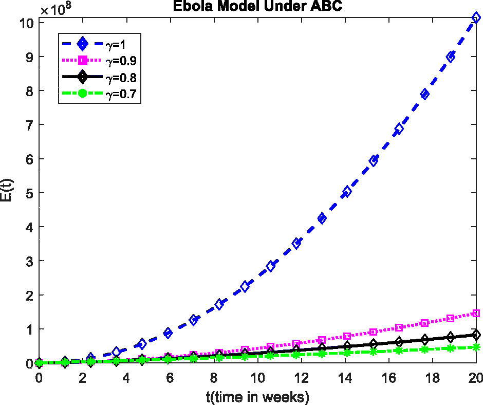

The plot show the dynamics of E(t) in model (1) at various values of fractional order γ.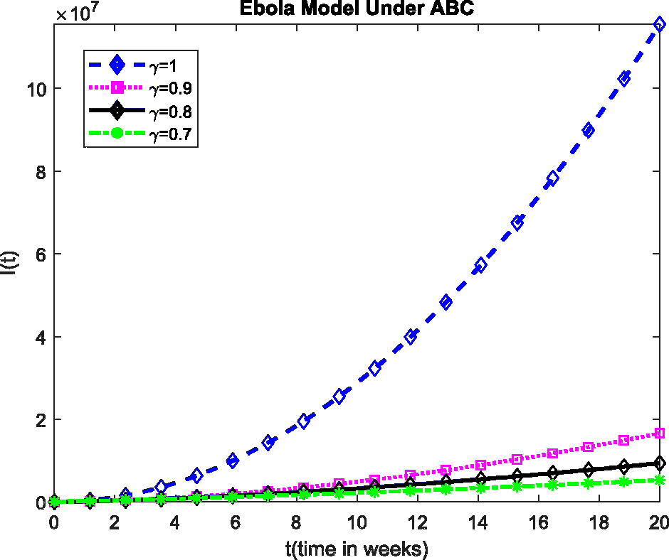

The plot show the dynamics of I(t) in model (1) at various values of fractional order γ.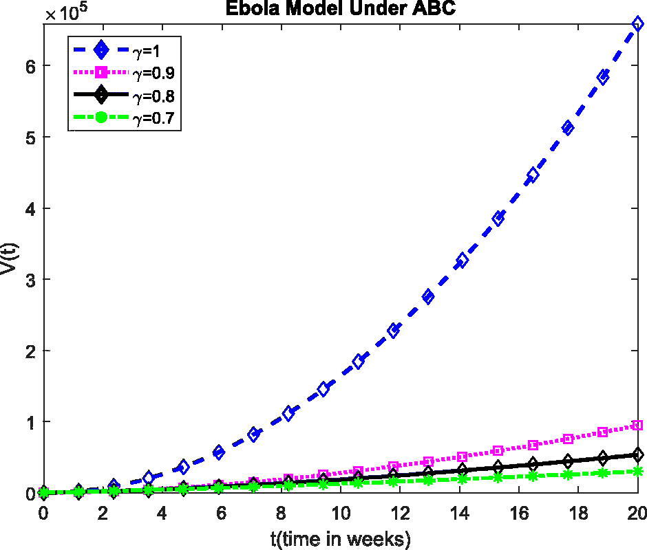

The plot show the dynamics of V(t) in model (1) at various values of fractional order γ.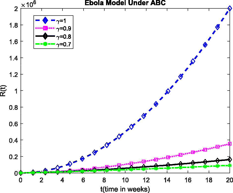

The plot show the dynamics of R(t) in model (1) at various values of fractional order γ. The present investigation may help the researchers to understand some stimulating consequences of the projected model. Also, the fractional operator can exemplify some features of considered model defined in above Figures. From the plots, for the change of value of γ, the obtained solution gives fascinating consequences with a fixed value of the parameters defined in the projected model. These plots show the exponential growth in all the classes which we can be seen from the beginning.

8. Conclusion

We successfully obtained the conditions for the qualitative and approximate solution of Ebole model model under fractional order derivative with out singular kernel of ABC type. With the help of tools of analysis, we proved the existence results of the proposed model. The semi-analytical results are obtained via Laplace Adomian decomposition method. To illustrate the dynamics behaviours of consider model, we also provides graphical presentations.

Acknowledgements

We are thankful to the reviewers for their valuable suggestions and recommendations which has improved this paper very well.

Disclosure statement

There exist no competing interests regarding this research work.

References

- Abassy, T. A., El-Tawil, A. M., & El-Zoheiry, H. (2007). Exact solutions of some nonlinear partial differential equations using the variational iteration method linked with Laplace transforms and the pade technique. Computers & Mathematics with Applications, 54(7-8), 940–954. doi:10.1016/j.camwa.2006.12.067
- Abdilraze, A., & Pelinosky, D. (2009). Convergence of the Adomian Decomposition method for initial value problems. Numerical Methods Partial Differential Equations, 27, 749–766.
- Agarwal, R.P., Belmekki, M., & Benchohra, M. A. (2009). Survey on semilinear differential equations and inclusions involving Riemann-Liouville fractional derivative. Advance Difference Equations, 2009, 47.
- Akram, G., & Tariq, H. (2018). Quintic spline collocation method for fractional boundary value problems. Araba Journal Basic and Applied Science, 23, 57–65.
- Algahtani, O. (2016). Comparing the Atangana-Baleanu and Caputo-Fabrizio derivative with fractional order Allen Cahn model. Chaos, Solitons & Fractals, 89, 552–559. doi:10.1016/j.chaos.2016.03.026
- Ali, A., Samet, B., Shah, K., & Khan, R. A. (2017). Existence and stability of solution to a toppled systems of differential equations of non-integer order. Boundary Value Probems, 2017, 16.
- Ali, A., Shah, K., & Khan, R.A. (2016). Existence of positive solution to a class of boundary value problems of fractional differential equations. Comptational Methods for Differential Equations, 4(1), 19–29.
- Ali, Z., Zada, A., & Shah, K. (2018). Ulam stability to a toppled system of nonlinear implicit fractional order boundary value problem. Boundary Value Problems, 175, 1–16.
- Anjum, N., & He, J. (2019). Laplace transform: Making the variational iteration method easier. Applied Mathematics Letters, 92, 134–138. doi:10.1016/j.aml.2019.01.016
- Anjum, N., Suleman, M., Lu, D., He, J., & Ramzan, M. (2019). Numerical iteration for nonlinear oscillators by Elzaki transform. Journal of Low Frequency Noise, Vibration and Active Control, 1–6. doi:10.1177/1461348419873470.
- Atangana, A., & Baleanu, D. (2016). New fractional derivatives with nonlocal and non-singular kernel. Theory and application to heat transfer model. Thermal Science, 20(2), 763–769. doi:10.2298/TSCI160111018A
- Beauchemin, C. A. A., & Handel, A. (2011). Review of mathematical models of influenza A infections within a host or cell culture: Lessons learned and challenges ahead. BMC Public Health, 11(Suppl 1), S7. doi:10.1186/1471-2458-11-S1-S7
- Benchohra, M., Hamani, S., & Ntouyas, S.K. (2009). Boundary value problems for differential equations with fractional order and nonlocal conditions. Journal of Nonlinear Analysis, 71(7-8), 2391–2396. doi:10.1016/j.na.2009.01.073
- Biazar, J. (2006). Solution of the epidemic model by Adomian decomposition method. Applied Mathematics and Computation, 173(2), 1101–1106. doi:10.1016/j.amc.2005.04.036
- Bowen, E. T., Lloyd, G., Harris, W. J., Platt, G. S., Baskerville, A., & Vella, E. E. (1977). Viral haemorrhagic fever in southern Sudan and northern Zaire. Preliminary studies on the aetiological agent. Lancet, 1(8011), 571–573. doi:10.1016/S0140-6736(77)92001-3
- Brauer, F., Driessche, V. d., & Wu, J. (2008). Lecture notes in mathematical epidemiology. Berlin, Germany. Springer, 75(1), 3–22.
- Cai, L., & Wu, J. (2009). Analysis of an HIV/AIDS treatment model with a nonlinear incidence rate. Chaos, Solitons & Fractals, 41(1), 175–182. doi:10.1016/j.chaos.2007.11.023
- Caputo, M. (1967). Linear Models of dissipation whose Q is almost frequency independent. Geophysical Journal International, 13(5), 529–539. doi:10.1111/j.1365-246X.1967.tb02303.x
- Deghan, M., Yousefi, Y. A., & Lotfi, A. (2011). The use of He’s variational iteration method for solving the telegraph and fractional telegraph equations. International Journal Numerical Methods and Biomedicen Engineering, 2, 219–231.
- Djida, J. D., Atangana, A., & Area, I. (2017). Numerical computation of a fractional derivative with non-local and non-singular kernel. Mathematical Modelling of Natural Phenomena, 12(3), 4–13. doi:10.1051/mmnp/201712302
- Edelstein-Keshet, L. (2005). Mathematical models in biology. Philadelphia: Society for Industrial and Applied Mathematics.
- Hesameddini, E., & Latifizadeh, H. (2009). Reconstruction of variational iteration algorithms using the Laplace transform. International Journal Nonlinear Science and Numerical Simulation, 10(11-12), 1377–1382.
- Hilfer, R. (2000). Applications of fractional calculus in physics. Singapore: World Scientific.
- Hyers, D. H. (1941). On the stability of the linear functional equation. Proceedings of the National Academy of Sciences of the United States of America, 27(4), 222–224. doi:10.1073/pnas.27.4.222
- Khan, R. A., & Shah, K. (2015). Existence and uniqueness of solutions to fractional order multi-point boundary value problems. Communication in Applied Analysis, 19(4), 515–526.
- Kilbas, A. A., Marichev, O. I., & Samko, S. G. (1993). Fractional integrals and derivatives (Theory and applications). Switzerland: Gordon and Breach.
- Kilbas, A. A., Srivastava, H.M., & Trujillo, J.J. (2006). Theory and applications of fractional differential equations (Vol. 13). Amsterdam: Elsevier.
- Kuhn, J. H., Becker, S., Ebihara, H., Geisbert, T. W., Johnson, K. M., Kawaoka, Y., … Jahrling, P. B. (2010). Proposal for a revised taxonomy of the family Filoviridae: Classification, names of taxa and viruses, and virus abbreviations. Archives of Virology, 155(12), 2083–2103. doi:10.1007/s00705-010-0814-x
- Kumar, D., Singh, J., & Kumar, S. (2015). Numerical computation of fractional multi-dimensional diffusion equations by using a modified homotopy perturbation method. Araba Jounrnal of Basic and Applied Science, 17, 20–26.
- Lakshmikantham, V., Leela, S., & Vasundhara, J. (2009). Theory of fractional dynamic systems. Cambridge, UK: Cambridge Academic Publishers.
- Lamb, R. A. (2013). Fields virology (pp. 923–956). Philadelphia, PA: Lippincott Williams and Wilkins.
- Lijun, G., Wang, D., & Wang, G. (2015). Further results on exponential stability for impulsive switched nonlinear time-delay systems with delayed impulse effects. Applied Mathematics and Computation, 268, 186–200.
- Maitama, S., & Zhao, W. (2020). New homotopy analysis transform method for solving multidimensional fractional diffusion equations. Arab Journal of Basic and Applied Sciences, 27(1), 27–44. doi:10.1080/25765299.2019.1706234 Ok
- Miller, K. S., & Ross, B. (1993). An introduction to the fractional calculus and fractional differential equations. New York: Wiley.
- Mokhtari, R., & Mohammadi, M. (2009). Some remarks on the variational iteration method. International Journal of Nonlinear Science and Numerical Simulation, 10, 67–74.
- Murray, J. D. (2007). Mathematical biology: An introduction (Vol. 17). Berlin: Springer Science and Business Media.
- Naghipour, A., & Manafian, J. (2015). Application of the Laplace adomian decomposition method and implicit methods for solving Burger’s equation. TWMS Journal Pure Applied Mathematics, 6(1), 68–77.
- Nanware, A., & Dhaigude, D. B. (2014). Existence and uniqueness of solutions of differential equations of fractional order with integral boundary conditions. Journal of Nonlinear Sciences and Applications, 07(04), 246–254. doi:10.22436/jnsa.007.04.02
- Odibat, Z., & Momani, S. (2008). A generalized differential transform method for linear partial differential equations of fractional order. Applied Mathematics Letters, 21(2), 194–199. doi:10.1016/j.aml.2007.02.022
- Pattyn, S., van der Groen, G., Jacob, W., Piot, P., & Courteille, G. (1977). Isolation of Marburg-like virus from a case of haemorrhagic fever in Zaire. The Lancet, 1(8011), 573–574.
- Podlubny, I. (1999). Fractional differential equations, mathematics in science and engineering. New York: Academic Press.
- Rafei, M., Ganji, D.D., & Daniali, H. (2007). Solution of the epidemic model by homotopy perturbation method. Applied Mathematics and Computation, 187(2), 1056–1062. doi:10.1016/j.amc.2006.09.019
- Rahimkhani, P., Ordokhani, Y., & Babolian, E. (2017). Numerical solution of fractional pantograph differential equations by using generalized fractional-order Bernoulli wavelet. Journal of Computational and Applied Mathematics, 309, 493–510. doi:10.1016/j.cam.2016.06.005
- Rassias, T. M. (1978). On the stability of the linear mapping in Banach spaces. Proceedings of the American Mathematical Socity, 72, 297–300.
- Rvachev, L., Ira, M., & Longini, J. (1985). A mathematical model for the global spread of influenza. Mathematical Biosciences, 75(1), 3–22. doi:10.1016/0025-5564(85)90064-1
- Saeed, U., & Rehman, M. (2014). Hermite wavelet method for fractional delay differential equations. Journal of Difference Equations, 2014, 1–8. doi:10.1155/2014/359093
- Shah, K., Alqudah, M. A., Jarad, F., & Abdelijawad, T. (2020). Semi-analytical study of Pine Wilt Disease model with convex rate under Caputo-Fabrizio fractional order derivative. Chaos, Solitons & Fractals,135, 109754.
- Shah, K., & Khan, R. A. (2015). Existence and uniqueness of positive solutions to a coupled system of nonlinear fractional order differential equations with anti periodic boundary conditions. Differential Equatrions and Applications, 7(2), 245–262.
- Shah, K., Khalil, H., & Khan, R. A. (2018). Analytical solutions of fractional order diffusion equations by Natural transform method. Iranian Journal of Science and Technology, Transactions A: Science, 42(3), 1479–1490. doi:10.1007/s40995-016-0136-2
- Stamova, I. (2015). Mittag-Leffler stability of impulsive differential equations of fractional order. Journal of Applied Mathematics, 73(3), 525–535.
- Suleman, M., Lu, D., Yue, C., Ul Rahman, J., & Anjum, N. (2019). He Laplace method for general nonlinear periodic solitary solution of vibration equations. Journal of Low Frequency Noise, Vibration and Active Control, 38(3-4), 1297–1304. doi:10.1177/1461348418816266
- Tahir, M., Shah, S. I. A., Zaman, G., & Khan, T. (2019). A dynamic compartmental mathematical model describing the transmissibility of MERS-CoV virus in public. Journal of Mathematics, 51(4), 57–71.
- Trigeassou, J.C., Maamri, N., Sabatier, J., & Oustaloup, A. (2011). A Lyapunov approach to the stability of fractional differential equations. Signal Processing, 91(3), 437–445. doi:10.1016/j.sigpro.2010.04.024
- Ullam, S. M. (1940). Problems in modern mathematics. Science Editors. New York: Wiley.
- Ulam, S. M. (1960). A collection of mathematical problems. New York: Interscience.
- Wu, R.C., Hei, X.D., & Chen, L.P. (2013). Finite-time stability and finite-time bounbednees of fractional-order linear systems. Communications in Theoretical Physics, 60(2), 189–193. doi:10.1088/0253-6102/60/2/08
- Yang, S., Xiao, A., & Su, H. (2010). Convergence of the variational iteration method for solving multi-order fractional differential equations. Computers & Mathematics with Applications, 60(10), 2871–2879. doi:10.1016/j.camwa.2010.09.044
- Yang, Y., & Huang, Y. (2013). Spectral-collocation methods for fractional pantograph delay integrodifferential equations. Advances in Mathematical Physics, 2013, 1–14. doi:10.1155/2013/821327
- Zhou, P., Yang, X.-L., Wang, X.-G., Hu, B., Zhang, L., Zhang, W., … Shi, Z.-L. (2020). A pneumonia outbreak associated with a new coronavirus of probable bat origin. Nature, 579(7798), 270–273. doi:10.1038/s41586-020-2012-7
- Zhou, Y. (2016). Basic theory of fractional differential equations. Singapore: World Scientific Publishing.