Reproducing kernel method for the solutions of non-linear partial differential equations

Abstract

In modeling of a lots of complex physical problems and engineering process, the non-linear partial differential equations have a very important role. Development of dependable and effective methods to solve such types equations are constructed. In the suggested technique, reproducing kernel method is examined to approximate the solutions together with reproducing kernel functions. In order to demonstrate accuracy, the performance and reliability of the proposed method, the results of the experiments and the available results are compared. There is high stability for a higher degree of accuracy between the solutions.

Keywords:

• Reproducing kernel functions
• bounded linear operator
• Hilbert spaces
• partial differential equations

2000 MATHEMATICS SUBJECT CLASSIFICATION:

• 47B32
• 46E22
• 34A12
• 49K20

1. Introduction

For a large number of problems in science and engineering, it is important to explain their structures and their effects on environment and humans. For this reason, many mathematical models were derived. To understand and define the physics of the complicated problems, nonlinear partial differential equations (NPDEs) were essentially used.

Burgers’ equation, which has important position in NPDEs, was first introduced by Bateman in 1915 and later analyzed by Dutch physicist J.H. Burgers in 1948. This equation was originally used to explain the nature of turbulence, acoustic transmission, traffic flow etc. Afterwards, it was used in different fields like fluid mechanics, gas dynamics as a fundamental NPDE. On the other hand, Fisher proposed a model in 1937 which is used to model heat and reaction-diffusion problems. Later, several applications were also provided in many other fields such as mathematical biology, chemistry, genetics, engineering and neurophysiology. Another important equation which has significant applications in several fields is Huxley equation. It is a nonlinear model and also it was showed up in biology, fluid dynamics and so on. Additionally, combined form of these equations are quite fundamental to explain wide variety of problems in several fields.

Many powerful techniques were introduced to get solutions of the NPDEs, including a new integral transform, Backlund transformation and Hopf-Cole transformation (Aronson & Weinberger, 1988; Babolian & Saeidian, 2009; Olmos & Shizgal, 2006). Under some common assumptions, the longitudinal dispersion problem was investigated by Ebach and White Ebach and White, Ebach and White, (1958). Joshi et al. (Benton & Platzman, 1972; Kutluay et al., 1999, 2004; Xu & Xian, 2010) utilized theoretical technique for the solution of Burgers’ equation, and he was followed by many other scholars. Moreover, due to various applications of Fisher equation, Burgers’ equation, Huxley equation and Burgers-Fisher equation in several fields, solutions of these equations were provided by many authors as well (Babolian & Saeidian, 2009; Jaiswal et al., 2019; Kaya & El-Sayed, 2003; Wazwaz, 2008).

There is no doubt that various efficient methods have been proposed to get the solutions of these NPDEs since the past half-century. In this article, the main aim is to find the approximate solutions of the mentioned NPDEs with some examples by using the advantages of reproducing kernel method (RKM). This method is pretty powerful and has many virtues. For instance, it is precise and requires less exertion to discover the numerical results. Also, it avoids massive computational prerequisites and it is easily applied and capable in treating various boundary conditions. Thus, the approximate solutions can be obtained in a shorter time by applying the RKM.

The reproducing kernel method was first used in the early 20th century in Zaremba’s work. It was on boundary value problems for harmonic and two harmonic moduli. After some years, the idea of reproducing kernel was restored by three mathematicians from Germany named Zigo (1921), Bergman (1922) and Bacchner (1922). The general theory of the RKM was established by Aronszajn and Bergman in 1950. Javan et al. Javan et al., Javan et al., (2017) have proposed an application of the RKM for investigating a class of nonlinear integral equations. Sakar Sakar, Sakar, (2017) has implemented the method to Riccati differential equation. The reproducing kernel method was applied by many authors to obtain several scientific applications. Toutian Isfahani et al. Toutian Isfahani et al., (2020) have obtained the numerical solution of some initial optimal control problems using the reproducing kernel Hilbert space technique. Zhao et al. Zhao et al., Zhao et al., (2016) have investigated the convergence order of the reproducing kernel method for solving boundary value problems. Sahihi et al. Sahihi et al., Sahihi et al., (2020) have studied on solving system of second-order BVPs using a new algorithm based on reproducing kernel Hilbert space. For interesting results and more details about this method, we refer the reader to (Bergman, 1950; Beyrami et al., 2017; Foroutan et al., 2018; Zaremba, 1907, 1908) and the references cited therein.

We organize our manuscript as: We discuss the applications of the reproducing kernel method in Section 2. We construct the reproducing kernel Hilbert spaces in this section. We obtain very useful reproducing kernel functions in these spaces. We demonstrate the numerical results in Section 3. We give the conclusion in the last section.

2. Application of the reproducing kernel method

We construct the following reproducing kernel Hilbert spaces. Then, we obtain the reproducing kernel functions in these spaces. We use these reproducing kernel functions to obtain the numerical results of the problems by the reproducing kernel method.

2.1. Reproducing kernel functions

Definition 2.1.

We describe the reproducing kernel space $V_2^1[0,1]$ by: $$V_2^1[0,1]=\{\zeta \in AC[0,1]:\zeta \prime \in L^2[0,1\left]\right\}.$$

We describe the inner product of this space by: $${〈\zeta ,\gamma 〉}_{V_2^1}=\zeta (0)\gamma (0)+{\int }_0^1\zeta \prime (\theta )\gamma \prime (\theta )d\theta .$$

We obtain the reproducing kernel function m_t by: (2.1) $$m_t(\theta )=\{\begin{array}{l}1+\theta ,\hspace{1em}0\le \theta \le t\le 1,\hfill \\ 1+t,\hspace{1em}0\le t<\theta \le 1.\hfill \end{array}$$(2.1)

Definition 2.2.

We describe the reproducing kernel space $V_2^2[0,1]$ by: $$V_2^2[0,1]=\{\zeta \in AC[0,1]:{\zeta }^{\prime }\in AC[0,1],\zeta ″\in L^2[0,1\left]\right\}.$$

We describe the inner product and the norm as: $${〈\zeta ,\gamma 〉}_{V_2^2[0,1]}=\zeta (0)\gamma (0)+\zeta \prime (0)\gamma \prime (0)+{\int }_0^1\zeta ″(\theta )\gamma ″(\theta )\mathrm{d}\theta ,\hspace{1em}\zeta ,y\in V_2^2[0,1],$$ and $$\left|\right|\zeta {\Vert }_{V_2^2[0,1]}=\sqrt{{〈\zeta ,\zeta 〉}_{V_2^2[0,1]}},\hspace{1em}\zeta \in V_2^2[0,1].$$

We obtain the reproducing kernel function M_x as: (2.2) $$M_x(\theta )=\{\begin{array}{c}1+\theta x+\frac{1}{2}x{\theta }^2-\frac{{\theta }^3}{6},\hspace{1em}0\le \beta \le x\le 0,\hfill \\ \hfill \\ 1+\theta x+\frac{1}{2}{x}^2\theta -\frac{x^3}{6},\hspace{1em}0\le x<\theta \le 1.\hfill \end{array}$$(2.2)

Definition 2.3.

We describe the reproducing kernel space ${}^0{V}_2^2[0,1]$ by: $${}^0{V}_2^2[0,1]=\{\zeta \in AC[0,1]:{\zeta }^{\prime }\in AC[0,1],\zeta ″\in L^2[0,1],\zeta (0)=0\}.$$

We give the inner product and the norm as: $${〈\zeta ,\gamma 〉}_{{}^0{V}_2^2[0,1]}=\zeta (0)\gamma (0)+\zeta \prime (0)\gamma \prime (0)+{\int }_0^1\zeta ″(\beta )\gamma ″(\beta )\mathrm{d}\beta ,\hspace{1em}\zeta ,\gamma \in {}^0{V}_2^2[0,1],$$ and $${\Vert \zeta \Vert }_{{}^0{V}_2^2[0,1]}=\sqrt{{〈\zeta ,\zeta 〉}_{{}^0{V}_2^2[0,1]}},\hspace{1em}\zeta {\in }^0{V}_2^2[0,1].$$

We obtain the kernel function as: (2.3) $$N_x(\beta )=\{\begin{array}{c}\beta x+\frac{1}{2}x{\beta }^2-\frac{{\beta }^3}{6},\hspace{1em}0\le \beta \le x\le 0,\hfill \\ \hfill \\ \beta x+\frac{1}{2}{x}^2\beta -\frac{x^3}{6},\hspace{1em}0\le x<\beta \le 1.\hfill \end{array}$$(2.3)

Definition 2.4.

We present the reproducing kernel space ${}^0{V}_2^3[0,1]$ by: $${}^0{V}_2^3[0,1]=\{r\in AC[0,1]:r\prime ,r″\in AC[0,1],r^{(3)}\in L^2[0,1],r(0)=0=r(1)\}.$$ We construct the inner product and the norm as: $${〈r,p〉}_{V_2^3}=\sum _{i=0}^2{r}^{(i)}(0)p^{(i)}(0)+{\int }_0^1{r}^{(3)}(t)p^{(3)}(t)\mathrm{d}t,\hspace{1em}r,p\in V_2^3[0,1]$$ and $${\Vert r\Vert }_{V_2^3}=\sqrt{{〈r,r〉}_{{}^0{V}_2^3}},\hspace{1em}r\in V_2^3[0,1].$$

Reproducing kernel function of ${}^0{V}_2^3[0,1]$ can be found in a similar way.

Definition 2.5.

For $k+l>2,$ we construct the binary space (Olmos & Shizgal, 2006): $$V_2^{(k,l)}(\Omega )=\{u:\Omega \to \mathbb{R}\hspace{0.17em}|\hspace{0.17em}Du\in V_2^{(1,1)}(\Omega )\hspace{0.17em}\text{ if signature}(D)(k-1,l-1)\}.$$

If equipped with the inner product $$\begin{array}{c}{〈r,p〉}_{V_2^{(k,l)}(\Omega )}=\sum _{i=0}^{k-1}{\int }_0^1\frac{{\partial }^n}{\partial t^l}\frac{{\partial }^{i}r}{\partial x^i}(0,t)\frac{{\partial }^l}{\partial t^l}\frac{{\partial }^{i}p}{\partial x^i}(0,t)dt\\ \hspace{1em}+\sum _{j=0}^{l-1}{〈\frac{{\partial }^{j}r}{\partial t^j}(·,0),\frac{{\partial }^{j}p}{\partial t^j}(·,0)〉}_{V_2^k[0,1]}\\ +{\iint }_{\Omega }\frac{{\partial }^2}{\partial x\partial t}\left(\frac{{\partial }^{k+l-2}h}{\partial x^{k-1}\partial t^{l-1}}\right)(x,t)\frac{{\partial }^2}{\partial x\partial t}\left(\frac{{\partial }^{k+l-2}p}{\partial x^{k-1}\partial t^{l-1}}\right)(x,t)\mathit{dxdt}\end{array}$$ then $V_2^{(k,l)}(\Omega )$ is a RKHS.

The reproducing kernel method is implemented to investigate the following problem: (2.4) $$\frac{\partial v(y,\tau )}{\partial \tau }=\gamma (y,\tau )\frac{{\partial }^2}{\partial y^2}v(y,\tau )+\frac{\partial }{\partial y}\xi (v)+\zeta (v),\hspace{1em}a<y<b,\tau >0$$(2.4) or (2.5) $$v_{\tau }=\gamma v_{yy}+{(\xi (v))}_y+\zeta (v),\hspace{1em}a<y<b,\tau >0,$$(2.5) (2.6) $$v(a,\tau )=f(\tau ),\hspace{1em}\tau >0$$(2.6) (2.7) $$v(b,\tau )=g(\tau ),\hspace{1em}\tau >0,$$(2.7) (2.8) $$v(y,0)=m(y),\hspace{1em}a<y<b,$$(2.8) where γ is diffusivity, $\xi (v)$ and $\zeta (v)$ are nonlinear functions of v. We can write the problem as: (2.9) $$v_{\tau }=\gamma v_{yy}+{(\xi (v))}_y+\zeta (v)+v(y,0)-m(y),\hspace{1em}a<y<b,\hspace{1em}\tau >0.$$(2.9)

We need to homogenize the initial and boundary conditions to apply the reproducing kernel method. Therefore, we use the following transformation. (2.10) $$v(y,\tau )=h(y,\tau )+b(y,\tau )$$(2.10)

Then we reach (2.11) $$h_{\tau }=\gamma h_{yy}+{(\xi (h+b))}_y+\zeta (h+b)-b(y,\tau )+b_{yy}(y,\tau ),\hspace{1em}a<y<b,\tau >0,$$(2.11) (2.12) $$h(a,\tau )=0,\hspace{1em}\tau >0$$(2.12) (2.13) $$h(b,\tau )=0,\hspace{1em}\tau >0,$$(2.13) (2.14) $$h(y,0)=0,\hspace{1em}a<y<b,$$(2.14)

We denote ${(\xi (h+b))}_y+\zeta (h+b)-b(y,\tau )+b_{yy}(y,\tau )$ by $S(h,y,\tau ).$ We will explain the $b(y,\tau )$ in details in the next section for different examples.

Because of the structure of the problem (2.4)(2.4) $$\frac{\partial v(y,\tau )}{\partial \tau }=\gamma (y,\tau )\frac{{\partial }^2}{\partial y^2}v(y,\tau )+\frac{\partial }{\partial y}\xi (v)+\zeta (v),\hspace{1em}a<y<b,\tau >0$$(2.4) , we will be obtain the solution in the reproducing kernel Hilbert space ${}^0{V}_2^{(3,2)}(\Omega )$ which is a binary space. Let us define the bounded linear operator as $$\begin{array}{c}\mathbb{L}:{}^0{V}_2^{(3,2)}(\Omega ){\to }^0{V}_2^{(2,1)}(\Omega )\\ \mathbb{L}h=S(h_k,y_k,{\tau }_k)\end{array}$$ Consider a countable dense subset $\{(y_1,{\tau }_1),(y_2,{\tau }_2),\dots \}$ in Ω and define $${\varrho }_i=E_{(y_i,{\tau }_i)},\hspace{1em}{\vartheta }_i=L^{\ast }{\varrho }_i,$$ where $L^{\ast }$ is the adjoint operator of L and $E_{(y_i,{\tau }_i)}$ is the reproducing kernel function of $V_2^{(2,1)}(\Omega ).$ The orthonormal system ${\left\{{\widehat{\vartheta }}_i\right\}}_{i=1}^{\infty }$ of ${}^0{V}_2^{(3,2)}(\Omega )$ can be obtained by the operation of Gram–Schmidt orthogonalization of ${\left\{{\vartheta }_i\right\}}_{i=1}^{\infty }$ as: $${\widehat{\vartheta }}_i=\sum _{k=1}^i{\beta }_{ik}{\vartheta }_k$$ where β_ik denotes orthogonalization coefficients.

Theorem 2.6.

If ${\{(y_i,{\tau }_i)\}}_{i=1}^{\infty }$ is dense in Ω, then the solution of the problem has been found by reproducing kernel method as: (2.15) $$h=\sum _{i=1}^{\infty }\sum _{k=1}^i{\beta }_{ik}S(h_k,y_k,{\tau }_k){\widehat{\vartheta }}_i.$$(2.15)

Proof.

Let h be the solution of the problem. We know that ${\left\{{\vartheta }_i\right\}}_{i=1}^{\infty }$ is a complete system in ${}^0{V}_2^{(3,2)}(\Omega ).$ Therefore, we get: $$h\mathrm{ }=\sum _{i=1}^{\infty }{〈h,{\widehat{\vartheta }}_i〉}_{{}^0{V}_2^{(3,2)}(\Omega )}{\widehat{\vartheta }}_i=\sum _{i=1}^{\infty }\sum _{k=1}^i{\beta }_{ik}{〈h,{\vartheta }_k〉}_{{}^0{V}_2^{(3,2)}(\Omega )}{\widehat{\vartheta }}_i.$$

We apply the feature of the adjoint operator $L^{\ast }$ and reach: $$h=\sum _{i=1}^{\infty }\sum _{k=1}^i{\beta }_{ik}{〈h,L^{\ast }{\varrho }_k〉}_{{}^0{V}_2^{(3,2)}(\Omega )}{\widehat{\vartheta }}_i=\sum _{i=1}^{\infty }\sum _{k=1}^i{\beta }_{ik}{〈Lh,{\varrho }_k〉}_{V_2^{(2,1)}(\Omega )}{\widehat{\vartheta }}_i.$$ We implement the reproducing feature and obtain: $$h=\sum _{i=1}^{\infty }\sum _{k=1}^i{\beta }_{ik}{〈Lh,E_{(y_k,{\tau }_k)}〉}_{V_2^{(2,1)}(\Omega )}{\widehat{\vartheta }}_i=\sum _{i=1}^{\infty }\sum _{k=1}^i{\beta }_{ik}Lh(y_k,{\tau }_k){\widehat{\vartheta }}_i.$$ Then, we get the desired result as: $$h=\sum _{i=1}^{\infty }\sum _{k=1}^i{\beta }_{ik}S(h_k,y_k,{\tau }_k){\widehat{\vartheta }}_i.$$

The approximate solution h_n can be found as: (2.16) $$h_n=\sum _{i=1}^n\sum _{k=1}^i{\beta }_{ik}S(h_k,y_k,{\tau }_k){\widehat{\vartheta }}_i.$$(2.16)

3. Illustrative examples

To illustrate the efficiency and precision of the suggested approach, some significant nonlinear models have been investigated and the results are compared with the exact solutions which are already exist in literature.

Example 3.1.

Let us consider the following equation (Jaiswal et al., 2019) $$w_t=w_{xx}-w{w}_x,\hspace{1em}0<x<1,\hspace{1em}t>0,$$ which named Burgers equation. The boundary and initial conditions are given as: $$\begin{array}{c}\begin{array}{c}w(0,t)=\frac{1}{2}-\frac{1}{2}\tanh \left(-\frac{1}{8}t\right)\hfill \\ \hfill \\ w(1,t)=\frac{1}{2}-\frac{1}{2}\tanh \frac{1}{4}\left(1-\frac{1}{2}t\right)\hfill \end{array}\begin{array}{c},t>0,\end{array}\\ w(x,0)=\frac{1}{2}-\frac{1}{2}\tanh \left(\frac{x}{4}\right),\hspace{1em}0<x<1.\end{array}$$ $w(x,t)=\frac{1}{2}-\frac{1}{2}\tanh \frac{1}{4}(x-\frac{1}{2}t)$ is the exact solution of the problem.

In order to homogenize the conditions of the given problem, we present the following transformation function: $$\begin{array}{c}b(x,t)=\frac{1}{2}+\frac{1}{2}\tanh \left(\frac{1}{8}t\right)-\frac{1}{2}x\tanh \left(\frac{1}{8}t\right)+\frac{1}{2}x\tanh \left(-\frac{1}{4}+\frac{1}{8}t\right)-\frac{1}{2}\tanh \left(\frac{1}{4}x\right)\\ +\frac{1}{2}x\tanh \left(\frac{1}{4}\right)\end{array}$$

If we apply the boundary and initial conditions to the function b(x, t) and calculate required derivatives we obtain the following equations: $$\begin{array}{c}b(0,t)=\frac{1}{2}+\frac{1}{2}\tanh \left(\frac{t}{8}\right)\\ b(1,t)=\frac{1}{2}+\frac{1}{2}\tanh \left(-\frac{1}{4}+\frac{t}{8}\right)\\ b(x,0)=\frac{1}{2}-\frac{1}{2}\tanh \left(\frac{x}{4}\right)\\ w_t(x,t)=v_t(x,t)+b_t(x,t)\\ =v_t(x,t)+\frac{1}{16}-\frac{1}{16}\tanh {\left(\frac{1}{8}t\right)}^2-\frac{1}{2}x\left(\frac{1}{8}-\frac{1}{8}\tanh {\left(\frac{1}{8}t\right)}^2\right)\\ +\frac{1}{2}x\left(\frac{1}{8}-\frac{1}{8}\tanh {\left(-\frac{1}{4}+\frac{1}{8}t\right)}^2\right)\\ w_x(x,t)=v_x(x,t)-b_x(x,t)\\ =v_x(x,t)-\frac{1}{2}\tanh \left(\frac{1}{8}t\right)+\frac{1}{2}\tanh \left(-\frac{1}{4}+\frac{1}{8}t\right)-\frac{1}{8}\\ +\frac{1}{8}\tanh {\left(\frac{1}{4}x\right)}^2+\frac{1}{2}\tanh \left(\frac{1}{4}\right)\\ w_{xx}(x,t)=v_{xx}(x,t)-b_{xx}(x,t)\\ =v_{xx}(x,t)+\frac{1}{4}\tanh \left(\frac{1}{4}x\right)\left(\frac{1}{4}-\frac{1}{4}\tanh {\left(\frac{1}{4}x\right)}^2\right)\\ w_t=w_{xx}-w{w}_x\\ v_t-b_t=v_{xx}-b_{xx}-(v-b)(v_x-b_x)\\ =v_{xx}-b_{xx}-v{v}_x+b_{x}v+b{v}_x-b{b}_x\\ v_{xx}+b{v}_x-v_t+b_{x}v=-b_t+b_{xx}+v{v}_x+b{b}_x\\ =v{v}_x+b{b}_x-b_t\\ v(0,t)=v(1,t)=v(x,0)=0.\end{array}$$ In Table 1, the Absolute Errors and Relative Errors results are presented. Additionally, we give the absolute errors by Figure 1.

Figure 1. Absolute Errors of Example 3.1.

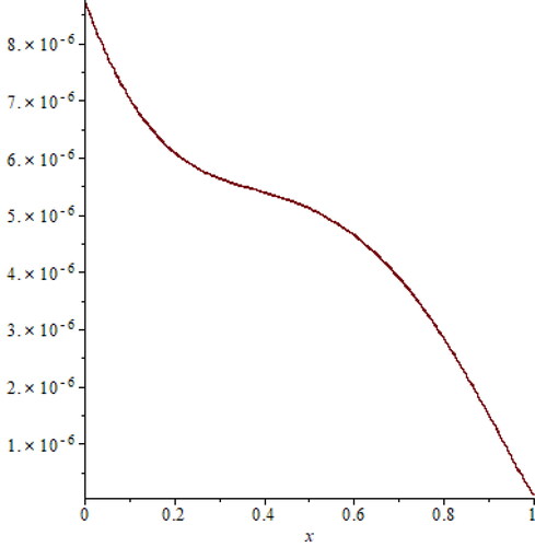
Table 1. Absolute Errors (AE) and Relative Errors (RE) for Example 3.1.

x	(Jaiswal et al., 2019) AE	RKM (AE)	RKM (RE)
0.1	0.0007420	0.0000070399	0.00001280368263
0.2	0.0009930	0.0000060906	0.00001133282800
0.3	0.0008750	0.0000056377	0.00001073890191
0.4	0.0005110	0.0000053926	0.00001052219979
0.5	0.0000527	0.0000051153	0.00001023060000
0.6	0.0004670	0.0000046467	0.00000953164140
0.7	0.0008370	0.0000039009	0.00000821206123
0.8	0.0009640	0.0000028419	0.00000614371673
0.9	0.0007250	0.0000014981	0.00000332788347

Example 3.2.

Consider the Fisher equation (Jaiswal et al., 2019) $$w_t=w_{xx}+w(1-w),\hspace{1em}0<x<1,\hspace{1em}t>0,$$ with the boundary and initial conditions $$\begin{array}{c}\begin{array}{c}w(0,t)=\frac{1}{4}{[1-\tanh (-\frac{5}{12}t\left)\right]}^2,\hfill \\ \hfill \\ w(1,t)=\frac{1}{4}{[1-\tanh (\frac{1}{2\sqrt{6}}(1-\frac{5}{\sqrt{6}}t)\left)\right]}^2,\hfill \end{array}\begin{array}{c},t>0,\end{array}\\ w(x,0)=\frac{1}{4}{[1-\tanh (\frac{x}{2\sqrt{6}}\left)\right]}^2,\hspace{1em}0<x<1.\end{array}$$ The exact solution is given as $w(x,t)=\frac{1}{4}{[1-\tanh (\frac{1}{2\sqrt{6}}(x-\frac{5}{\sqrt{6}}t))]}^2.$ In order to homogenize the conditions, we use the following transformation, $$\begin{array}{cc}b(x,t)\hfill & =\frac{1}{4}{\left[1+\tanh \left(\frac{5}{12}t\right)\right]}^2(1-x)+\frac{1}{4}x{\left[1-\tanh \left(\frac{\sqrt{6}}{12}\left(1-\frac{5}{6}t\sqrt{6}\right)\right)\right]}^2\hfill \\ \hfill & \hspace{1em}+\frac{1}{4}{\left[1-\tanh \left(\frac{1}{12}x\sqrt{6}\right)\right]}^2-\frac{1}{4}x{\left[1-\tanh \left(\frac{1}{12}\sqrt{6}\right)\right]}^2-\frac{1}{4}+\frac{1}{4}x.\hfill \end{array}$$ In Table 2 the Absolute Errors and Relative Errors are presented.

Table 2. Absolute Errors (AE) and Relative Errors (RE) for Example 3.2.

x	(Jaiswal et al., 2019) AE	RKM (AE)	RKM (RE)
0.1	0.000893000	0.0000122759	0.00002590656598
0.2	0.001170000	0.0000274022	0.00005934011860
0.3	0.001020000	0.0000396663	0.00008820767473
0.4	0.000581000	0.0000478987	0.00010945859770
0.5	0.000000650	0.0000508509	0.00011950619050
0.6	0.000593000	0.0000487675	0.00011795494960
0.7	0.001030000	0.0000418720	0.00010431231750
0.8	0.001180000	0.0000306639	0.00007874111457
0.9	0.000891000	0.0000162273	0.00004298553455

Example 3.3.

We take into consideration the Huxley equation (Jaiswal et al., 2019) $$w_t=w_{xx}+w(1-w)(w-1),\hspace{1em}0<x<1,t>0,$$ with boundary and initial conditions $$\begin{array}{c}\begin{array}{c}w(0,t)=\frac{1}{2}+\frac{1}{2}\tanh (-\frac{1}{4}t),\hfill \\ \hfill \\ w(1,t)=\frac{1}{2}+\frac{1}{2}\tanh \left(\frac{1}{2\sqrt{2}}\right(1-\frac{1}{\sqrt{2}}t\left)\right),\hfill \end{array}\begin{array}{c}t>0,\end{array}\\ w(x,0)=\frac{1}{2}+\frac{1}{2}\tanh \left(\frac{x}{2\sqrt{2}}\right),\hspace{1em}0<x<1.\end{array}$$ The exact solution is given as $w(x,t)=\frac{1}{2}+\frac{1}{2}\tanh \left(\frac{1}{2\sqrt{2}}\right(x-\frac{1}{\sqrt{2}}t\left)\right).$ To homogenize the conditions, we use the following transformation, $$\begin{array}{c}c(x,t)=\frac{1}{2}-\frac{1}{2}\tanh \left(\frac{1}{4}t\right)(1-x)+\frac{1}{2}x\mathrm{\hspace{0.17em}tanh}\left(\frac{1}{4}\sqrt{2}\left(1-\frac{1}{2}t\sqrt{2}\right)\right)\\ +\frac{1}{2}\tanh \left(\frac{1}{4}\sqrt{2}x\right)-\frac{1}{2}x\mathrm{\hspace{0.17em}tanh}\left(\frac{1}{4}\sqrt{2}\right).\end{array}$$ In Table 3 the Absolute Errors and Relative Errors are demonstrated.

Table 3. Absolute Errors (AE) and Relative Errors (RE) for Example 3.3.

x	(Jaiswal et al., 2019) AE	RKM (AE)	RKM (RE)
0.1	0.001160000	0.0007465299	0.001893323314
0.2	0.001570000	0.0013984488	0.003400039603
0.3	0.001410000	0.0019481619	0.004546194011
0.4	0.000879000	0.0023744036	0.005324693916
0.5	0.000146000	0.0026380162	0.005692082161
0.6	0.000598000	0.0026837855	0.005578725047
0.7	0.001160000	0.0024778811	0.004968245519
0.8	0.001380000	0.0019829011	0.003839740044
0.9	0.001050000	0.0011654422	0.002182286983

Example 3.4.

We take into consideration $$w_t=w_{xx}+w_x+w(1-w),\hspace{1em}0<x<1,t>0,$$ with boundary and initial conditions $$\begin{array}{c}\begin{array}{c}w(0,t)=\frac{1}{2}+\frac{1}{2}\tanh \left(\frac{5}{8}t\right),\hfill \\ \hfill \\ w(1,t)=\frac{1}{2}+\frac{1}{2}\tanh (\frac{1}{4}(1+\frac{5}{\sqrt{2}}t),\hfill \end{array}\begin{array}{c}t>0,\end{array}\\ w(x,0)=\frac{1}{2}+\frac{1}{2}\tanh \left(\frac{x}{4}\right),\hspace{1em}0<x<1.\end{array}$$ The exact solution is given by $w(x,t)=\frac{1}{2}+\frac{1}{2}\tanh (\frac{1}{4}(x+\frac{5}{2}t)).$ We utilize the following transformation to homogenize the conditions. $$d(x,t)=\frac{1}{2}+\frac{1}{2}\tanh \left(\frac{5}{8}t\right)(1-x)+\frac{1}{2}\tanh \left(\frac{1}{4}+\frac{5}{8}t\right)x+\frac{1}{2}\tanh \left(\frac{1}{4}x\right)-\frac{1}{2}\tanh \left(\frac{1}{4}\right)x.$$ In Table 4 the Absolute Errors and Relative Errors are demonstrated.

Table 4. Absolute Errors (AE) and Relative Errors (RE) for Example 3.4.

x	(Jaiswal et al., 2019) AE	RKM (AE)	RKM (RE)
0.1	0.000143000	0.0000640847	0.0000815498182
0.2	0.000194000	0.0001337069	0.0001683691116
0.3	0.000088500	0.0001942380	0.0002421365011
0.4	0.000021300	0.0002369601	0.0002925438989
0.5	0.000012100	0.0002559659	0.0003130796123
0.6	0.000573000	0.0002482271	0.0003009127990
0.7	0.000712000	0.0002137537	0.0002569098277
0.8	0.000813000	0.0001558129	0.0001857367532
0.9	0.000051500	0.0000811149	0.0000959332557

Example 3.5.

$$w_t=w_{xx}+w{w}_x+w(1-w)(w-1),\hspace{1em}0<x<1,t>0,$$ with boundary conditions $$\begin{array}{c}w(0,t)=\frac{1}{2}-\frac{1}{2}\tanh \left(\frac{3}{8}t\right),\hfill \\ \hfill \\ w(1,t)=\frac{1}{2}-\frac{1}{2}\tanh (\frac{1}{4}(1+\frac{3}{2}t),\hfill \end{array}\begin{array}{c}t>0,\end{array}$$ and the initial condition $$w(x,0)=\frac{1}{2}-\frac{1}{2}\tanh \left(\frac{x}{4}\right),\hspace{1em}0<x<1.$$ The exact solution of this problem is presented as $w(x,t)=\frac{1}{2}-\frac{1}{2}\tanh [\frac{1}{4}(x+\frac{3}{2}t)].$

We use the following transformation to homogenize the conditions. $$e(x,t)=\frac{1}{2}-\frac{1}{2}\tanh \left(\frac{3}{8}t\right)\left(1-x\right)-\frac{1}{2}\tanh \left(\frac{1}{4}+\frac{3}{8}t\right)x.$$ In Table 5 the Absolute Errors and Relative Errors are presented.

Table 5. Absolute Errors (AE) and Relative Errors (RE) for Example 3.5.

x	(Jaiswal et al., 2019) AE	RKM (AE)	RKM (RE)
0.1	0.000383000	0.0000852366	0.0002749341420
0.2	0.000476000	0.0001286743	0.0004297267208
0.3	0.000342000	0.0001267512	0.0004385088458
0.4	0.000063200	0.0000893684	0.0003204491351
0.5	0.000277000	0.0000358717	0.0001333810903
0.6	0.000597000	0.0000084603	0.0000326368857
0.7	0.000813000	0.0000335242	0.0001342364626
0.8	0.000084300	0.0000380001	0.0001580117464
0.9	0.000060500	0.0000245051	0.0001058648972

4. Conclusions

In the present paper, the reproducing kernel Hilbert space method was presented to investigate nonlinear partial differential equations with some initial and boundary conditions. The numerical results were showed by some tables. The accuracy of the method was proved theoretically.

Disclosure statement

No potential conflict of interest was reported by the authors.

References

- Al-Khaled, K. (2001). Numerical study of fisher’s reaction diffusion equation by the sine collocation method. The Journal of Computational and Applied Mathematics, 137(2), 245–255. doi:https://doi.org/10.1016/S0377-0427(01)00356-9
- Aronson, D. G., & Weinberger, H. F. (1988). Nonlinear diffusion in population genetics combustion and never pulse propagation. New York, NY: Springer- Verlag.
- Babolian, E., & Saeidian, J. (2009). Analytic approximate solutions to burgers, fisher, huxley equations and two combined forms of these equations. Communications in Nonlinear Science and Numerical Simulation, 14(5), 1984–1992.
- Batiha, B., Noorani, M. S. M., & Hashim, I. (2007). Numerical simulation of the generalized huxley equation by he’s variational iteration method. Journal of Applied Mathematics and Computing, 186, 1322–1325.
- Batiha, B., Noorani, M. S. M., & Hashim, I. (2008). Application of variational iteration method to the generalized burgers-huxley equation. Chaos, Solitons & Fractals, 36(3), 660–663. doi:https://doi.org/10.1016/j.chaos.2006.06.080
- Benton, E., & Platzman, G. W. (1972). A table of the solutions of the one dimensional burgers’ equation. Quarterly of Applied Mathematics, 30(2), 195–212. doi:https://doi.org/10.1090/qam/306736
- Bergman, S. (1950). The kernel function and conformal mapping. New York, NY: American Mathematical Society
- Beyrami, H., Lotfi, T., & Mahdiani, K. (2017). Stability and error analysis of the reproducing kernel Hilbert space method for the solution of weakly singular Volterra integral equation on graded mesh. Applied Numerical Mathematics, 120, 197–214. doi:https://doi.org/10.1016/j.apnum.2017.05.010
- Ebach, E. A., & White, R. R. (1958). Mixing of fluid flowing through beds of packed solids. AIChE Journal, 4(2), 161–169. doi:https://doi.org/10.1002/aic.690040209
- Foroutan, M., Ebadian, A., & Asadi, R. (2018). Reproducing kernel method in Hilbert spaces for solving the linear and nonlinear four-point boundary value problems. International Journal of Computer Mathematics, 95(10), 2128–2142. doi:https://doi.org/10.1080/00207160.2017.1366464
- Hunt, B. (1978). Dispersion calculations in nonuniform seepage. Journal of Hydrology, 36(3–4), 261–277. doi:https://doi.org/10.1016/0022-1694(78)90148-8
- Jaiswal, S., Chopra, M., & Das, S. (2019). Numerical solution of non-linear partial differential equation for porous media using operational matrices. Mathematics and Computers in Simulation, 160, 138–154. doi:https://doi.org/10.1016/j.matcom.2018.12.007
- Javan, S. F., Abbasbandy, S., & Araghi, M. A. F. (2017). Application of reproducing kernel Hilbert space method for solving a class of nonlinear integral equations. Mathematical Problems in Engineering, 2, 1–10.
- Kaya, D., & El-Sayed, S. M. (2003). A numerical simulation and explicit solutions of the generalized burgers-fisher equation. Journal of Applied Mathematics and Computing, 152, 403–413.
- Kutluay, S., Bahadir, A. R., & Özdeş, A. (1999). Numerical solution of one dimensional burgers’ equation: Explicit and exact-explicit finite difference methods. The Journal of Computational and Applied Mathematics, 103(2), 251–261. doi:https://doi.org/10.1016/S0377-0427(98)00261-1
- Kutluay, S., Esen, A., & Dag, I. (2004). Numerical solutions of the burgers’ equation by the least-squares quadratic b-spline finite element method. The Journal of Computational and Applied Mathematics, 167(1), 21–33. doi:https://doi.org/10.1016/j.cam.2003.09.043
- Olmos, D., & Shizgal, B. D. (2006). A psuedo spectral emthod of solution of fisher’s equation. Journal of Computational and Applied Mathematics, 193(1), 219–242. doi:https://doi.org/10.1016/j.cam.2005.06.028
- Parand, K., & Delkhosh, M. (2017). Accurate solution of the thomas-fermi equation using the fractional order of rational chebyshev functions. The Journal of Computational and Applied Mathematics, 317, 624–642. doi:https://doi.org/10.1016/j.cam.2016.11.035
- Qiu, Y., & Sloan, D. M. (1998). Numerical study of fisher’s reaction diffusion equation using a moving mesh method. Journal of Computational Physics, 146(2), 726–746. doi:https://doi.org/10.1006/jcph.1998.6081
- Sahihi, H., Allahviranloo, T., & Abbasbandy, S. (2020). Solving system of second-order BVPs using a new algorithm based on reproducing kernel Hilbert space. Applied Numerical Mathematics, 151, 27–39. doi:https://doi.org/10.1016/j.apnum.2019.12.008
- Sakar, M. G. (2017). Iterative reproducing kernel Hilbert spaces method for Riccati differential equations. The Journal of Computational and Applied Mathematics, 309, 163–174. doi:https://doi.org/10.1016/j.cam.2016.06.029
- Toutian Isfahani, F., Mokhtari, R., Loghmani, G. B., & Mohammadi, M. (2020). Numerical solution of some initial optimal control problems using the reproducing kernel Hilbert space technique. International Journal of Control, 93(6), 1345–1352. doi:https://doi.org/10.1080/00207179.2018.1506888
- Trefethen, L. N. (2000). Spectral methods in matlab.SIAM.
- Wazwaz, A. M. (2005). Travelling wave solutions of generalized forms of burgers, burgers-kdv and burgers-huxley equations. Applied Mathematics and Computation, 169(1), 639–656. doi:https://doi.org/10.1016/j.amc.2004.09.081
- Wazwaz, A. M. (2008). Analytic study on burgers, fisheri huxley equations and combined forms of these equations. Journal of Applied Mathematics and Computing, 195, 754–761.
- Xu, Z., & Xian, D. (2010). Application of Exp-function Method to Genralized Burgers-Fisher Equation. Acta Mathematicae Applicatae Sinica, English Series, 26(4), 669–676. doi:https://doi.org/10.1007/s10255-010-0031-0
- Zaremba, S. (1907). L’equation biharmonique et une classe remarquable de fonctions fondamentales harmoniques. Bulletin international de l'Académie des sciences de Cracovie, 147–196.
- Zaremba, S. (1908). Sur le calcul numerique des fonctions demandees dan le probleme de dirichlet et le probleme hydrodynamique. Bull Intern Acad Sci Cracovie, 1, 125–195.
- Zhao, Z. H., Lin, Y., & Niu, Z. J. (2016). Convergence order of the reproducing kernel method for solving boundary value problems. Mathematical Modelling and Analysis, 21(4), 466–477. doi:https://doi.org/10.3846/13926292.2016.1183240