An estimation of the eigenfunctions of periodic Sturm-Liouville problems

Abstract

In this paper, the numerical estimations for the eigenfunctions corresponding to the eigenvalues of Sturm-Liouville problem with periodic and semi-periodic boundary conditions are considered. Eigenfunctions are obtained by using the finite-difference method and shown to be matched with previous asymptotic studies.

Keywords:

• Eigenfunctions
• numerical estimations
• periodic boundary conditions
• Sturm-Liouville problems

1. Introduction and preliminary facts

Let P(q) and S(q) be the operators generated in $L_2[0,\pi ]$ by the differential expression (1) $$-y″\left(x\right)+q\left(x\right)y\left(x\right)$$(1) with the periodic (2) $$y\left(\pi \right)=y\left(0\right),\mathrm{ }y\prime \left(\pi \right)=y\prime \left(0\right)$$(2) and semi-periodic (3) $$y\left(\pi \right)=-y\left(0\right),\mathrm{ }y\prime \left(\pi \right)=-y\prime \left(0\right)$$(3) boundary conditions, where q is a real periodic function with period $\pi .$ The spectrum of the operators P(q) and S(q) consists of the eigenvalues called as periodic and semiperiodic eigenvalues respectively (Eastham, 1973).

This paper gives the estimations for the eigenfunctions corresponding to the periodic and semi-periodic eigenvalues which have been calculated in Dinibutun and Veliev (2013) when the real periodic potential q belongs to the Sobolev space $W_1^l[0,\pi ]$ with $l>1.$ These assumptions on the potential q imply that (4) $$q\left(x\right)=\sum _{n\in \mathbb{Z}}{q}_n{e}^{i2nx},\mathrm{ }{q}_{-n}=\overline{q_n},\mathrm{ }\left|q_n\right|\le \frac{r}{{\left(2n\right)}^l},\mathrm{ }$$(4) where $$q_n=(q,e^{i2nx})={\int }_0^{\pi }q\left(x\right)e^{-i2nx}dx,\mathrm{ }r={\int }_{[0,\pi ]}\left|q^{\left(l\right)}\left(x\right)\right|dx.$$

Without loss of generality, it is assumed that $q_0=0.$

The consideration of the eigenfunction of the Sturm-Lioville problem arises directly as mathematical models of motion according to Newton’s law, but more often as a result of using the method of separation of variables to solve the classical partial differential equations of physics, such as Laplace’s equation, the heat equation, and the wave equation (Al-Gwaiz, 2008). Sturm-Liouville Problems with periodic boundary conditions are also common in physics, such as quantum physics or frequency and vibration theory, etc. Moreover, the periodic case describes the motion of a particle in the bulk matter. Here the obtained result about eigenfunctions shows that, under perturbation q, the plane waves $e^{i20x}$ and $e^{-i20x}$ interface each other and standing wave $\text{cos}\hspace{0.17em}20x$ is a result of the interference between two waves $e^{i20x}$ and $e^{-i20x}$ traveling in the opposite directions.

In literature, there are many studies about numerical estimation for the eigenvalues and eigenfunctions of Sturm-Liouville problems. John D. Pryce explained many numerical methods about general Sturm-Liouville problems in his book (Pryce, 1993). The operators P(q) and S(q) are the most commonly studied ones among the Sturm-Liouville operators. Moreover, many different methods, such as the finite difference method, the finite element method, Prüfer transformations, and the shooting method, have been used for the investigations of the small eigenvalues of these operators. For instance, Andrew considered the computations of the eigenvalues by using the finite element method (Andrew, 1988) and the finite difference method (Andrew, 1989). Then these results were extended by Condon (1999) and Vanden Berghe, Van Daele, and De Meyer (1995). Ghelardoni found some approximations of Sturm-Liouville eigenvalues using boundary value methods (Ghelardoni, 1997). Chein-Shan Liu calculated eigenvalues and eigenfunctions of Sturm-Liouville problems by using the Lie-group shooting method (Liu, 2008). Ji and Wong (1991) used Prufer method, Ji (1994) used shooting algorithm, Celik and Gokmen (2005) used Chebysev collocation method for periodic and semiperiodic Sturm-Liouville eigenvalue problems. Malathi, Suleiman, and Taib (1998) used the shooting method and direct integration method for computing eigenvalues of the periodic Sturm–Liouville problems.

In recent studies, we can see different asymptotical and numerical methods which are mostly about computing eigenvalues for different types of Sturm-Liouville problems. Yucel (2015) computed the eigenvalues using the Chebyshev polynomial expansions technique. Yuan, Sun, and Zettl (2017) identified the eigenvalues of periodic Sturm-Liouville problems with complex boundary conditions. Wang and Zettl (2017) extended the classical results for discontinuous boundary conditions. Gao, Li, and Zhang (2018) obtained some results about the eigenvalues of discrete Sturm-Liouville problems with nonlinear eigenparameter. Ao and Yang (2019) investigated the eigenvalues of Sturm-Liouville problems with distribution potentials. Mukhtarov and Yucel (2020) computed the eigenvalues and corresponding eigenfunctions of singular Sturm–Liouville problem using a new algorithm based on Adomian decomposition method.

We can also see many recent studies in vibration and solid mechanics journals. For example, in the study (Hei & Zheng, 2020), an approximate analytical solution of the oil film force for the supporting bearing of the rotor is proposed based on the method of separation of variables and Sturm–Liouville theory. In another study (Kutsenko, Shuvalov, Poncelet, & Norris, 2013), solutions of the equation satisfy a quasi-periodic boundary condition which yields the Floquet parameter K.

There are many papers about numerical estimation of the periodic eigenvalues. However, in Dinibutun and Veliev (2013), the matrix form of the operator P(q) has been considered and obtained very sharp estimation for the small eigenvalues. The approximation of order ${10}^{-18},{10}^{-15}$ and ${10}^{-12}$ for the first 201 eigenvalues has been calculated and proved with the examples. This paper can be considered as a continuation of the paper (Dinibutun & Veliev, 2013).

Since the eigenfunctions are obtained by using the finite-difference method, let us briefly recall it.

The finite-difference method is a common method to solve boundary-value problems. The method replaces each of the derivatives in the differential equation with a different-quotient approximation.

The finite-difference method for the linear second order boundary-value problem: (5) $$y^{″}=p\left(x\right)y^{\prime }+q\left(x\right)y+r\left(x\right),a\le x\le b,y\left(a\right)=\alpha ,y\left(b\right)=\beta$$(5) requires that difference-quotient approximations to approximate $y^{\prime }$ and $y^{″}$ (Burden, 2001).

For an integer N > 0, let’s divide the interval $[a,b]$ into N + 1 equal subintervals. The endpoints will be the mesh points $x_i=a+ih$ for $i=0,1,2,\dots ,N+1$ where $h=\frac{b-a}{N+1}.$ For these mesh points, the differential equation in (5) will turn into: (6) $$y^{″}\left(x_i\right)=p\left(x_i\right)y^{\prime }\left(x_i\right)+q\left(x_i\right)y\left(x_i\right)+r\left(x_i\right).$$(6)

For $y\in C^4[x_{j+1},x_{j-1}],$ the centered-difference formulae for $y^{\prime }$ and $y^{″}$ can be found as follows: (7) $$y^{\prime }\left(x_i\right)=\frac{y\left(x_{i+1}\right)+y\left(x_{i-1}\right)}{2h}-\frac{h^2}{6}\left[y^{″\prime }\right({\eta }_i\left)\right]$$(7) (8) $$y^{″}\left(x_i\right)=\frac{y\left(x_{i+1}\right)-2y\left(x_i\right)+y\left(x_{i-1}\right)}{h^2}-\frac{h^2}{12}\left[y^{\left(4\right)}\right({\xi }_i\left)\right]$$(8) for some ${\eta }_i\in (x_{i-1},x_{i+1})$ and ${\xi }_i\in (x_{i-1},x_{i+1})$ (Burden, 2001).

If we plug (7)(7) $$y^{\prime }\left(x_i\right)=\frac{y\left(x_{i+1}\right)+y\left(x_{i-1}\right)}{2h}-\frac{h^2}{6}\left[y^{″\prime }\right({\eta }_i\left)\right]$$(7) and (8)(8) $$y^{″}\left(x_i\right)=\frac{y\left(x_{i+1}\right)-2y\left(x_i\right)+y\left(x_{i-1}\right)}{h^2}-\frac{h^2}{12}\left[y^{\left(4\right)}\right({\xi }_i\left)\right]$$(8) into (6)(6) $$y^{″}\left(x_i\right)=p\left(x_i\right)y^{\prime }\left(x_i\right)+q\left(x_i\right)y\left(x_i\right)+r\left(x_i\right).$$(6) , we find: (9) $$\begin{array}{c}\frac{y\left(x_{i+1}\right)-2y\left(x_i\right)+y\left(x_{i-1}\right)}{h^2}=p\left(x_i\right)\frac{y\left(x_{i+1}\right)-y\left(x_{i-1}\right)}{2h}+q\left(x_i\right)y\left(x_i\right)+r\left(x_i\right)\\ -\frac{h^2}{12}\left[2p\right(x_i\left)y^{″\prime }\right({\eta }_i)-y^{\left(4\right)}({\xi }_i\left)\right].\end{array}$$(9)

So, if we write the boundary conditions $y\left(a\right)=\alpha$ and $y\left(b\right)=\beta$ as (10) $$w_0=\alpha ,w_{N+1}=\beta ,$$(10)

Equation (9)(9) $$\begin{array}{c}\frac{y\left(x_{i+1}\right)-2y\left(x_i\right)+y\left(x_{i-1}\right)}{h^2}=p\left(x_i\right)\frac{y\left(x_{i+1}\right)-y\left(x_{i-1}\right)}{2h}+q\left(x_i\right)y\left(x_i\right)+r\left(x_i\right)\\ -\frac{h^2}{12}\left[2p\right(x_i\left)y^{″\prime }\right({\eta }_i)-y^{\left(4\right)}({\xi }_i\left)\right].\end{array}$$(9) can be written as (11) $$\frac{-w_{i+1}+2w_i-w_{i-1}}{h^2}+p\left(x_i\right)\frac{w_{i+1}-w_{i-1}}{2h}+q\left(x_i\right)w_i=-r\left(x_i\right)$$(11) with truncation error of order $O\left(h^2\right).$ If we arrange (11), we get (12) $$-(1-\frac{h}{2}p(x_i\left)\right)w_{i+1}+(2+h^{2}q(x_i\left)\right)w_i-(1+\frac{h}{2}p(x_i\left)\right)w_{i-1}=-h^{2}r\left(x_i\right)$$(12) and for $i=1,2,\dots ,N,$ we can write the system (13) $$\begin{array}{c}-(1-\frac{h}{2}p(x_1\left)\right)w_2+(2+h^{2}q(x_1\left)\right)w_1-(1+\frac{h}{2}p(x_1\left)\right)w_0=-h^{2}r\left(x_1\right)\\ -(1-\frac{h}{2}p(x_2\left)\right)w_3+(2+h^{2}q(x_2\left)\right)w_2-(1+\frac{h}{2}p(x_2\left)\right)w_1=-h^{2}r\left(x_2\right)\\ -(1-\frac{h}{2}p(x_3\left)\right)w_4+(2+h^{2}q(x_3\left)\right)w_3-(1+\frac{h}{2}p(x_3\left)\right)w_2=-h^{2}r\left(x_3\right)\\ .\\ .\\ .\\ -(1-\frac{h}{2}p(x_N\left)\right)w_{N+1}+(2+h^{2}q(x_N\left)\right)w_N-(1+\frac{h}{2}p(x_N\left)\right)w_{N-1}=-h^{2}r\left(x_N\right).\end{array}$$(13)

This system can be expressed as a N × N matrix which forms the system $Aw=b$ where (Burden, 2001) (14) $$A=\left[\begin{array}{ccccc}(2+h^{2}q(x_1\left)\right)& -(1-\frac{h}{2}p(x_1\left)\right)& 0& 0& \dots \\ -(1+\frac{h}{2}p(x_2\left)\right)& (2+h^{2}q(x_2\left)\right)& -(1-\frac{h}{2}p(x_2\left)\right)& 0& \dots \\ 0& -(1+\frac{h}{2}p(x_3\left)\right)& (2+h^{2}q(x_3\left)\right)& -(1-\frac{h}{2}p(x_3\left)\right)& \dots \\ \begin{array}{c}.\\ .\\ .\end{array}& \begin{array}{c}.\\ .\\ .\end{array}& \begin{array}{c}.\\ .\\ .\end{array}& \begin{array}{c}.\\ .\\ .\end{array}& \begin{array}{c}.\\ .\\ .\end{array}\\ 0& 0& 0& -(1+\frac{h}{2}p(x_N\left)\right)& (2+h^{2}q(x_N\left)\right)\end{array}\right],$$(14) (15) $$w=\left[\begin{array}{c}{w}_1\\ w_2\\ w_3\\ .\\ .\\ .\\ w_{N-1}\\ w_N\end{array}\right],\mathrm{ }\text{and}\mathrm{ }b=\left[\begin{array}{c}-h^{2}r\left(x_1\right)+(1+\frac{h}{2}p(x_1\left)\right)w_0\\ -h^{2}r\left(x_2\right)\\ -h^{2}r\left(x_3\right)\\ .\\ .\\ .\\ -h^{2}r\left(x_{N-1}\right)\\ -h^{2}r\left(x_N\right)+(1-\frac{h}{2}p(x_N\left)\right)w_{N+1}\end{array}\right].$$(15)

The vector w, which is obtained by the solution of the system $Aw=b,$ is the approximate value of the y at the mesh points.

2. Estimation of eigenfunctions

The finite-difference method can be used to find approximate value of the eigenfunctions of the periodic boundary-value problem (16) $$\begin{array}{c}-y^{″}+\left(q\right(x)-\lambda )y=0\\ y\left(\pi \right)=y\left(0\right),{\mathrm{y}}^{\prime }\left(\pi \right){=\mathrm{y}}^{\prime }\left(0\right).\end{array}$$(16)

By using the method explained in the previous chapter, for $x_i=ih$ and $h=\frac{\pi }{N},$ with the centered-difference formulae $y=w_i$ and $y^{″}=\frac{-w_{i+1}+2w_i-w_{i-1}}{h^2},$ (16) can be written as (17) $$\frac{-w_{i+1}+2w_i-w_{i-1}}{h^2}+\left(q\right(x)-\lambda )w_i=0,$$(17) and to continue with the matrix form, (17) is written as (18) $$-\frac{1}{h^2}{w}_{i-1}+(\frac{2}{h^2}+q(x)-\lambda )w_i-\frac{1}{h^2}{w}_{i+1}=0$$(18)

Here, without loss of generality, it is assumed that $w_0=w_N=1,$ and from (18), we obtain the system (19) $$\begin{array}{c}(\frac{2}{h^2}+q(x_1)-\lambda )w_1-\frac{1}{h^2}{w}_2=\frac{1}{h^2}\\ -\frac{1}{h^2}{w}_1+(\frac{2}{h^2}+q(x_2)-\lambda )w_2-\frac{1}{h^2}{w}_3=0\\ .\\ .\\ .\\ -\frac{1}{h^2}{w}_{N-2}+(\frac{2}{h^2}+q(x_{N-1})-\lambda )w_{N-1}=\frac{1}{h^2}\end{array}$$(19) for $i=1,\dots ,N-1.$

This system can be expressed as a $(N-1)\times (N-1)$ matrix which forms the system Aw = b where (20) $$A=\left[\begin{array}{ccccc}(\frac{2}{h^2}+q(x_1)-\lambda )& -\frac{1}{h^2}& 0& 0& \dots \\ -\frac{1}{h^2}& (\frac{2}{h^2}+q(x_2)-\lambda )& -\frac{1}{h^2}& 0& \dots \\ 0& -\frac{1}{h^2}& (\frac{2}{h^2}+q(x_3)-\lambda )& -\frac{1}{h^2}& \dots \\ \begin{array}{c}.\\ .\\ .\end{array}& \begin{array}{c}.\\ .\\ .\end{array}& \begin{array}{c}.\\ .\\ .\end{array}& \begin{array}{c}.\\ .\\ .\end{array}& \begin{array}{c}.\\ .\\ .\end{array}\\ 0& 0& 0& -\frac{1}{h^2}& (\frac{2}{h^2}+q(x_{N-1})-\lambda )\end{array}\right],$$(20) (21) $$w=\left[\begin{array}{c}{w}_1\\ w_2\\ w_3\\ .\\ .\\ .\\ w_{N-1}\end{array}\right],\mathrm{ }\text{and}\mathrm{ }b=\left[\begin{array}{c}\frac{1}{h^2}\\ 0\\ 0\\ .\\ .\\ .\\ \frac{1}{h^2}\end{array}\right].$$(21)

Therefore, the vector w, which is obtained by the solution of the system $Aw=b,$ is the approximate value of the eigenfunction corresponding to the eigenvalue λ at the points x_i.

3. Examples and conclusion

In this section, we illustrate the results of Sect. 2 for the following examples:

Let’s find the approximate values of the $1st,$ $2nd,$ $4th,$ and 20th eigenvalues of the following periodic boundary-value problem: (22) $$\begin{array}{c}-y^{″}+q\left(x\right)y=\lambda y\\ y\left(\pi \right)=y\left(0\right),{\mathrm{y}}^{\prime }\left(\pi \right){=\mathrm{y}}^{\prime }\left(0\right)\end{array}$$(22) where the potential $q\left(x\right)={\sum }_{k=-1}^1{e}^{i2kx}=2\hspace{0.17em}\text{cos}\hspace{0.17em}2x.$ The eigenvalue λ can be taken from Dinibutun and Veliev (2013) which gives high precision results for the calculation of the small eigenvalues.

So the eigenvalues we need are as follows:

for $i=1,\lambda =1.859108072514,$

for $i=2,\lambda =4.371300982731,$

for $i=4,\lambda =16.033832340360,$

for $i=20,\lambda =400.001253135326.$

Let’s divide the interval $[0,\pi ]$ into N = 500 equal subintervals. If we create the system (19) and solve for w in MATLAB, we obtain the graphs which can be seen in Figures 1–4.

Eastham (1973) shows us for the case $p\left(x\right)=s\left(x\right)=1,q\left(x\right)=0,$ the eigenfunctions corresponding to the eigenvalues ${\lambda }_{2m+1}$ and ${\mu }_{2m}$ can be taken as ${\psi }_{2m+1}\left(x\right)=\mathit{cosx}\sqrt{{\lambda }_{2m+1}},$ ${\xi }_{2m}\left(x\right)=\mathit{cosx}\sqrt{{\mu }_{2m}}$ (see Eastham, 1973, pp. 39–40). So for large values of λ, eigenfunctions corresponding to eigenvalues have been proved to be very close to $\text{cos}\hspace{0.17em}\left(\sqrt{\lambda }x\right)$ eigenfunction obtained when q(x) = 0. 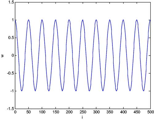For the small value of λ, the graph in Figure 1 is not very close to $\text{cos}\hspace{0.17em}\left(\sqrt{\lambda }x\right).$ However as seen in Figures 2–4, for the larger values of $\lambda ,$ the graph is very close to $\text{cos}\hspace{0.17em}\left(\sqrt{\lambda }x\right).$ For example, for $\lambda =400.001253135326,$ the eigenfunction shown in Figure 4 takes the value 1.00026261584521 at $x=\frac{\pi }{2},$ that is, the obtained eigenfunction is very close to $\text{cos}\hspace{0.17em}\left(\sqrt{400}x\right)=\hspace{0.17em}\text{cos}\hspace{0.17em}\left(20x\right).$ So, as the eigenvalues grow, the corresponding eigenfunctions approach $\text{cos}\hspace{0.17em}\left(\sqrt{\lambda }x\right).$

Figure 1. Graph of the eigenfuntion corresponding to the eigenvalue $\lambda =1.859108072514.$

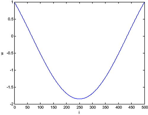
Figure 2. Graph of the eigenfuntion corresponding to the eigenvalue $\lambda =4.371300982731.$

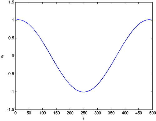
Figure 3. Graph of the eigenfuntion corresponding to the eigenvalue $\lambda =16.033832340360.$

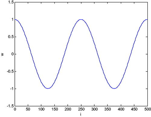
Figure 4. Graph of the eigenfuntion corresponding to the eigenvalue $\lambda =400.001253135326.$

Disclosure statement

The author declares that there is no conflict of interest.

Data availability statement

The data which have been used for the example in Sect. 3 were taken from Dinibutun and Veliev (2013).

References

- Al-Gwaiz, M. A. (2008). Sturm-Liouville theory and its applications. London: Springer.
- Andrew, A. L. (1988). Correction of finite element eigenvalues for problems with natural or periodic boundary conditions. BIT Numerical Mathematics, 28(2), 254–269. doi:https://doi.org/10.1007/BF01934090
- Andrew, A. L. (1989). Correction of finite difference eigenvalues of periodic Sturm-Liouville problems. The Journal of the Australian Mathematical Society. Series B. Applied Mathematics, 30(4), 460–469. doi:https://doi.org/10.1017/S0334270000006391
- Ao, J-j., & Wang, J. (2019). Eigenvalues of Sturm-Liouville problems with distribution potentials on time scales. Quaestiones Mathematicae, 42(9), 1185–1197. doi:https://doi.org/10.2989/16073606.2018.1509394
- Burden, R. L. (2001). Numerical analysis (7th ed.). Pacific Grove, CA: Brooks/Cole.
- Celik, I., & Gokmen, G. (2005). Approximate solution of periodic Sturm-Liouville problems with Chebysev collocation method. Applied Mathematics and Computation, 170(1), 285–295. doi:https://doi.org/10.1016/j.amc.2004.11.038
- Condon, D. J. (1999). Corrected finite difference eigenvalues of periodic Sturm-Liouville problems. Applied Numerical Mathematics, 30(4), 393–401. doi:https://doi.org/10.1016/S0168-9274(98)00093-2
- Dinibutun, S., & Veliev, O. A. (2013). On the estimations of the small periodic eigenvalues. Abstract and Applied Analysis, 2013, 1–11. doi:https://doi.org/10.1155/2013/145967
- Eastham, M. S. P. (1973). The spectral theory of periodic differential equations. Edinburgh: Scottish Academic Press.
- Gao, C., Li, X., & Zhang, F. (2018). Eigenvalues of discrete Sturm-Liouville problems with nonlinear eigenparameter dependent boundary conditions. Quaestiones Mathematicae, 41(6), 773–797. doi:https://doi.org/10.2989/16073606.2017.1401014
- Ghelardoni, P. (1997). Approximations of Sturm-Liouville eigenvalues using boundary value methods. Applied Numerical Mathematics, 23(3), 311–325. doi:https://doi.org/10.1016/S0168-9274(96)00073-6
- Hei, D., & Zheng, M. (2020). Investigation on the dynamic behaviors of a rod fastening rotor based on an analytical solution of the oil film force of the supporting bearing. Journal of Low Frequency Noise, Vibration and Active Control. doi:https://doi.org/10.1177/1461348420912857
- Ji, X. Z. (1994). On a shooting algorithm for Sturm-Liouville eigenvalue problems with periodic and semi-periodic boundary conditions. Journal of Computational Physics, 111(1), 74–80. doi:https://doi.org/10.1006/jcph.1994.1045
- Ji, X., & Wong, Y. S. (1991). Prufer method for periodic and semiperiodic Sturm-Liouville eigenvalue problems. International Journal of Computer Mathematics, 39, 109–123.
- Kutsenko, A. A., Shuvalov, A. L., Poncelet, O., & Norris, A.N. (2013). Spectral properties of a 2D scalar wave equation with 1D periodic coefficients: Application to shear horizontal elastic waves. Mathematics and Mechanics of Solids, 18(7), 677–700. doi:https://doi.org/10.1177/1081286512444750
- Liu, C. S. (2008). A Lie-group shooting method for computing eigenvalues and eigenfunctions of Sturm-Liouville problems. Computer Modeling in Engineering and Sciences, 26(3), 157–168.
- Malathi, V., Suleiman, M. B., & Taib, B. B. (1998). Computing eigenvalues of periodic Sturm–Liouville problems using shooting technique and direct integration method. International Journal of Computer Mathematics, 68(1–2), 119–132. doi:https://doi.org/10.1080/00207169808804682
- Mukhtarov, O., & Yucel, M. (2020). A study of the eigenfunctions of the Singular Sturm–Liouville problem using the analytical method and the decomposition technique. Mathematics, 8(3), 415. doi:https://doi.org/10.3390/math8030415
- Pryce, J. D. (1993). Numerical solution of Sturm-Liouville problems. Oxford: Oxford University Press.
- Vanden Berghe, G., Van Daele, M., & De Meyer, H. (1995). A modified difference scheme for periodic and semiperiodic Sturm–Liouville problems. Applied Numerical Mathematics, 18(1–3), 69–78. doi:https://doi.org/10.1016/0168-9274(95)00067-5
- Wang, H., Zhao, L., & Hu, M. (2017). Eigenvalues of Sturm-Liouville problems with discontinuous boundary conditions. International Journal of Differential Equations, 2017(127), 1–27. doi:https://doi.org/10.1155/2017/2495686
- Yuan, Y., Sun, J., & Zettl, A. (2017). Eigenvalues of periodic Sturm Liouville problems. Linear Algebra and Its Applications, 517, 148–166. doi:https://doi.org/10.1016/j.laa.2016.11.035
- Yucel, U. (2015). Numerical approximations of Sturm–Liouville eigenvalues using Chebyshev polynomial expansions method. Cogent Mathematics, 2(1).