
 ?Mathematical formulae have been encoded as MathML and are displayed in this HTML version using MathJax in order to improve their display. Uncheck the box to turn MathJax off. This feature requires Javascript. Click on a formula to zoom.
Abstract
The time fractional (2, 2, 2) Zakharov-Kuznetsov (ZK) equation and the space-time fractional Zakharov-Kuznetsov-Benjamin-Bona-Mahony (ZKBBM) equation demonstrate the characteristic of shallow water waves, turbulent motion, waves of electro-hydro-dynamics in the local electric field, sound wave, waves of driving flow of fluid, ion acoustic waves in plasmas, traffic flow, financial mathematics, etc. The time-fractional (2, 2, 2) ZK equation is the particular case of the general time-fractional ZK equation, where
represent the space coordinate and
represents the temporal coordinate. Hereinto to evade the complexity and to ascertain soliton solutions of this model, we accept
and in this case, the general ZK equation is called the time-fractional (2, 2, 2) ZK equation. In this article by making use of the concept of fractional complex transformation, the auxiliary equation method is put in use to search the closed form soliton solutions to the above indicated fractional nonlinear equations (FNLEs).The ascertained solutions are in the form of exponential, rational, hyperbolic and trigonometry functions with significant precision. We illustrate the soliton solutions relating to physical concern by setting the definite values of the free parameters through depicting diagram and interpreted the physical phenomena. The developed solutions assert that the method is effective, able to measure NLEEs, influential, powerful and offer vast amount of travelling wave solutions of nonlinear evolution equations in the area of mathematical sciences and engineering.
1. Introduction
Nowadays the fractional nonlinear differential equations (FNLDEs) are broadly used as a significant mathematical tool to depict complex physical phenomena. First, in 1819, Lacroix introduced a definition of fractional derivative based on the usual expression for the -th derivative of the power of a function. After the idea of Lacroix’s definition of fractional derivative, in the history of fractional calculus, within years the fractional calculus and fractional differential equation became a very attractive subject to the mathematicians. Therefore, fractional nonlinear evolution equations (NLEEs) unravel the intricate phenomena. Thus, the study of fractional NLEEs is crucial and much concentration and popularity has gained among the researchers. To recognize further about the fractional NLEE, the definitions, namely the derivative of modified Riemann-Liouville (Jumarie, Citation2006), the derivative of conformable (Khalil, Horani, Yousef, & Sababheh, Citation2014), the derivative Caputo (Caputo & Fabrizio, Citation2015), etc. are familiar in the modern age. NLEEs come forward in various engineering and scientific areas, videlicet quantum mechanics, fluid mechanics, water wave mechanics, chemical kinematics, the modelling of earthquake, biology, optical fibres, electricity, plasma physic, etc. And the exact soliton solutions to nonlinear equation take part in an elementary and crucial role in physical sciences, mathematical physics, engineering, applied sciences.
As a result, the exact solitary wave solutions of fractional NLEEs are very important in order to understand the internal structure of complex physical processes, and many researchers have recently concentrated on finding the closed-form wave solutions of FNLEEs in various fields. Therefore a variety of powerful and modern approaches using computer algebra such as Mathematica or Maple, have recently been developed by several researchers. The available methods are: the auxiliary equation method (Akbar, Ali, & Tanjim, Citation2019; Akbulut, Kaplan, & Bekir, Citation2016; Ismail, Citation2016), the -expansion method (Alam, Akbar, & Mohyud-Din, Citation2014; Bekir & Guner, Citation2013; Islam & Akbar, Citation2018a, Citation2018b, Citation2018c) , the tanh-function method (Ali, Citation2007), the first integral method (Younis, Citation2013), the fractional sub-equation method (Alzaidy, Citation2013), the exp-function method (Zheng, Citation2013; Yokus, Durur, & Ahmad, Citation2020; Yokus, Durur, Ahmad, & Yao, 2020), the modified Kudryashov method (Ege & Misirli, Citation2014), the variational iteration method (He & Latifizadeh, 2020; Neamaty, Agheli, & Darzi, Citation2015), the homotopy perturbation method (Ain et al., Citation2020; Anjum & Ain, Citation2020; Fereidoon, Yaghoobi, & Davoudabadi, Citation2011; He, Citation2019a, Citation2019b; Yu, He, & Garcia, 2019), the modified simple equation method (Islam & Akbar, Citation2018c), the Jacobi elliptic method (Zheng & Feng, Citation2014), the differential transformation method (Rabtah, Erturk, & Momani, Citation2010), the modified trial equation method (Bulut, Baskonus, & Pandir, Citation2013), the finite element method (Deng, Citation2009), the Adomin decomposition method (Dahmani, Mesmoudi, & Bebbouchi, Citation2008), the Taylor series method (He et al., Citation2020), the variational iteration algorithm-I (Ahmad & Khan, 2019; Ahmed, Khan, & Cesarano, Citation2019) the variational iteration algorithm-II (Ahmad, Seadawy, & Khan, 2020; Ahmad, Seadawy, Khan, & Thounthong, 2020), the Riccati transformation method (Bazighifan, Ahmad, & Yao, Citation2020), the meshless techniques (Inc et al., Citation2020), the improve Bernoulli sub-equation function method (Islam & Akbar, 2020), etc.
The wave solutions to fractional NLEEs are noteworthy to analyze real world problems and recently many researchers contemplated to examine the exact wave solutions of fractional NLEEs in different areas. In the literature, the time fractional (2, 2, 2) Zakharov-Kuznetsov(ZK) equation and the space-time Zakharov-Kuznetsov-Benjamin-Bona-Mahony (ZKBBM) equation are investigated through the He’s homotopy perturbation method (Yildirim & Gulkanat, Citation2010), the modified Kudryashov method (Munro & Parkes, Citation1999), the first integral method (Hossein, Refahi, & Hadi, Citation2015), the tanh-coth method (Hossam & Ghany, Citation2013), the fractional sub-equation method (Ray & Sahoo, Citation2015), the -expansion method (Ali, Iqbal, & Mohyud-Din, Citation2016a), the exp-function method (Ali, Iqbal, & Mohyud-Din, Citation2016b), the
-expansion method(Shakeel & Mohyud-Din, Citation2015), and the variational iteration method (Molliq, Noorani, Hashim, & Ahmad, Citation2009; Torvattanabun & Koonprasert, Citation2017), the
-expansion method (Roshid et al., Citation2014) etc.
To our foremost interpretation the (2, 2, 2) ZK equation and the ZKBBM equation were not examined through the auxiliary equation approach. Therefore, the key objective of this article is to examine the wide-ranging, advanced, compatible and the further general closed form travelling wave solutions to the ZKBBM and the (2, 2, 2) ZK equations by means of the auxiliary equation method and exhibit the physical implication for its definite values of the established solutions. The method is a recently formulated effectual and thriving method to look into advanced and broad-ranging soliton solutions to NLEEs. We also provide graphs of solutions to interpret inner physical mechanisms.
This article is sorted as follows: In section 2, physical meaning of fractional derivative is discussed. In Section 3, we have briefly illustrated the auxiliary equation method. In Section 4, we figured out the solutions. In Section 5, the results are portrayed and discussed. Finally, we provide conclusion in Section 6.
2. Fractional derivative and its explanation
This part covers fractional calculus and fractional derivative (Atangana, Citation2017; Baleanu, Golmankhaneh, Golmankhaneh, & Nigmatullin, Citation2010; Brouers, Citation2014; Brouers & Sotolongo-Costa, Citation2006; Chen & Liang, Citation2017; Fan et al., Citation2015; Golmankhaneh & Baleanu, Citation2016; Gomez-Aguilar, Razo-Hernandez, & Granados-Lieberman, Citation2014; He, 2014, Citation2018; He, Elagan, & Li, Citation2012; Hu & He, Citation2016; Liu & He, Citation2018; Pan, Zheng, Liu, Liu, & Chen, 2018) in order to understand the physical meaning of fractional derivative and demonstrate its geometrical interpretation.
Fractional calculus (FC) is a useful technique for understanding the evolution of memory systems, which are typically dissipative and complicated (Chen & Liang, Citation2017; Gomez-Aguilar et al., Citation2014). This is the key benefit of FC in judgement with the classical integer-order models in which such effects are in fact ignored. In time-domain investigations, the physical meaning of fractional derivatives is useful. This is because fractional differential equations (FDEs) with well-known derivatives behave similarly to ordinary differential equations (ODEs) with a broad scientific understanding. Many physical phenomena can be explained using the fractional-order derivative and therefore it is very important for the FC to provide details (Baleanu et al., Citation2010; Gomez-Aguilar et al., Citation2014). FC models physical systems more accurately than traditional systems in a variety of applications. The fractals theory is another big field that necessitates the use of FC (Gomez-Aguilar et al., Citation2014; He, Citation2014). The development of the fractals theory has opened more perspective for the theory of fractional derivatives, particularly in describing dynamical processes in self-similar and permeable configurations. Fractional-order derivatives are defined in different ways. The Riemann-Liouville fractional derivative, the Jumarie's modified Riemann-Liouville fractional derivative (Jumarie, Citation2006), the conformal fractional derivative (Khalil et al., Citation2014), the Beta-derivative (Atangan, Baleanu, & Alsaedi, Citation2016), the Caputo derivative (Caputo & Fabrizio, Citation2015), etc. are realistic and extensively used. The fractional complex transform was first proposed by Li and He (Citation2010) to transmute a FDE into an ODE. This fractional complex transformation plays a significant role in understanding the physical meaning of the fractional derivative.
Understanding the physical meaning of fractional derivative is important in order to achieve better outcomes in the realistic behalf. The fractional-order model is more functional than the integer-order model, and nonlinear FDE research has piqued the interest of academics in various fields of science, engineering, and mathematical physics.
Fractal geometry, fractal calculus and fractional calculus have been becoming burning topics in both engineering and mathematical physics for non-differential solutions (He, Citation2018; He et al., Citation2012; Hu & He, Citation2016). Fractal theory is the theoretical basis for the fractal space-time (He, Citation2014) and fractional calculus was introduced in Newton’s time, and it has developed into a very important matter where classic mechanics becomes ineffectual to illustrate any phenomena on the porous size scale (He, Citation2018; Hu & He, Citation2016; Pan et al., Citation2018).
Two-scale mathematics is required to disclose the lost information owing to the lower-dimensional method. In general, one scale is identified by usage where standard calculus is used, while a second scale is used to expose lost information where the continuum hypothesis is not allowed and fractal calculus is used (He, Citation2014). The fractional calculus can simply be transferred into its classical partner via the two-scale transform, making two-scale thermodynamics very promising. The FDE can be translated into traditional differential equations using the two-scale transform, which are easy to solve. The fractal calculus is moderately new; it can efficiently deal with kinetics, which is always identified the fractal kinetics (Brouers, Citation2014; Brouers & Sotolongo-Costa, Citation2006; Chen & Liang, Citation2017; He, Citation2018), where the fractal time substituting the continuous time. It is declared that time does be discontinuous in microphysics where fractal kinetics gets place on extremely small time scale.
The fractal derivative (Hausdorff derivative) on time fractal is defined in the following (Atangana, Citation2017; Golmankhaneh & Baleanu, Citation2016; He, Citation2018; Liu & He, Citation2018):
(2.1)
(2.1)
where
is the fractal dimension of time.
A further general definition is presented below
(2.2)
(2.2)
where
is the fractal dimension of space.
The fractional gradient is of the form (He, Citation2018):
(2.3)
(2.3)
For the three-dimension case, the fractal gradient can be shown in the form
(2.4)
(2.4)
where
is the partial fractal derivative identified by
(2.5)
(2.5)
where
is the fractional dimensions in the
-direction,
is the lowest hierarchical distance.
The fractal derivative present in EquationEquation (2.5)(2.5)
(2.5) has widely been utilized to deal with hierarchical formations (Fan et al., Citation2015) with large success. A fractal space is always not isotropic, i.e. the fractal dimensions in
-directions are different. By replacing the EquationEquation (2.5)
(2.5)
(2.5) by the following one
(2.6)
(2.6)
where
are respectively, the fractal dimensions in
-directions
(2.7)
(2.7)
(2.8)
(2.8)
(2.9)
(2.9)
where
are the minimal porous sized in
-directions, respectively.
To establish laws in fractal media, it is essential to set up the idea of fractal velocity, which is presented below (in the ) (He, Citation2018):
(2.10)
(2.10)
EquationEquation (2.10)(2.10)
(2.10) can be recognized as an average velocity of a particle moving from A to B in the fractal space (where AB is the discontinuous line in the ) (He, Citation2018). The conservation of mass involves
(2.11)
(2.11)
Figure 1. Fractal gradient.
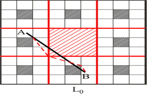
Figure 2. A control volume in a fractal medium.
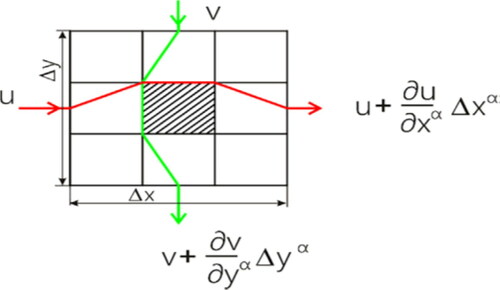
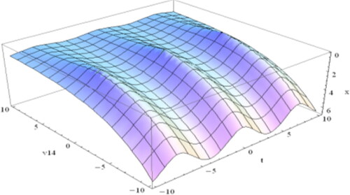
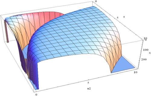
Figure 1. Plot of the spike shape soliton of Equation(4.1.9)(4.1.9)
(4.1.9) when
and
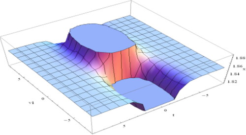
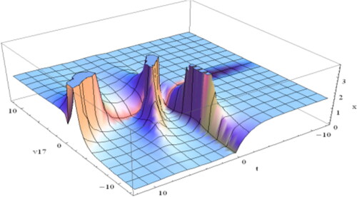
Figure 2. Plot of Equation(4.1.17)(4.1.17)
(4.1.17) for
and
which is singular periodic soliton.
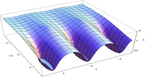
Figure 3. Design of the periodic soliton of Equation(4.1.23)(4.1.23)
(4.1.23) for
and
The results mass equation in a fractal media in the following:
(2.12)
(2.12)
In general case, the mass equation can be shown as follows:
(2.13)
(2.13)
where
is the density of the fluid and
are the respectively, the fractional dimensions in the in
-directions and
are the respectively, the fractal velocity in
-directions.
The fractal streamlines in a fractal media, it yields:
(2.14)
(2.14)
where
are, the respectively, the fractal velocity in
-directions, are defined as,
Introducing the new space and then defined by
and
i.e. the space
can be approximately measured as a smooth one, making the solution much simple and straightforward. We infer that as the order of the fractional derivative increases, the settling time reduces, as does the sensitivity of the settling time to the order of the derivative. As the order of the derivative drops, the rise time increases, becoming more sensitive as the time delay reduces.
3. Methodology
Consider the general fractional NLEE is of the form:
(3.1)
(3.1)
where
is wave function,
is a polynomial in
and its partial derivatives. In order to determine the solution of EquationEquation (3.1)
(3.1)
(3.1) by means of the auxiliary equation method, we have to present the ensuing steps:
Step 1: Let us consider the travelling wave variable (He et al., Citation2012; Li & He, Citation2010)
(3.2)
(3.2)
for real fractional differential equations and
are fractional order derivatives and
and they may equal or not.
The above wave transformations translate the EquationEquation (3.1)(3.1)
(3.1) into the following ODE:
(3.3)
(3.3)
where
is a polynomial in
and its derivatives, wherein
Step 2: We integrate EquationEquation (3.3)(3.3)
(3.3) term by term one or more times according to possibility in this step.
Step 3: In accordance with auxiliary equation method we reveal the travelling wave solution of EquationEquation (3.3)(3.3)
(3.3) as:
(3.4)
(3.4)
where
and
are constants to be examined, such that
and
satisfies the subsequent supportive equation:
(3.5)
(3.5)
wherein the prime stands for derivative with respect to
and
are parameters.
Step 4: The positive integer presents in Equation(3.4)
(3.4)
(3.4) can be calculated by balancing the nonlinear and linear terms of the highest order occurring in Equation(3.3)
(3.3)
(3.3) .
Step 5: Assembling Equation(3.4)(3.4)
(3.4) together Equation(3.5)
(3.5)
(3.5) into Equation(3.3)
(3.3)
(3.3) and the value of
obtained in Step 4, we get a polynomial of
Collecting all the terms of the similar power
where
and setting them to zero yields a system of algebraic equations with the constants
and
can be established and solving them yields the values of the unknown parameters. As the general solution of Equation(3.5)
(3.5)
(3.5) is known, inserting the values of
and
into (3.4), we accomplish broad-spectrum and new exact solitary wave solutions to the EquationEquation (3.3)
(3.3)
(3.3) .
Step 6: For different values of
and
and their relationship, Equation(3.5)
(3.5)
(3.5) provides different types of general solutions.
4. Extraction of solutions
In this section, we construct compatible, convenient and further general soliton solutions to the fractional (2, 2, 2) ZK equation and the ZKBBM equation by means of the introduced method. Furthermore, we discuss about the graphical representations and physical significance of the attained solutions.
4.1. Analysis of the (2, 2, 2) time-fractional ZK equation
In this sub-section, we determine some new soliton solutions to the (2, 2, 2) time-fractional ZK equation by putting use of the auxiliary equation method. The (2, 2, 2) time-fractional ZK equation (Yildirim & Gulkanat, Citation2010) is:
(4.1.1)
(4.1.1)
The fractional wave transformation Equation(3.2)(3.2)
(3.2) reshapes the EquationEquation (4.1.1)
(4.1.1)
(4.1.1) into the following nonlinear equation:
(4.1.2)
(4.1.2)
EquationEquation (4.1.2)(4.1.2)
(4.1.2) implies by integrating
(4.1.3)
(4.1.3)
where
is an integrating constant.
Balancing between the highest order linear and nonlinear terms appearing in EquationEquation (4.1.3)(4.1.3)
(4.1.3) , we obtain
Therefore, we employ the transformation
Then EquationEquation (4.1.3)
(4.1.3)
(4.1.3) turns into the following nonlinear ODE:
(4.1.4)
(4.1.4)
where
is an integrating constant.
Now, balancing the two highest orders nonlinear terms happening in (Equation4.1.4(4.1.4)
(4.1.4) ) yields
Therefore, it is clear that the shape of the solution of EquationEquation (4.1
(4.1.1)
(4.1.1) .4) is
(4.1.5)
(4.1.5)
Inserting (Equation4.1.5(4.1.5)
(4.1.5) ), Equation(3.5)
(3.5)
(3.5) into (Equation4.1.4
(4.1.4)
(4.1.4) ) and collecting the coefficients the powers of
and setting them zero, we reach a set of algebraic equations (for minimalism which are not gathered here) for
and
Solving the system of algebraic equations by means of the computer algebra software, such as, Mathematica, offer the solutions as:
(4.1.6)
(4.1.6)
where
and
are free parameters and
is an integrating constant.
We establish the subsequent soliton solutions based on the data assembled in (Equation4.1.6(4.1.6)
(4.1.6) ) and using the solutions of Equation(3.5)
(3.5)
(3.5) :
When and
substituting the values of the constants assembled in (Equation4.1.6
(4.1.6)
(4.1.6) ) into (Equation4.1.5
(4.1.5)
(4.1.5) ) and simplifying, we attain the following travelling wave solutions
(4.1.7)
(4.1.7)
or
(4.1.8)
(4.1.8)
By means of the transformation the solution (Equation4.1.7
(4.1.7)
(4.1.7) ) and (Equation4.1.8
(4.1.8)
(4.1.8) ) become
(4.1.9)
(4.1.9)
or
(4.1.10)
(4.1.10)
For and
putting the values arranged in (Equation4.1.6
(4.1.6)
(4.1.6) ) into (Equation4.1.5
(4.1.5)
(4.1.5) ) and with the transformation
we achieve
(4.1.11)
(4.1.11)
or
(4.1.12)
(4.1.12)
When
and
then
making use of (Equation4.1.6
(4.1.6)
(4.1.6) ), (Equation4.1.5
(4.1.5)
(4.1.5) ) and the transformation
the travelling wave solutions turns into
(4.1.13)
(4.1.13)
or
(4.1.14)
(4.1.14)
When
and
then
Employing (Equation4.1.6
(4.1.6)
(4.1.6) ), (Equation4.1.5
(4.1.5)
(4.1.5) ) and the value
we gain
(4.1.15)
(4.1.15)
or
(4.1.16)
(4.1.16)
In the case of and
and
Now applying (Equation4.1.6
(4.1.6)
(4.1.6) ) and (Equation4.1.5
(4.1.5)
(4.1.5) ) and
the solutions provide
(4.1.17)
(4.1.17)
or
(4.1.18)
(4.1.18)
For
and
Putting in use (Equation4.1.6
(4.1.6)
(4.1.6) ) into (Equation4.1.5
(4.1.5)
(4.1.5) ) and with the aid of the result
we accomplish
(4.1.19)
(4.1.19)
or
(4.1.20)
(4.1.20)
For then
and inserting (Equation4.1.6
(4.1.6)
(4.1.6) ) into (Equation4.1.5
(4.1.5)
(4.1.5) ) and using
the solution becomes the form
(4.1.21)
(4.1.21)
When
and
then
Now using (Equation4.1.6
(4.1.6)
(4.1.6) ) and (Equation4.1.5
(4.1.5)
(4.1.5) ) and the result
we derive
(4.1.22)
(4.1.22)
or
(4.1.23)
(4.1.23)
For and
it if found
and
By means of (Equation4.1.6
(4.1.6)
(4.1.6) ), (Equation4.1.5
(4.1.5)
(4.1.5) ) and the result
we examine
(4.1.24)
(4.1.24)
While then
and
Substituting the values from (Equation4.1.6
(4.1.6)
(4.1.6) ) into (Equation4.1.5
(4.1.5)
(4.1.5) ) and considering the result
we determine
(4.1.25)
(4.1.25)
When and
then
Now applying (Equation4.1.6
(4.1.6)
(4.1.6) ), (Equation4.1.5
(4.1.5)
(4.1.5) ) and
the wave solution becomes
(4.1.26)
(4.1.26)
For and
then
By the aid of (Equation4.1.6
(4.1.6)
(4.1.6) ), (Equation4.1.5
(4.1.5)
(4.1.5) ) and the result
we establish
(4.1.27)
(4.1.27)
Applying the condition we can get
Now setting the constants arranged in (Equation4.1.6
(4.1.6)
(4.1.6) ) into (Equation4.1.5
(4.1.5)
(4.1.5) ) and also setting
we attain
(4.1.28)
(4.1.28)
For we ascertain
and
Applying (Equation4.1.6
(4.1.6)
(4.1.6) ) and (Equation4.1.5
(4.1.5)
(4.1.5) ) and
we achieve
(4.1.29)
(4.1.29)
When then
Making use (Equation4.1.6
(4.1.6)
(4.1.6) ) and (Equation4.1.5
(4.1.5)
(4.1.5) ) and the result
the soliton solution provides
(4.1.30)
(4.1.30)
Making use the condition we get
Now for
and putting the values in (Equation4.1.6
(4.1.6)
(4.1.6) ) into (Equation4.1.5
(4.1.5)
(4.1.5) ), we ascertain
(4.1.31)
(4.1.31)
For
Now taking (Equation4.1.6
(4.1.6)
(4.1.6) ), (Equation4.1.5
(4.1.5)
(4.1.5) ) and using
the solution becomes in the form
(4.1.32)
(4.1.32)
While then
Now considering (Equation4.1.6
(4.1.6)
(4.1.6) ) and (Equation4.1.5
(4.1.5)
(4.1.5) ) and the result
we obtain
(4.1.33)
(4.1.33)
For the conditions and
then
Making use of (Equation4.1.6
(4.1.6)
(4.1.6) ) and (Equation4.1.5
(4.1.5)
(4.1.5) ) and the result
the travelling wave solution is given below
(4.1.34)
(4.1.34)
When then
Substituting the values scheduled in (Equation4.1.6
(4.1.6)
(4.1.6) ) into (Equation4.1.5
(4.1.5)
(4.1.5) ) and applying the result
we gain
(4.1.35)
(4.1.35)
Here, for all above solutions, and
are arbitrary constant.
The erstwhile accomplished solutions are compatible, reliable and capable to interpret the demandable model in the ion-acoustic waves in plasma, the sound waves, the electromagnetic field, the optical fibres, the material science, the signal processing wave, the financial mathematics, the traffic flow, etc.
4.2. Solutions to the space-time fractional ZKBBM equation
Let us consider the nonlinear ZKBBM equation given below (Hossein et al., 2015):
(4.2.1)
(4.2.1)
where
and
are physical parameters.
Making use of the travelling wave variable (3.2), EquationEquation (4.2(4.1.1)
(4.1.1) .1) converts to the ODE and integrating once, yields
(4.2.2)
(4.2.2)
where
stands for an integral constant.
We balance the highest order derivative for linear term and the highest order nonlinear term
taking place in (Equation4.2.2
(4.2.2)
(4.2.2) ), gives
Therefore, the solution outline of EquationEquation (4.2
(4.1.1)
(4.1.1) .2) is:
(4.2.3)
(4.2.3)
Since
are unknown, they must be determined.
Inserting the solution (Equation4.2.3(4.2.3)
(4.2.3) ) together with Equation(3.5)
(3.5)
(3.5) into (Equation4.2.2
(4.2.2)
(4.2.2) ) and setting the coefficients of
of its different power to zero, a set of simultaneous algebraic equations are attained (for simplicity these algebraic equations are not present here) for
and
Solving the equations by the aid of symbolic computation software Maple, we extract the solution of unknowns as
(4.2.4)
(4.2.4)
where
We evaluate the following soliton solutions using the values gathered in (Equation4.2.4(4.2.4)
(4.2.4) ) and the solutions of (3.5).
When but
inserting the values assembled in (Equation4.2.4
(4.2.4)
(4.2.4) ) into (Equation4.2.3
(4.2.3)
(4.2.3) ) and simplifying, we attain the soliton solutions
(4.2.5)
(4.2.5)
or
(4.2.6)
(4.2.6)
When and
using (Equation4.2.3
(4.2.3)
(4.2.3) ) and (Equation4.2.4
(4.2.4)
(4.2.4) ), the solutions turns into
(4.2.7)
(4.2.7)
or
(4.2.8)
(4.2.8)
If
and
then
Making use of (Equation4.2.4
(4.2.4)
(4.2.4) ) and (Equation4.2.3
(4.2.3)
(4.2.3) ), we secure
(4.2.9)
(4.2.9)
or
(4.2.10)
(4.2.10)
When
and
then
Now, embedding the values accumulated in (Equation4.2.4
(4.2.4)
(4.2.4) ) into (Equation4.2.3
(4.2.3)
(4.2.3) ), we ascertain
(4.2.11)
(4.2.11)
or
(4.2.12)
(4.2.12)
While and
then
Thus, from (Equation4.2.4
(4.2.4)
(4.2.4) ) and (Equation4.2.3
(4.2.3)
(4.2.3) ), we accomplish
(4.2.13)
(4.2.13)
or
(4.2.14)
(4.2.14)
For the relation and
it is found
Inserting (Equation4.2.4
(4.2.4)
(4.2.4) ) into (Equation4.2.3
(4.2.3)
(4.2.3) ), we attain the soliton solutions as
(4.2.15)
(4.2.15)
or
(4.2.16)
(4.2.16)
While then
and applying (Equation4.2.3
(4.2.3)
(4.2.3) ) and (Equation4.2.4
(4.2.4)
(4.2.4) ), we find out
(4.2.17)
(4.2.17)
When
and
then
Setting the result scheduled in (Equation4.2.4
(4.2.4)
(4.2.4) ) into (Equation4.2.3
(4.2.3)
(4.2.3) ), the soliton turns out to be
(4.2.18)
(4.2.18)
or
(4.2.19)
(4.2.19)
For
and
it is obtained
and substituting the values amassed in (Equation4.2.4
(4.2.4)
(4.2.4) ) into (Equation4.2.3
(4.2.3)
(4.2.3) ), we determine
(4.2.20)
(4.2.20)
For and
then
Now using (Equation4.2.4
(4.2.4)
(4.2.4) ) and (Equation4.2.3
(4.2.3)
(4.2.3) ), we achieve
(4.2.21)
(4.2.21)
By applying the condition we attain
and with the aid of the values scheduled in (Equation4.2.4
(4.2.4)
(4.2.4) ) into (Equation4.2.3
(4.2.3)
(4.2.3) ), we carry out
(4.2.22)
(4.2.22)
For it becomes
Now inserting the values managed in (Equation4.2.4
(4.2.4)
(4.2.4) ) into (Equation4.2.3
(4.2.3)
(4.2.3) ), we attain
(4.2.23)
(4.2.23)
If then
Putting the values into (Equation4.2.3
(4.2.3)
(4.2.3) ) from (Equation4.2.4
(4.2.4)
(4.2.4) ), the soliton solution becomes
(4.2.24)
(4.2.24)
The soliton solution turns into the following form, for and by means of (Equation4.2.4
(4.2.4)
(4.2.4) ) into (Equation4.2.3
(4.2.3)
(4.2.3) )
(4.2.25)
(4.2.25)
For then
Now exploiting (Equation4.2.4
(4.2.4)
(4.2.4) ) and (Equation4.2.3
(4.2.3)
(4.2.3) ), the wave solution becomes
(4.2.26)
(4.2.26)
For the case and
then
and using (Equation4.2.4
(4.2.4)
(4.2.4) ) and (Equation4.2.3
(4.2.3)
(4.2.3) ), we found
(4.2.27)
(4.2.27)
Here, for all above solutions, and
are arbitrary constants.
Inserting the values produces a trivial solution, which is not mentioned here because it has no physical implication. Furthermore, when
and
are used to input the values from (Equation4.2.4
(4.2.4)
(4.2.4) ) into (Equation4.2.3
(4.2.3)
(4.2.3) ), trivial solutions are found, which are not depicted here. For
with
on the other hand, the wave solution takes the form of a trivial solution, which is not given here.
It is decisive to note that the above-achieved solutions of the ZKBBM equation are further generic and advanced, and some of them are accessible in the literature, as well as several primal solutions are originated that were not revealed in the previous study. The upstretched solutions can be used to investigate signal processing in optical fibres, gravitational waves, water wave mechanics, turbulent motion, and fluid driving flow, etc.
5. Graphical representation and discussion
5.1. Graphical representation of the solutions
We will demonstrate the profile of the graphs and describe the physical features of the resulting solutions to the space-time fractional ZKBBM equations and the (2, 2, 2) time fractional ZK equation in this paragraph.
In addition, for more details, we have illustrated a variety of figures (–) of the solution (Equation4.1.25(4.1.25)
(4.1.25) ) in the interval
of the ZK equation and for the solution (Equation4.2.6
(4.2.6)
(4.2.6) ) in the interval
of the ZKBBM equation for the values of all involved parameters are fixed but the fractal parameter
varies. Consequently, the effect of the fractional order is shown in the following figures. For different fractional orders, the profiles of the solution (Equation4.1.25
(4.1.25)
(4.1.25) ) of the ZK equation are:
As can be seen from the portrayals above, the fractional order has a substantial impact on the profile of solitary waves. When
the shape shown in of the solution (Equation4.1.25
(4.1.25)
(4.1.25) ) of the ZK equation is a multiple singular kink soliton. And the profiles are marked in for the values
respectively, and it is seen that the profiles change with the change of the fractional order
The wave profile presented for the solution (Equation4.2.6(4.2.6)
(4.2.6) ) of the ZKBBM equation, the influence of fractional
order is shown in the underneath:
We observe that the shape is a singular periodic soliton when The profiles are identified in for the values
respectively. Therefore, we can conclude that the fractal order P has a significant impact on wave profiles.
Figure 15. For
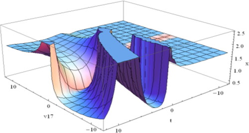
Figure 16. For
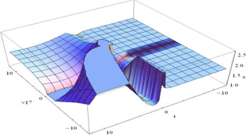
Figure 17. For
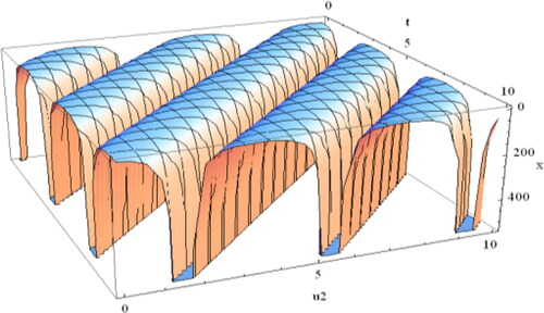
Figure 18. For
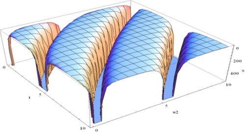
Figure 19. For
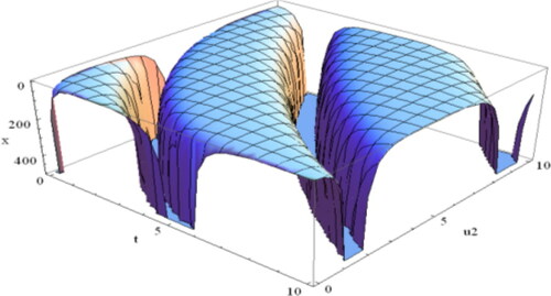
Figure 20. For
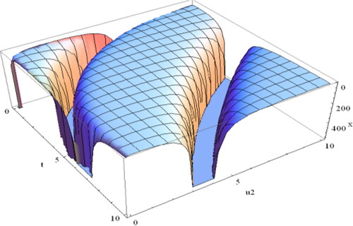
Figure 21. For
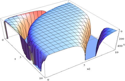
Figure 22. For
5.2. Physical significance of the solutions
In this earlier section, we portrayed some 3 D representations using symbolic computing software Mathematica to figure out the studied solutions for both equations. For minimalism, we have depicted some graphs from the obtained adequate solutions, videlicet the solutions (Equation4.1.9(4.1.9)
(4.1.9) ), (Equation4.1.17
(4.1.17)
(4.1.17) ), (Equation4.1.23
(4.1.23)
(4.1.23) ), (Equation4.1.31
(4.1.31)
(4.1.31) ) and (Equation4.1.34
(4.1.34)
(4.1.34) ) of the ZK equation. The remaining obtained solutions of this equation are sketched in the same way which are similar of the above illustrated figures. Therefore, these graphs are not shown here for the sake of simplicity.
Also for simplicity, we have sketched a few graphs of the ZKBBM equation, namely for the solutions (Equation4.2.6(4.2.6)
(4.2.6) ), (Equation4.2.11
(4.2.11)
(4.2.11) ), (Equation4.2.12
(4.2.12)
(4.2.12) ), Equation(
(4.2.14)
(4.2.14) Equation4.2.14
(4.2.14)
(4.2.14) Equation)
(4.2.14)
(4.2.14) and Equation(
(4.2.24)
(4.2.24) Equation4.2.24
(4.2.24)
(4.2.24) Equation)
(4.2.24)
(4.2.24) . We also make out that the other figures of the remaining solutions which are alike to above outlined figures. Therefore, for simplicity these figures are not been displayed here.
We also observe that, the sketched graphs are different nature of well-known shapes of wave solutions inasmuch as, kink shape wave solution, singular kink shape solutions, spike shape wave solutions and singular periodic solutions, etc.
Figure 4. Design the spike shape soliton of Equation(4.1.31)(4.1.31)
(4.1.31) while
and
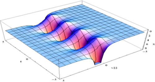
Figure 5. Sketch of the soliton of Equation(4.1.34)(4.1.34)
(4.1.34) when
and
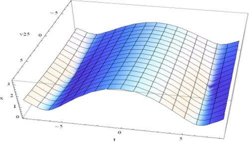
Figure 6. Sketch of the singular periodic soliton Equation(4.2.6)(4.2.6)
(4.2.6) for
and

Figure 7. Plot of Equation(4.2.11)(4.2.11)
(4.2.11) which is spike shape soliton for
and
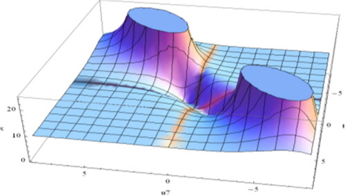
Figure 8. Plot the singular kink of Equation(4.2.12)(4.2.12)
(4.2.12) for
and
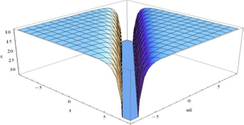
Figure 9. Profile of Equation(4.2.14)(4.2.14)
(4.2.14) is the singular periodic soliton for
and
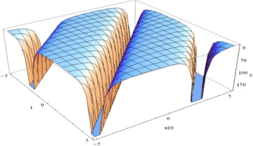
Figure 10. Profile of Equation(4.2.24)(4.2.24)
(4.2.24) is the kink shape soliton for
and
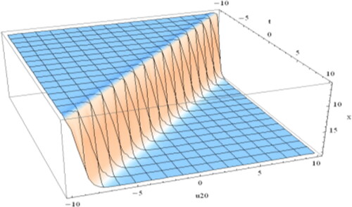
Figure 11. For
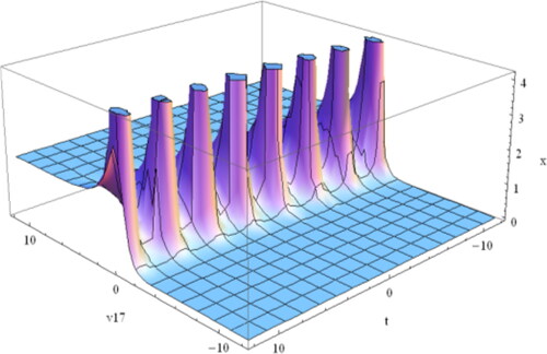
Figure 12. For
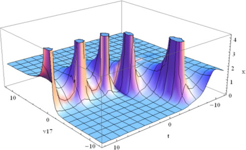
Figure 13. For
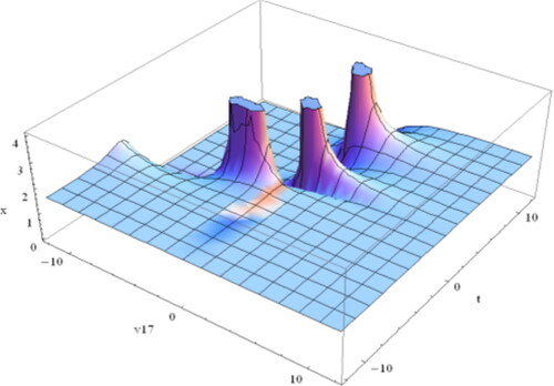
Figure 14. For
6. Conclusion
In this article, we have established wide-ranging, useful and further developed closed-form soliton solutions to the space-time fractional ZKBBM equation and the time fractional (2, 2, 2) ZK equation. The closed-form wave solutions are established in terms of trigonometric, exponential, hyperbolic, and rational functions, as well as their integration with a number of free parameters and the fractal dimension Theoretically, the fractional dimension
has a role in the nature of waves. To demonstrate this, we have sketched the solution (Equation4.1.25
(4.1.25)
(4.1.25) ) and (Equation4.2.6
(4.2.6)
(4.2.6) ) for different values of
keeping all the other parameters constant. The figures confirm that as the value of
changes, so does the nature of the wave, establishing the effect of
The attained solutions might play vital role in ion acoustic waves, electro-hydro-dynamical waves in the local electric field, shallow water waves, turbulent motion, driving flow of fluid, heat transfer, etc. The results obtained demonstrate that the auxiliary equation method is further developed, effective algorithm, powerful and can be employed to unravel further fractional nonlinear equations in physical science and engineering.
Acknowledgement
The authors are grateful to the anonymous referees for their insightful remarks and ideas on how to enhance the article.
Disclosure statement
No potential conflict of interest was reported by the authors.
References
- Ahmad, H., & Khan, T. A. (2019). Variational iteration algorithm-I with an auxiliary parameter for wave-like vibration equations. Journal of Low Frequency Noise, Vibration and Active Control, 38(3–4), 1113–1132. doi:https://doi.org/10.1177/1461348418823126
- Ahmed, H., Khan, T. A., & Cesarano, C. (2019). Numerical solutions of coupled Burgers’ equations. Axioms, 8(4), 119.
- Ahmad, H., Seadawy, A. R., & Khan, T. A. (2020). Study on numerical solution of dispersive water wave phenomena by using a reliable modification of variational iteration algorithm. Mathematics and Computers in Simulation, 177, 13–23. doi:https://doi.org/10.1016/j.matcom.2020.04.005
- Ahmad, H., Seadawy, A. R., Khan, T. A., & Thounthong, P. (2020). Analytic approximate solutions for some nonlinear parabolic dynamical wave equations. Journal of Taibah University for Science, 14(1), 346–358. doi:https://doi.org/10.1080/16583655.2020.1741943
- Ain, Q. T., He, J. H., Anjum, N., & Ali, M. (2020). The fractional complex transform: A novel approach to the time-fractional Schrodinger equation. Fractals, 28(07), 2050141–2055578. doi:https://doi.org/10.1142/S0218348X20501418
- Akbar, M. A., Ali, N. H. M., & Tanjim, T. (2019). Outset of multiple soliton solutions to the nonlinear Schrodinger equation and the coupled Burgers equation. Journal of Physics Communications, 3(9), 095013. doi:https://doi.org/10.1088/2399-6528/ab3615
- Akbulut, A., Kaplan, M., & Bekir, A. (2016). Auxiliary equation method for fractional differential equations with modified Riemann-Liouville derivative. International Journal of Nonlinear Science and Numerical Simulation, 174, 13–20.
- Alam, M. N., Akbar, M. A., & Mohyud-Din, S. T. (2014). A novel (G′/G)-expansion method and its application to the Boussinesq equations. Chinese Physics B, 23(2), 020203. doi:https://doi.org/10.1088/1674-1056/23/2/020203
- Ali, A., Iqbal, A., & Mohyud-Din, S. T. (2016a). Traveling wave solutions of generalized Zakharov-Kuznetsov-Benjamin-Bona-Mahony and simplified modified form of Camassa-Holm equation method by using exp (−ϕ(η))-expansion method. Egyptian Journal of Basic and Applied Sciences, 3(2), 134–140. doi:https://doi.org/10.1016/j.ejbas.2016.01.001
- Ali, A., Iqbal, M. A., & Mohyud-Din, S. T. (2016b). Solitary wave solutions Zakharov-Kuznetsov-Benjamin-Bona-Mahony (ZKBBM) equation. Journal of the Egyptian Mathematical Society, 24(1), 44–48. doi:https://doi.org/10.1016/j.joems.2014.10.008
- Ali, A. H. A. (2007). The modified extended tanh-function method for solving coupled mKdV and coupled Hirota-Satsuma coupled KdV equations. Physics Letters A, 363(5–6), 420–425. doi:https://doi.org/10.1016/j.physleta.2006.11.076
- Alzaidy, J. F. (2013). The fractional sub-equation method and exact analytical solutions for some nonlinear fractional PDEs. British Journal of Mathematics & Computer Science, 3(2), 153–163. doi:https://doi.org/10.9734/BJMCS/2013/2908
- Anjum, N., & Ain, Q.T. (2020). Application of He’s fractional derivative and fractional complex transform for time fractional Camassa-Holm equation. Thermal Science, 24(5 Part A), 3023–3030. doi:https://doi.org/10.2298/TSCI190930450A
- Atangan, A., Baleanu, D., & Alsaedi, A. (2016). Analysis of time-fractional Hunter-Saxton equation: A model of neumatic liquid crystal. Open Physics, 14(1), 145–149. doi:https://doi.org/10.1515/phys-2016-0010
- Atangana, A. (2017). Fractal-fractional differentiation and integration: Connecting fractal calculus and fractional calculus to predict complex system. Chaos, Solitons & Fractals, 102, 396–406. doi:https://doi.org/10.1016/j.chaos.2017.04.027
- Baleanu, D., Golmankhaneh, A. K., Golmankhaneh, A. K., & Nigmatullin, R. R. (2010). Newtonian law with memory. Nonlinear Dynamics, 60(1–2), 81–86. doi:https://doi.org/10.1007/s11071-009-9581-1
- Bazighifan, O., Ahmad, H., & Yao, S.-W. (2020). New oscillation criteria for advanced differential equations of fourth order. Mathematics, 8(5), 728. doi:https://doi.org/10.3390/math8050728
- Bekir, A., & Guner, O. (2013). Exact solutions of nonlinear fractional differential equation by (G′/G)-expansion method. Chinese Physics B, 22(11), 110202–110206. doi:https://doi.org/10.1088/1674-1056/22/11/110202
- Brouers, F. (2014). The fractal (BSf) kinetics equation and its approximations. Journal of Modern Physics, 05(16), 1594–1601. doi:https://doi.org/10.4236/jmp.2014.516160
- Brouers, F., & Al-Musawi, T. J. (2018). Brouers-Sotolongo fractal kinetics versus fractional derivative kinetics: A new strategy to analyze the pollutants sorption kinetics in porous materials. Journal of Hazardous Materials, 350, 162–168. doi:https://doi.org/10.1016/j.jhazmat.2018.02.015
- Brouers, F., & Sotolongo-Costa, O. (2006). Generalized fractal kinetics in complex systems (application to biophysics and biotechnology). Physica A: Statistical Mechanics and Its Applications, 368(1), 165–175. doi:https://doi.org/10.1016/j.physa.2005.12.062
- Bulut, H., Baskonus, H. M., & Pandir, Y. (2013). The modified trial equation method for fractional wave equation and time fractional generalized Burgers equation. Abstract and Applied Analysis, 2013, 1–8. doi:https://doi.org/10.1155/2013/636802
- Caputo, M., & Fabrizio, M. A. (2015). A new definition of fractional derivatives without singular kernel. Progress in Fractional Differentiation and Applications, 1, 73–85.
- Chen, W., & Liang, Y. (2017). New methodologies in fractional and fractal derivatives modeling. Chaos, Solitons & Fractals, 102, 72–77. doi:https://doi.org/10.1016/j.chaos.2017.03.066
- Dahmani, Z., Mesmoudi, M. M., & Bebbouchi, R. (2008). The foam-drainage equation with time and space fractional derivative solved by the ADM method. Journal of Qualitative Theory of Differential Equations, 30, 1–10.
- Deng, W. (2009). Finite element method for the space and time fractional Fokker-Planck equation. SIAM Journal on Numerical Analysis, 47(1), 204–226. doi:https://doi.org/10.1137/080714130
- Ege, S. M., & Misirli, E. (2014). Solutions of space-time fractional foam drainage equation and the fractional Klein-Gordon equation by use of modified Kudryashov method. International Journal of Research in Advent Technology, 2(3), 384–388.
- Fan, J., Wang, L.-L., Liu, F.-J., Liu, Z., Liu, Y., & Zhang, S. (2015). Model of moisture diffusion in fractal media. Thermal Science, 19(4), 1161–1166. doi:https://doi.org/10.2298/TSCI1504161F
- Fereidoon, A., Yaghoobi, H., & Davoudabadi, M. (2011). Application of the homotopy perturbation method for solving the foam drainage equation. International Journal of Differential Equations, 2011, 1–13. doi:https://doi.org/10.1155/2011/864023
- Golmankhaneh, A. K., & Baleanu, D. (2016). New derivatives on the fractal subset of real-line. Entropy, 8(2), 1–13.
- Gomez-Aguilar, J. F., Razo-Hernandez, R., & Granados-Lieberman, D. (2014). A physical interpretation of fractional calculus in observables terms: Analysis of the fractional time constant and the transitory response. Revista Mexicana De Fisica, 60, 32–38.
- He, C. H., Shen, Y., Ji, F. Y., & He, J. H. (2020). Taylor series solution for fractal Bratu-type equation arising in electro spinning process. Fractals, 28(01), 2050011. doi:https://doi.org/10.1142/S0218348X20500115
- He, J. H. (2014). A tutorial review on fractal space-time and fractional calculus. International Journal of Theoretical Physics, 53(11), 3698–3718. doi:https://doi.org/10.1007/s10773-014-2123-8
- He, J. H. (2018). Fractal calculus and its geometrical explanation. Results in Physics, 10, 272–276. doi:https://doi.org/10.1016/j.rinp.2018.06.011
- He, J. H. (2019a). The simpler, the better: Analytical methods for nonlinear oscillators and fractional oscillators. Journal of Low Frequency Noise, Vibration and Active Control, 38(3–4), 1252–1260. doi:https://doi.org/10.1177/1461348419844145
- He, J. H. (2019b). The simplest approach to nonlinear oscillators. Results in Physics, 15(2019), 102546. doi:https://doi.org/10.1016/j.rinp.2019.102546
- He, J. H. (2020). Taylor series solution for a third order boundary value problem arising in architectural engineering. Ain Shams Engineering Journal, 11(4), 1411–1414. doi:https://doi.org/10.1016/j.asej.2020.01.016
- He, J. H., Elagan, S. K., & Li, Z. B. (2012). Geometrical explanation of the fractional complex transform and derivative chain rule for fractional calculus. Physics Letters A, 376(4), 257–259. doi:https://doi.org/10.1016/j.physleta.2011.11.030
- He, J. H., & Latifizadeh, H. (2020). A general numerical algorithm for nonlinear differential equations by the variational iteration method. International Journal of Numerical Methods for Heat & Fluid Flow, 30(11), 4797–4810. doi:https://doi.org/10.1108/HFF-01-2020-0029
- Hossam, A. & Ghany, (2013). Exact solutions for stochastic fractional Zakharov-Kuznetsov equations. Chinese Journal of Physics, 51(5), 875–881.
- Hossein, A., Refahi, S. A., & Hadi, R. (2015). Exact solutions for the fractional differential equations by using the first integral method. Nonlinear Engineering, 4(1), 15–22.
- Hu, Y., & He, J. H. (2016). On fractal space-time and fractional calculus. Thermal Science, 20(3), 773–777. doi:https://doi.org/10.2298/TSCI1603773H
- Inc, M., Khan, M. N., Ahmad, I., Yao, S.-W., Ahmad, H., & Thounthong, P. (2020). Analysing time-fractional exotic options via efficient local meshless method. Results in Physics, 19, 103385. doi:https://doi.org/10.1016/j.rinp.2020.103385
- Islam, M. N., & Akbar, M. A. (2018a). New exact wave solutions to the space-time fractional coupled Burger equations and the space-time fractional foam drainage equation. Cogent Physics, 5(1), 1422957–1422918. doi:https://doi.org/10.1080/23311940.2017.1422957
- Islam, M. N., & Akbar, M. A. (2018b). Closed form solutions to the coupled space-time fractional evolution equations in mathematical physics through analytical method. Journal of Mechanics of Continua and Mathematical Sciences, 13(2), 1–23. doi:https://doi.org/10.26782/jmcms.2018.06.00001
- Islam, M. N., & Akbar, M. A. (2018c). Closed form exact solutions to the higher dimensional fractional Schrodinger equation via the modified simple equation method. Journal of Applied Mathematics and Physics, 06(01), 90–102. doi:https://doi.org/10.4236/jamp.2018.61009
- Islam, M. E., & Akbar, M. A. (2020). Stable wave solutions to the Landau-Ginzburg-Higgs equation and the modified equal width wave equation using the IBSEF method. Arab Journal of Basic and Applied Sciences, 27(1), 270–278. doi:https://doi.org/10.1080/25765299.2020.1791466
- Ismail, A. (2016). Exact solution for fractional DDEs via auxiliary equation method coupled with the fractional complex transform. Mathematical Method of Applied Science, 39(18), 5619–5625.
- Jumarie, G. (2006). Modified Riemann-Liouville derivative and fractional Taylor series of non-differentiable functions further results. Computers & Mathematics with Applications, 51(9–10), 1367–1376. doi:https://doi.org/10.1016/j.camwa.2006.02.001
- Khalil, R. R., Horani, M. A. H. H., Yousef, A., & Sababheh, M. (2014). A new definition of fractional derivative. Journal of Computational and Applied Mathematics, 264, 65–70. doi:https://doi.org/10.1016/j.cam.2014.01.002
- Li, Z. B., & He, J. H. (2010). Fractional complex transform for fractional differential equations. Mathematical and Computational Applications, 15(5), 970–973. doi:https://doi.org/10.3390/mca15050970
- Liu, P., & He, J. H. (2018). Geometrical potential: An explanation on of nano-fibers wettability. Thermal Science, 22(1 Part A), 33–38. doi:https://doi.org/10.2298/TSCI160706146L
- Molliq, R. Y., Noorani, M. S. M., Hashim, I., & Ahmad, R. R. (2009). Approximate solutions of fractional Zakharov-Kuznetsov equations by VIM. Journal of Computational and Applied Mathematics, 233(2), 103–108. doi:https://doi.org/10.1016/j.cam.2009.03.010
- Munro, S., & Parkes, E. J. (1999). The derivation of a modified Zakharov-Kuznetsov equations and the stability of its solutions. Journal of Plasma Physics, 62(3), 305–317. doi:https://doi.org/10.1017/S0022377899007874
- Neamaty, A., Agheli, B., & Darzi, R. (2015). Variational iteration method and He’s polynomials for time fractional partial differential equations. Progress in Fractional Differentiation and Applications, 1(1), 47–55.
- Pan, M., Zheng, L., Liu, F., Liu, C., & Chen, X. (2018). A spatial-fractional thermal transport model for nanofluid in porous media. Applied Mathematical Modelling, 53, 622–634. doi:https://doi.org/10.1016/j.apm.2017.08.026
- Rabtah, A. A., Erturk, R. S., & Momani, S. (2010). Solution of fractional oscillator by using differential transformation method. Computers & Mathematics with Applications, 59(3), 1356–1362. doi:https://doi.org/10.1016/j.camwa.2009.06.036
- Ray, S. S., & Sahoo, S. (2015). New exact solutions of fractional Zakharov-Kuznetsov and modified Zakharov-Kuznetsov equations using fractional sub-equation method. Communications in Theoretical Physics, 63(1), 25–30. doi:https://doi.org/10.1088/0253-6102/63/1/05
- Roshid, H. O., Alam, M. N., Hossain, M. M., Ullah, M. S., Islam, R., & Akbar, M. A. (2014). Exact traveling wave solutions for the (2 + 1)-dimensional ZK-BBM equation by exp (−ϕ(η))-expansion method. Global Journal of Science and Frontier Research, 14(2), 1–5.
- Shakeel, M., & Mohyud-Din, S. T. (2015). New (G′/G)-expansion method and its application to the ZK-BBM equation. Journal of the Association of Arab University for Basic and Applied Sciences, 18, 66–81.
- Torvattanabun, M., & Koonprasert, S. (2017). Exact travelling wave solutions to the ZKBBM nonlinear evolution equation using the VIM combined with the improved generalized tanh-coth method. Applied Mathematical Sciences, 11(64), 3141–3152. doi:https://doi.org/10.12988/ams.2017.711337
- Yokus, A., Durur, H., & Ahmad, H. (2020). Hyperbolic type solutions for the couple Boiti-Leon-Pempinellisystem. Facta Universitatis, Series: Mathematics and Informatics, 35(2), 523–531. doi:https://doi.org/10.22190/FUMI2002523Y
- Yokus, A., Durur, H., Ahmad, H., & Yao, S.-W. (2020). Construction of different types analytic solutions for the Zhiber-Shabat equation. Mathematics, 8(6), 908. doi:https://doi.org/10.3390/math8060908
- Younis, M. (2013). The first integral method for time-space fractional differential equations. Journal of Advanced Physics, 2(3), 220–223. doi:https://doi.org/10.1166/jap.2013.1074
- Yildirim, A., & Gulkanat, Y. (2010). Analytical approach to fractional Zakharov-Kuznetsov equations by He’s homotopy perturbation method. Communication and Theatrical Physics, 53(6), 1005–1010.
- Yu, D.N., He, J.H., & Garcia, A.G. (2019). Homotopy perturbation method with an auxiliary parameter for nonlinear oscillators. Journal of Low Frequency Noise, Vibration and Active Control, 38(3–4), 1540–1554. doi:https://doi.org/10.1177/1461348418811028
- Zheng, B. (2013). Exp-function method for solving fractional partial differential equations. TheScientificWorldJournal, 2013, 465723. doi:https://doi.org/10.1155/2013/465723
- Zheng, B & Feng, Q. (2014). The Jacobi elliptic equation method for solving fractional partial differential equations. Abstract and Applied Analysis, 2014, 1–9. doi:https://doi.org/10.1155/2014/249071