On an approximate solution of a boundary value problem for a nonlinear integro-differential equation

Abstract

The aim of this work is to discuss the solvability of a boundary value problem for a nonlinear integro-differential equation. First, we derive an equivalent nonlinear Fredholm integral equation (NFIE) to this problem. Second, we prove the existence of a solution to the NFIE using the Krasnosel’skii fixed point theorem under verifying some sufficient conditions. Third, we solve the NFIE numerically and study the convergence rate via methods based upon applying the modified Adomian decomposition method and Liao’s homotopy analysis method. As applications, some examples are illustrated to support our work. The results in this work refer to both methods are efficient and converge rapidly, but the homotopy analysis method may converge faster when we succeed in choosing the optimal homotopy control parameter.

Keywords:

• Boundary value problem
• integro-differential equations
• existence
• uniqueness
• modified Adomian’s decomposition method
• homotopy analysis method

2020 MATHEMATICS SUBJECT CLASSIFICATION:

• 45Gxx
• 34A12
• 45L05
• 45G10

1. Introduction

Many problems arising in applied physics, biology, chemistry and engineering can be described using mathematical models that depend on utilizing integral and differential operators with imposed conditions. For example, the so-called Chandrasekhar H-function that appears in the radiative transfer processes, is defined in terms of integral equation. The evolution of biological populations is characterized by employing delayed integro-differential equations of the Volterra type. Continuous medium-nuclear reactors are analysed using models that employ systems of integro-differential equations. Also, there are the singular integral equations that occur during the process of formulating mixed boundary value problems in mathematical physics, especially in solid mechanics and elasticity. Using the Green function approach, we can transform many partial differential equations to equivalent integral equations. So, trying to find solutions for these equations attracts many researchers. Because we cannot determine the exact solutions for most of these equations, “many numerical” or “semi-analytic” techniques are developed to overcome this gap. From these methods, there are the Adomian decomposition method (ADM), homotopy perturbation method (HPM), variational iteration method (VIM), homotopy analysis method (HAM) and many other methods, see Abdou, Soliman, and Abdel-Aty (2020), Hamoud and Ghadle (2018), He (2020a, 2020b), Mirzaee and Alipour (2019), Rezabeyk, Abbasbandy, and Shivanian (2020), Saeedi, Tari, and Babolian (2020) among others. These techniques can be applied to find approximate solutions for a large class of linear and nonlinear integral equations and many functional equations as well. Also, in some special cases, when the series solution converges to a known function we can get a closed form-solution using these methods. For example, Wazwaz (2010) confirmed that the VIM is very reliable in solving first- and second-kind integral equations of the Volterra type and most calculations can be significantly reduced. Alhendi, Shammakh, and Al-Badrani (2017) found that the VIM and HPM are very effective when applying them to solve quadratic fractional integro-differential equations. Elborai, Abdou, and Youssef (2013) studied the mean square convergence of the series solution for a stochastic integro-differential equation and estimated the truncation error by the ADM. Kurt and Tasbozan (2019) utilized the HAM to solve the modified Burgers equation. Singh, Kumar, Baleanu, and Rathore (2018) used the Sumudu transform along with the HAM to find approximate solutions to some fractional equations of the Drinfeld–Sokolov–Wilson type. Hetmaniok, Słota, Trawiński, and Wituła (2014) explained the applicability of the HAM in solving nonlinear integral equations of second kind. Hamoud, Ghadle, and Atshan (2019) applied the MADM (modified Adomian’s decomposition method) to find an approximate solution for a class of fractional nonlinear integro-differential equation of the Caputo-Volterra–Fredholm type. Issa, Hamoud, and Ghadle (2021) used the MADM, VIM and HPM to solve a fuzzy integro-differential equation of the Volterra type numerically and compared the results, see Adomian (1994), Alidema and Georgieva (2018), Bakodah, Al-Mazmumy, and Almuhalbedi (2019), Liao (2012), Maitama and Zhao (2019) and Singh, Nelakanti, and Kumar (2014) for more applications regarding these elegant methods and the references therein.

The current article discusses the solvability of a two-point boundary value problem for a nonlinear integro-differential equation in the form (1.1) $$\begin{array}{c}\mu \frac{d^2\psi (x)}{d{x}^2}+A_1(x)\frac{d\psi (x)}{dx}+A_2(x)\psi (x)\hfill \\ -\lambda {\int }_a^{b}K(x-y){[\psi (y)]}^{p}dy=f(x),\hspace{1em}a\le x\le b.\hfill \end{array}$$(1.1) subject to the boundary conditions (1.2) $$\psi (a)={\zeta }_0,\hspace{1em}\psi (b)={\zeta }_1,\hspace{1em}\{{\zeta }_0,{\zeta }_1\}\in \mathbb{R}.$$(1.2) where $p\ge 0$ is a finite non-negative integer. The parameters $\{\mu ,\lambda \}$ are two non zero real parameters. The functions $A_1,A_2,f$ and the kernel K are known functions satisfying certain conditions to be assigned in the next section while $x\mapsto \psi (x)$ is the sought function to be determined in the space $C^2([a,b],\mathbb{R}),$ (see Def. (2.1)). The present form of Eq. (1.1)(1.1) $$\begin{array}{c}\mu \frac{d^2\psi (x)}{d{x}^2}+A_1(x)\frac{d\psi (x)}{dx}+A_2(x)\psi (x)\hfill \\ -\lambda {\int }_a^{b}K(x-y){[\psi (y)]}^{p}dy=f(x),\hspace{1em}a\le x\le b.\hfill \end{array}$$(1.1) is not discussed before to the best of our knowledge. This work is organized as follows. In the section “Outcomes for existence and uniqueness”, we derive a corresponding nonlinear Fredholm integral equation (NFIE) for Equation (1.1)(1.1) $$\begin{array}{c}\mu \frac{d^2\psi (x)}{d{x}^2}+A_1(x)\frac{d\psi (x)}{dx}+A_2(x)\psi (x)\hfill \\ -\lambda {\int }_a^{b}K(x-y){[\psi (y)]}^{p}dy=f(x),\hspace{1em}a\le x\le b.\hfill \end{array}$$(1.1) under verifying condition (1.2). Then, we apply the Krasnosel’skii fixed point theorem to prove the existence of solutions for this NFIE under satisfying some sufficient conditions. The uniqueness of this solution is investigated as well. The convergence of solution and truncation error is studied in the “Analysis of MADM” section. The homotopy analysis technique is applied to problem (1.1) under verifying condition (1.2) in the “Analysis of HAM” section. Next, we present some applications in the section “Numerical and analytical outcomes”. The section “Conclusion” is devoted to the discussion of results.

2. Outcomes for existence and uniqueness

In order to prove Thm. (2.1) we suppose the following postulates.

1. the functions A₁ and A₂ are elements in the space $C([a,b],\mathbb{R}).$

2. the known free function f belongs to the space $C^2([a,b];\mathbb{R}).$

3. the known kernel $(x,y)\mapsto K(x-y)$ is continuous in $x\forall y\in [a,b]$ with values in $\mathbb{R}$ and: $${\left({\int }_a^b{\left(K(x-y)\right)}^{2}dy\right)}^{\frac{1}{2}}\le \gamma ,\hspace{1em}\forall x\in [a,b],\gamma >0.$$

Theorem 2.1.

Let conditions $(i)-(\mathit{iii})$ are satisfied. Then the boundary value problem (1.1)-(1.2) is equivalent to the following NFIE. (2.1) $$\begin{array}{c}\mu u(x)+{\int }_a^b\left(H(x,t)-\lambda {\int }_a^{b}S(x,y;1)M_2(y,t)dy\right)u(t)dt\hfill \\ =F(x)+\lambda {\int }_a^b\sum _{l=2}^{p}S(x,y;l){\left[{\int }_a^b{M}_2(y,t)u(t)dt\right]}^{l}dy.\hfill \end{array}$$(2.1) where: (2.2) $$u(x):={\psi }^{″}(x),$$(2.2) (2.3) $$H(x,t):=\frac{1}{(b-a)}\{\begin{array}{cc}{H}_1(x,t)=(t-a)\left(A_1(x)-(b-x)A_2(x)\right),\hfill & \text{if}\hspace{1em}a\le t\le x,\hfill \\ H_2(x,t)=(t-b)\left(A_1(x)-(a-x)A_2(x)\right),\hfill & \text{if}\hspace{1em}x<t\le b.\hfill \end{array}$$(2.3) (2.4) $$S(x,y;l):=\left(\begin{array}{c}p\\ l\end{array}\right)\frac{K(x-y)}{{(b-a)}^p}{\left[{\zeta }_0(b-y)+{\zeta }_1(y-a)\right]}^{p-l},$$(2.4) (2.5) $$M_2(y,t):=\{\begin{array}{cc}(b-y)(a-t),\hfill & \text{if}\hspace{1em}a\le t\le y,\hfill \\ (a-y)(b-t),\hfill & \text{if}\hspace{1em}y\le t\le b.\hfill \end{array}$$(2.5) (2.6) $$\omega (x):=\frac{1}{(b-a)}({\zeta }_0[-A_1(x)+(b-x)A_2(x)]+{\zeta }_1[A_1(x)+(x-a)A_2(x)]),$$(2.6) (2.7) $$F(x):=f(x)-\omega (x)+\lambda {\int }_a^{b}S(x,y;0)dy.$$(2.7)

Proof.

Let ${\psi }^{″}(x)=u(x),$ where the function $x\mapsto u(x)$ is an element in the space $C([a,b];\mathbb{R}).$ So, we have (2.8) $${\psi }^{\prime }(x)={\psi }^{\prime }(a)+{\int }_a^{x}u(t)dt.$$(2.8) and (2.9) $$\psi (x)={\zeta }_0+(x-a){\psi }^{\prime }(a)+{\int }_a^x(x-t)u(t)dt.$$(2.9)

Putting x = b in Equation (2.9)(2.9) $$\psi (x)={\zeta }_0+(x-a){\psi }^{\prime }(a)+{\int }_a^x(x-t)u(t)dt.$$(2.9) , then using the result in Equations (2.8)(2.8) $${\psi }^{\prime }(x)={\psi }^{\prime }(a)+{\int }_a^{x}u(t)dt.$$(2.8) and (2.9)(2.9) $$\psi (x)={\zeta }_0+(x-a){\psi }^{\prime }(a)+{\int }_a^x(x-t)u(t)dt.$$(2.9) gives (2.10) $${\psi }^{\prime }(x)=\frac{1}{(b-a)}\left[({\zeta }_1-{\zeta }_0)+{\int }_a^b{M}_1(x,t)u(t)dt\right].$$(2.10) (2.11) $$\psi (x)=\frac{1}{(b-a)}\left[{\zeta }_0(b-x)+{\zeta }_1(x-a)+{\int }_a^b{M}_2(x,t)u(t)dt\right].$$(2.11) where: $$M_1(x,t)=\{\begin{array}{cc}(t-a),\hfill & \text{if}\hspace{1em}a\le t\le x,\hfill \\ (t-b),\hfill & \text{if}\hspace{1em}x<t\le b.\hfill \end{array}$$ $$M_2(x,t)=\{\begin{array}{cc}(b-x)(a-t),\hfill & \text{if}\hspace{1em}a\le t\le x,\hfill \\ (a-x)(b-t),\hfill & \text{if}\hspace{1em}x\le t\le b.\hfill \end{array}$$

It is easy to see that (2.12) $${\left[\psi (x)\right]}^p=\frac{1}{{(b-a)}^p}\sum _{l=0}^p\left(\begin{array}{c}p\\ l\end{array}\right){\left[{\zeta }_0(b-x)+{\zeta }_1(x-a)\right]}^{p-l}{\left({\int }_a^b{M}_2(x,t)u(t)dt\right)}^l.$$(2.12)

Substituting Equations (2.10) (2.11)(2.11) $$\psi (x)=\frac{1}{(b-a)}\left[{\zeta }_0(b-x)+{\zeta }_1(x-a)+{\int }_a^b{M}_2(x,t)u(t)dt\right].$$(2.11) and (2.12)(2.12) $${\left[\psi (x)\right]}^p=\frac{1}{{(b-a)}^p}\sum _{l=0}^p\left(\begin{array}{c}p\\ l\end{array}\right){\left[{\zeta }_0(b-x)+{\zeta }_1(x-a)\right]}^{p-l}{\left({\int }_a^b{M}_2(x,t)u(t)dt\right)}^l.$$(2.12) in Equation (1.1)(1.1) $$\begin{array}{c}\mu \frac{d^2\psi (x)}{d{x}^2}+A_1(x)\frac{d\psi (x)}{dx}+A_2(x)\psi (x)\hfill \\ -\lambda {\int }_a^{b}K(x-y){[\psi (y)]}^{p}dy=f(x),\hspace{1em}a\le x\le b.\hfill \end{array}$$(1.1) gives (2.13) $$\begin{array}{c}\mu u(x)+\frac{1}{(b-a)}{\int }_a^b[A_1(x)M_1(x,t)+A_2(x)M_2(x,t)]u(t)dt\\ -\frac{\lambda }{{(b-a)}^p}\underset{a}{\overset{b}{\int }}\sum _{l=0}^p\left(\begin{array}{c}p\\ l\end{array}\right)K(x-y){[{\zeta }_0(b-y)+{\zeta }_1(y-a)]}^{p-l}{\left(\underset{a}{\overset{b}{\int }}{M}_2(y,t)u(t)dt\right)}^{l}dy\\ =f(x)-\frac{1}{(b-a)}({\zeta }_0[-A_1(x)+(b-x)A_2(x)]+{\zeta }_1[A_1(x)+(x-a)A_2(x)]).\end{array}$$(2.13)

It is easy to figure out $[A_1(x)M_1(x,t)+A_2(x)M_2(x,t)]=(b-a)H(x,t).$ Set $$\begin{array}{c}S(x,y;l)=\left(\begin{array}{c}p\\ l\end{array}\right)\frac{K(x-y)}{{(b-a)}^p}{\left[{\zeta }_0(b-y)+{\zeta }_1(y-a)\right]}^{p-l}.\\ \omega (x)=\frac{1}{(b-a)}({\zeta }_0[-A_1(x)+(b-x)A_2(x)]+{\zeta }_1[A_1(x)+(x-a)A_2(x)]).\end{array}$$

Therefore, we have $$\mu u(x)+{\int }_a^{b}H(x,t)u(t)dt-\lambda {\int }_a^b\sum _{l=0}^{p}S(x,y;l){\left[{\int }_a^b{M}_2(y,t)u(t)dt\right]}^{l}dy=f(x)-\omega (x).$$ Using Equation (2.7)(2.7) $$F(x):=f(x)-\omega (x)+\lambda {\int }_a^{b}S(x,y;0)dy.$$(2.7) yields $$\begin{array}{cc}\mu u(x)\hfill & +{\int }_a^b\left(H(x,t)-\lambda {\int }_a^{b}S(x,y;1)M_2(y,t)dy\right)u(t)dt\hfill \\ \hfill & =F(x)+\lambda {\int }_a^b\sum _{l=2}^{p}S(x,y;l){\left[{\int }_a^b{M}_2(y,t)u(t)dt\right]}^{l}dy.\hfill \end{array}$$ The converse can be done easily and thereby it is omitted. The proof is completed. □

Remark 2.1.

It is worth mentioning that Thm. (2.1) is valid whether the kernel $K(x-y)$ is continuous or has a singularity of the weak type at the straight line y = x.

Definition 2.1.

By a solution for the boundary value problem Equation (1.1)(1.1) $$\begin{array}{c}\mu \frac{d^2\psi (x)}{d{x}^2}+A_1(x)\frac{d\psi (x)}{dx}+A_2(x)\psi (x)\hfill \\ -\lambda {\int }_a^{b}K(x-y){[\psi (y)]}^{p}dy=f(x),\hspace{1em}a\le x\le b.\hfill \end{array}$$(1.1) , we mean proving the existence of a function $\psi \in C^2([a,b];\mathbb{R})$ satisfying Equation (1.1)(1.1) $$\begin{array}{c}\mu \frac{d^2\psi (x)}{d{x}^2}+A_1(x)\frac{d\psi (x)}{dx}+A_2(x)\psi (x)\hfill \\ -\lambda {\int }_a^{b}K(x-y){[\psi (y)]}^{p}dy=f(x),\hspace{1em}a\le x\le b.\hfill \end{array}$$(1.1) , and the boundary conditions (1.2).

Let the constant $l\in \{a\in \mathbb{Z}:0\le a\le p\}.$ We define the following positive real constants. $$\begin{array}{cc}{d}^{*}(l)\hfill & =\left({\zeta }_1^{2p-2l}+{\zeta }_1^{2p-2l-1}{\zeta }_0+{\zeta }_1^{2p-2l-2}{\zeta }_0^2+\cdots +{\zeta }_0^{2p-2l}\right).\hfill \\ c^{*}(l)\hfill & =\left(\begin{array}{c}p\\ l\end{array}\right)\frac{\gamma {(b-a)}^{2l+\frac{1}{2}}{\left(d^{*}(l)\right)}^{\frac{1}{2}}}{{(2p-2l+1)}^{\frac{1}{2}}}.\hfill \end{array}$$

We consider the following assumption.

• (iv) $(\beta +\left|\lambda \right|c^{*}(1))<\left|\mu \right|,\text{where}\beta :=(b-a)(\left|\right|A_1|{|}_{\infty }+(b-a)|\left|A_2\right|{|}_{\infty }).$

Theorem 2.2.

Let conditions $(i)-(iv)$ are verified. Then the NFIE (2.1) possesses continuous solutions.

Proof.

Let ${\Omega }_r=\left\{u\in C([a,b],\mathbb{R}):\left|\right|u|{|}_{\infty }=\underset{x\in [a,b]}{\sup }|u(x)|\le r\right\}.$ The radius r is a finite positive solution for the equation $\left|\lambda \right|{\sum }_{l=2}^p{c}^{*}(l)r^l+(\beta +\left|\lambda \right|c^{*}(1)-\left|\mu \right|)r+\left|\right|F|{|}_{\infty }=0.$ Let u₁, u₂ be any two functions in the set Ω_r. Define the following two operators. (2.14) $$\begin{array}{cc}(T{u}_1)(x)\hfill & =\frac{1}{\mu }F(x)-\frac{1}{\mu }{\int }_a^b\left(H(x,t)-\lambda {\int }_a^{b}S(x,y;1)M_2(y,t)dy\right)u_1(t)dt.\hfill \\ (W{u}_2)(x)\hfill & =\frac{\lambda }{\mu }{\int }_a^b\sum _{l=2}^{p}S(x,y;l){\left[{\int }_a^b{M}_2(y,t)u_2(t)dt\right]}^{l}dy.\hfill \end{array}$$(2.14)

Applying the Cauchy inequality and then, simplifying the right-hand side yield $$\begin{array}{cc}\left|(T{u}_1)(x)\right|\hfill & \le \frac{1}{\left|\mu \right|}|F(x)|+\frac{r}{\left|\mu \right|}{\int }_a^b\left|H(x,t)\right|dt+\frac{\left|\lambda \right|r}{\left|\mu \right|}{\int }_a^b{\int }_a^b\left|S(x,y,1)\right|\left|M_2(x,t)\right|d\mathit{ydt}\hfill \\ \hfill & \le \frac{1}{\left|\mu \right|}|F(x)|+\frac{\beta r}{\left|\mu \right|}+\frac{\left|\lambda \right|pr}{\left|\mu \right|{(b-a)}^{p-3}}{\int }_a^b\frac{\left|K(x-y)\right|}{|({\zeta }_1-{\zeta }_0)y+({\zeta }_{0}b-{\zeta }_{1}a){|}^{1-p}}dy\hfill \\ \hfill & \le \frac{1}{\left|\mu \right|}|F(x)|+\frac{\beta r}{\left|\mu \right|}+\frac{\left|\lambda \right|p{(b-a)}^{\frac{5}{2}}{(d^{*}(1))}^{\frac{1}{2}}r}{\left|\mu \right|{(2p-1)}^{\frac{1}{2}}}{\left({\int }_a^b{\left(K(x-y)\right)}^{2}dy\right)}^{\frac{1}{2}}.\hfill \end{array}$$

Using condition (iii), passing the supremum over $x\in [a,b]$ and then, utilizing the value of $c^{*}(1)$ give (2.15) $${\Vert T{u}_1\Vert }_{\infty }\le \frac{1}{\left|\mu \right|}\left|\right|F|{|}_{\infty }+\frac{1}{\left|\mu \right|}\left(\beta +\left|\lambda \right|c^{*}(1)\right)r.$$(2.15)

Using similar arguments as we used above implies (2.16) $$\begin{array}{cc}\left|\right|W(u_2)|{|}_{\infty }\hfill & \le \frac{\left|\lambda \right|}{\left|\mu \right|}{\int }_a^b\sum _{l=2}^p|S(x,y;l)|{\left({\int }_a^b\left|M_2(y,t)u_2(t)\right|dt\right)}^{l}dy\hfill \\ \hfill & \le \frac{\left|\lambda \right|}{\left|\mu \right|}\sum _{l=2}^p\left(\begin{array}{c}p\\ l\end{array}\right){(b-a)}^{3l-p}{r}^l\left({\int }_a^b\frac{\left|K(x-y)\right|}{|({\zeta }_1-{\zeta }_0)y+({\zeta }_{0}b-{\zeta }_{1}a){|}^{2l-2p}}dy\right)\hfill \\ \hfill & \le \frac{\left|\lambda \right|}{\left|\mu \right|}\sum _{l=2}^p\left(\begin{array}{c}p\\ l\end{array}\right)\frac{{(b-a)}^{2l+\frac{1}{2}}{(d^{*}(l))}^{\frac{1}{2}}{r}^l}{{(2p-2l+1)}^{\frac{1}{2}}}{\left({\int }_a^b{\left(K(x-y)\right)}^{2}dy\right)}^{\frac{1}{2}}\hfill \\ \hfill & =\frac{\left|\lambda \right|}{\left|\mu \right|}\sum _{l=2}^p{c}^{*}(l)r^l.\hfill \end{array}$$(2.16)

Using Equations (2.15)(2.15) $${\Vert T{u}_1\Vert }_{\infty }\le \frac{1}{\left|\mu \right|}\left|\right|F|{|}_{\infty }+\frac{1}{\left|\mu \right|}\left(\beta +\left|\lambda \right|c^{*}(1)\right)r.$$(2.15) and (2.16)(2.16) $$\begin{array}{cc}\left|\right|W(u_2)|{|}_{\infty }\hfill & \le \frac{\left|\lambda \right|}{\left|\mu \right|}{\int }_a^b\sum _{l=2}^p|S(x,y;l)|{\left({\int }_a^b\left|M_2(y,t)u_2(t)\right|dt\right)}^{l}dy\hfill \\ \hfill & \le \frac{\left|\lambda \right|}{\left|\mu \right|}\sum _{l=2}^p\left(\begin{array}{c}p\\ l\end{array}\right){(b-a)}^{3l-p}{r}^l\left({\int }_a^b\frac{\left|K(x-y)\right|}{|({\zeta }_1-{\zeta }_0)y+({\zeta }_{0}b-{\zeta }_{1}a){|}^{2l-2p}}dy\right)\hfill \\ \hfill & \le \frac{\left|\lambda \right|}{\left|\mu \right|}\sum _{l=2}^p\left(\begin{array}{c}p\\ l\end{array}\right)\frac{{(b-a)}^{2l+\frac{1}{2}}{(d^{*}(l))}^{\frac{1}{2}}{r}^l}{{(2p-2l+1)}^{\frac{1}{2}}}{\left({\int }_a^b{\left(K(x-y)\right)}^{2}dy\right)}^{\frac{1}{2}}\hfill \\ \hfill & =\frac{\left|\lambda \right|}{\left|\mu \right|}\sum _{l=2}^p{c}^{*}(l)r^l.\hfill \end{array}$$(2.16) give (2.17) $$\begin{array}{cc}\left|\right|T(u_1)+W(u_2)|{|}_{\infty }\hfill & \le \left|\right|T(u_1)|{|}_{\infty }+||W(u_2)|{|}_{\infty }\hfill \\ \hfill & \le \frac{1}{\left|\mu \right|}\left|\right|F|{|}_{\infty }+\frac{1}{\left|\mu \right|}\left(\beta +\left|\lambda \right|c^{*}(1)\right)r+\frac{\left|\lambda \right|}{\left|\mu \right|}\sum _{l=2}^p{c}^{*}(l)r^l=r.\hfill \end{array}$$(2.17)

Therefore, $T(u_1)+W(u_2)\in {\Omega }_r,\forall u_1,u_2\in {\Omega }_r.$ Now, suppose $x_1<x_2$ be two elements in $[a,b].$ The functions F, H₁ and H₂ are continuous in x from applying conditions $(i)-(\mathit{iii})$ and therefore, we have (2.18) $$\begin{array}{c}\left|(T{u}_1)(x_2)-(T{u}_1)(x_1)\right|\hfill \\ \le \frac{1}{\left|\mu \right|}\left|F(x_2)-F(x_1)\right|+\frac{r}{\left|\mu \right|(b-a)}{\int }_a^{x_1}\left|H_1(x_2,t)-H_1(x_1,t)\right|dt\hfill \\ +\frac{r}{\left|\mu \right|(b-a)}\left({\int }_{x_2}^b\left|H_2(x_2,t)-H_2(x_1,t)\right|dt+{\int }_{x_1}^{x_2}\left|H_1(x_2,t)-H_2(x_1,t)\right|dt\right)\hfill \\ +\frac{\left|\lambda \right|pr}{\left|\mu \right|{(b-a)}^{p-3}}{\int }_a^b\frac{\left|K(x_2-y)-K(x_1-y)\right|}{|({\zeta }_1-{\zeta }_0)y+({\zeta }_{0}b-{\zeta }_{1}a){|}^{1-p}}dy\to 0\text{as}{x}_2\to x_1.\hfill \end{array}$$(2.18) Also, we have (2.19) $$\begin{array}{c}\left|(W{u}_2)(x_2)-(W{u}_2)(x_1)\right|\hfill \\ \le \frac{\left|\lambda \right|}{\left|\mu \right|}\sum _{l=2}^p\left(\begin{array}{c}p\\ l\end{array}\right){(b-a)}^{3l-p}{r}^l{\int }_a^b\frac{\left|K(x_2-y)-K(x_1-y)\right|}{|({\zeta }_1-{\zeta }_0)y+({\zeta }_{0}b-{\zeta }_{1}a){|}^{l-p}}dy\to 0\text{as}{x}_2\to x_1.\hfill \end{array}$$(2.19)

So, Tu₁ and Wu₂ are elements in the space $C([a,b],\mathbb{R}).$ Consequently, the operator T + W is a self-operator on Ω_r. Let $u,u^{*}$ be any two functions in the set Ω_r. So, (2.20) $$\begin{array}{cc}{\Vert T(u)-T(u^{*})\Vert }_{\infty }\hfill & \le \frac{1}{\left|\mu \right|}\left(\beta +\left|\lambda \right|{(b-a)}^3{\int }_a^b|S(x,y;1)|dy\right)||u-u^{*}|{|}_{\infty }\hfill \\ \hfill & \le \frac{1}{\left|\mu \right|}\left(\beta +\left|\lambda \right|c^{*}(1)\right)\left|\right|u-u^{*}|{|}_{\infty }.\hfill \end{array}$$(2.20)

Therefore, the operator T is a contraction operator on Ω_r from applying condition (iv). Consider the sequence ${(u_n)}_{n\in \mathbb{N}}$ with $u_n\in {\Omega }_r$ such that $u_n\to u,$ when $n\to \infty .$ It is clear that $u\in {\Omega }_r$ and $\underset{x\in [a,b]}{\sup }\left|u_n(x)\right|\le r,\forall n\in \mathbb{N}.$ Applying the Arzela convergence theorem implies $$\begin{array}{c}\underset{n\to \infty }{\lim }|(W{u}_n)(x)-(Wu)(x)|\hfill \\ \le \frac{\left|\lambda \right|}{\left|\mu \right|}\underset{n\to \infty }{\lim }{\int }_a^b\left(\sum _{l=2}^p|S(x,y;l)\left|{\left({\int }_a^b{M}_2(y,t)u_n(t)dt\right)}^l-{({\int }_a^b{M}_2(y,t)u(t)dt)}^l\right|\right)dy\hfill \\ \le \frac{\left|\lambda \right|}{\left|\mu \right|}\sum _{l=2}^{p}e(l){\int }_a^b|S(x,y;l)|\left({\int }_a^b|M_2(y,t)\left|\underset{n\to \infty }{\lim }\right|u_n(t)-u(t)|dt\right)dy=0.\hfill \end{array}$$ where e(l) is a finite positive constant depends on l. Therefore, the operator W is a sequentially continuous operator on Ω_r and hence it is continuous on Ω_r. It is clear from Equation (2.16)(2.16) $$\begin{array}{cc}\left|\right|W(u_2)|{|}_{\infty }\hfill & \le \frac{\left|\lambda \right|}{\left|\mu \right|}{\int }_a^b\sum _{l=2}^p|S(x,y;l)|{\left({\int }_a^b\left|M_2(y,t)u_2(t)\right|dt\right)}^{l}dy\hfill \\ \hfill & \le \frac{\left|\lambda \right|}{\left|\mu \right|}\sum _{l=2}^p\left(\begin{array}{c}p\\ l\end{array}\right){(b-a)}^{3l-p}{r}^l\left({\int }_a^b\frac{\left|K(x-y)\right|}{|({\zeta }_1-{\zeta }_0)y+({\zeta }_{0}b-{\zeta }_{1}a){|}^{2l-2p}}dy\right)\hfill \\ \hfill & \le \frac{\left|\lambda \right|}{\left|\mu \right|}\sum _{l=2}^p\left(\begin{array}{c}p\\ l\end{array}\right)\frac{{(b-a)}^{2l+\frac{1}{2}}{(d^{*}(l))}^{\frac{1}{2}}{r}^l}{{(2p-2l+1)}^{\frac{1}{2}}}{\left({\int }_a^b{\left(K(x-y)\right)}^{2}dy\right)}^{\frac{1}{2}}\hfill \\ \hfill & =\frac{\left|\lambda \right|}{\left|\mu \right|}\sum _{l=2}^p{c}^{*}(l)r^l.\hfill \end{array}$$(2.16) that ${\forall }_{Wu\in W{\Omega }_r}\underset{x\in [a,b]}{\sup }\left|(Wu)(x)\right|\le \frac{\left|\lambda \right|}{\left|\mu \right|}{\sum }_{l=2}^p{c}^{*}(l)r^l$ and hence the set $W{\Omega }_r$ is uniformly bounded. Consider the sequence ${(W{u}_n)}_{n\in \mathbb{N}}$ with $W{u}_n\in W{\Omega }_r.$ Using similar steps as we followed in Equation (2.19)(2.19) $$\begin{array}{c}\left|(W{u}_2)(x_2)-(W{u}_2)(x_1)\right|\hfill \\ \le \frac{\left|\lambda \right|}{\left|\mu \right|}\sum _{l=2}^p\left(\begin{array}{c}p\\ l\end{array}\right){(b-a)}^{3l-p}{r}^l{\int }_a^b\frac{\left|K(x_2-y)-K(x_1-y)\right|}{|({\zeta }_1-{\zeta }_0)y+({\zeta }_{0}b-{\zeta }_{1}a){|}^{l-p}}dy\to 0\text{as}{x}_2\to x_1.\hfill \end{array}$$(2.19) implies $\left|(W{u}_n)(x_2)-(W{u}_n)(x_1)\right|<ϵ,\forall n\in \mathbb{N}$ when $|x_2-x_1|<\delta .$ Therefore, there exists a sub-sequence ${(W{u}_{n_k})}_{k\in \mathbb{N}}$ which converges uniformly in $W{\Omega }_r$ from applying the Arzela-Ascoli theorem and consequently the set $W{\Omega }_r$ is compact. As a result, the operator W is completely continuous. Now all conditions of the Krasnosel’skii theorem are satisfied and therefore, the operator T + W has at least one fixed point in the set Ω_r which is a solution for the NFIE (2.1). The proof is completed.□

In what follows we suppose that:

• (v) $(\beta +\left|\lambda \right|(c^{*}(1)+\Lambda ))<\left|\mu \right|,\text{where}\Lambda :={\sum }_{l=2}^p\frac{e(l)c^{*}(l)}{{(b-a)}^{3l-3}}.$

Theorem 2.3.

Let the conditions $(i)-(\mathit{iii})$ and (v) are verified. Then the NFIE (2.1) has a unique continuous solution.

Proof.

It is clear that the operator T + W is a self-operator on Ω_r. Using similar steps as we have done in Equation (2.20)(2.20) $$\begin{array}{cc}{\Vert T(u)-T(u^{*})\Vert }_{\infty }\hfill & \le \frac{1}{\left|\mu \right|}\left(\beta +\left|\lambda \right|{(b-a)}^3{\int }_a^b|S(x,y;1)|dy\right)||u-u^{*}|{|}_{\infty }\hfill \\ \hfill & \le \frac{1}{\left|\mu \right|}\left(\beta +\left|\lambda \right|c^{*}(1)\right)\left|\right|u-u^{*}|{|}_{\infty }.\hfill \end{array}$$(2.20) leads to (2.21) $${\Vert W(v_1)-W(v_2)\Vert }_{\infty }\le \frac{\left|\lambda \right|}{\left|\mu \right|}\sum _{l=2}^p\frac{e(l)c^{*}(l)}{{(b-a)}^{3l-3}}{\Vert v_1-v_2\Vert }_{\infty },\hspace{1em}\forall v_1,v_2\in {\Omega }_r.$$(2.21)

Using Equations (2.20)(2.20) $$\begin{array}{cc}{\Vert T(u)-T(u^{*})\Vert }_{\infty }\hfill & \le \frac{1}{\left|\mu \right|}\left(\beta +\left|\lambda \right|{(b-a)}^3{\int }_a^b|S(x,y;1)|dy\right)||u-u^{*}|{|}_{\infty }\hfill \\ \hfill & \le \frac{1}{\left|\mu \right|}\left(\beta +\left|\lambda \right|c^{*}(1)\right)\left|\right|u-u^{*}|{|}_{\infty }.\hfill \end{array}$$(2.20) and (2.21)(2.21) $${\Vert W(v_1)-W(v_2)\Vert }_{\infty }\le \frac{\left|\lambda \right|}{\left|\mu \right|}\sum _{l=2}^p\frac{e(l)c^{*}(l)}{{(b-a)}^{3l-3}}{\Vert v_1-v_2\Vert }_{\infty },\hspace{1em}\forall v_1,v_2\in {\Omega }_r.$$(2.21) lead to (2.22) $$\begin{array}{cc}\hfill & \left|\right|(T+W)(v_1)-(T+W)(v_2)|{|}_{\infty }\hfill \\ \hfill & \le \left|\right|T(v_1)-T(v_2)|{|}_{\infty }+||W(v_1)-W(v_2)|{|}_{\infty }\hfill \\ \hfill & \le \frac{1}{\left|\mu \right|}\left(\beta +\left|\lambda \right|\left(c^{*}(1)+\Lambda \right)\right){\left|\right|v_1-v_2\left|\right|}_{\infty },\hspace{1em}\forall v_1,v_2\in {\Omega }_r.\hfill \end{array}$$(2.22) So, the operator T + W is contraction on Ω_r from utilizing condition (v) and consequently, the NFIE (2.1) posses a unique continuous solution in Ω_r from applying the Banach fixed point theorem. The proof is completed. □

For the next theorem, let $S^{*}(x,y;1):=S(x,y;1){|}_{p=1},F^{*}(x):=F(x){|}_{p=1},c^{**}(1):=c^{*}(1){|}_{p=1}.$ Also, let ${\Omega }_r^{*}=\left\{u\in C([a,b],\mathbb{R}):\left|\right|u|{|}_{\infty }=\underset{x\in [a,b]}{\sup }|u(x)|\le r^{*}\right\},$ where $r^{*}=\frac{\left|\right|F^{*}|{|}_{\infty }}{(\left|\mu \right|-(\beta +\left|\lambda \right|c^{**}(1)))}$ and $(\beta +\left|\lambda \right|c^{**}(1))<\left|\mu \right|.$

Theorem 2.4.

Let the conditions $(i)-(\mathit{iii})$ are verified. Then the following linear Fredholm integral equation (LFIE) (2.23) $$\mu u(x)=F^{*}(x)-{\int }_a^b\left(H(x,t)-\lambda {\int }_a^b{S}^{*}(x,y;1)M_2(y,t)dy\right)u(t)dt.$$(2.23) possesses a unique continuous solution in ${\Omega }_{r^{*}}.$

Proof.

The proof is similar to the arguments that we have used above. So, it is omitted.

3. The MADM for the NFIE

This section is devoted to using the MADM (Wazwaz, 1999) to find an approximate solution to the NFIE (2.1) subject to satisfying conditions of Thm. (2.3). Assume the sought function u(x) of Equation (2.1)(2.1) $$\begin{array}{c}\mu u(x)+{\int }_a^b\left(H(x,t)-\lambda {\int }_a^{b}S(x,y;1)M_2(y,t)dy\right)u(t)dt\hfill \\ =F(x)+\lambda {\int }_a^b\sum _{l=2}^{p}S(x,y;l){\left[{\int }_a^b{M}_2(y,t)u(t)dt\right]}^{l}dy.\hfill \end{array}$$(2.1) can be approximated using the formula (3.1) $$\widehat{u}(x)=\sum _{m=0}^{\infty }{\widehat{u}}_m(x).$$(3.1) Substituting Equation (3.1)(3.1) $$\widehat{u}(x)=\sum _{m=0}^{\infty }{\widehat{u}}_m(x).$$(3.1) in Equation (2.1)(2.1) $$\begin{array}{c}\mu u(x)+{\int }_a^b\left(H(x,t)-\lambda {\int }_a^{b}S(x,y;1)M_2(y,t)dy\right)u(t)dt\hfill \\ =F(x)+\lambda {\int }_a^b\sum _{l=2}^{p}S(x,y;l){\left[{\int }_a^b{M}_2(y,t)u(t)dt\right]}^{l}dy.\hfill \end{array}$$(2.1) gives (3.2) $$\begin{array}{c}\mu \sum _{m=0}^{\infty }{\widehat{u}}_m(x)+{\int }_a^b\left(H(x,t)-\lambda {\int }_a^{b}S(x,y;1)M_2(y,t)dy\right)\sum _{m=0}^{\infty }{\widehat{u}}_m(t)dt\hfill \\ =F(x)+\lambda {\int }_a^b\left(\sum _{l=2}^{p}S(x,y;l)\sum _{m=0}^{\infty }{A}_m(y;l)\right)dy.\hfill \end{array}$$(3.2) where Adomain’s polynomial, $A_m,m\ge 0,$ is evaluated using the equation below. (3.3) $$A_m({\widehat{u}}_0,{\widehat{u}}_1,\dots ,{\widehat{u}}_m,y;l)=\frac{1}{m!}\left(\frac{d^m}{d{\rho }^m}{\left[{\int }_a^b{M}_2(y,t)\sum _{i=0}^{\infty }{\rho }^i{\widehat{u}}_i(t)dt\right]}^l\right){|}_{\rho =0},m=0,1,2,\dots .$$(3.3)

Let $F(x)=F_1(x)+F_2(x)$ and define ${\widehat{u}}_0(x)=F_1(x)$ to get the recursive equations defined below. (3.4) $$\begin{array}{c}\mu {\widehat{u}}_0(x)=F_1(x).\hfill \\ \mu {\widehat{u}}_1(x)=F_2(x)-{\int }_a^b\left(H(x,t)-\lambda {\int }_a^{b}S(x,y;1)M_2(y,t)dy\right){\widehat{u}}_0(t)dt\hfill \\ +\lambda {\int }_a^b\left(\sum _{l=2}^{p}S(x,y;l)A_0(y;l)\right)dy.\hfill \\ \mu {\widehat{u}}_m(x)\hfill & =-{\int }_a^b\left(H(x,t)-\lambda {\int }_a^{b}S(x,y;1)M_2(y,t)dy\right){\widehat{u}}_{m-1}(t)dt\hfill \\ +\lambda {\int }_a^b\left(\sum _{l=2}^{p}S(x,y;l)A_{m-1}(y;l)\right)dy,\hspace{1em}m\ge 2.\hfill \end{array}$$(3.4)

Theorem 3.1.

The approximate solution determined by Equation (3.1)(3.1) $$\widehat{u}(x)=\sum _{m=0}^{\infty }{\widehat{u}}_m(x).$$(3.1) for the NFIE (2.1) converges to the exact solution u(x) under satisfying conditions of Thm. (2.3).

Proof.

Let $\{B_k(x)\}$ be the sequence of partial sums where $B_k(x)={\sum }_{i=0}^k{\widehat{u}}_i(x).$ Let m and n be two distinct positive integers with $m>n\ge 1.$ Then (3.5) $$\begin{array}{c}{\Vert B_m(x)-B_n(x)\Vert }_{\infty }\hfill \\ \le \frac{\left|\lambda \right|}{\left|\mu \right|}{\int }_a^b\sum _{l=2}^p|S(x,y;l)\sum _{i=n}^{m-1}{A}_i(y;l)|dy\hfill \\ +{\int }_a^b|H(x,t)\sum _{i=n}^{m-1}{\widehat{u}}_i(t)|dt+\frac{\left|\lambda \right|{(b-a)}^3}{\left|\mu \right|}{\int }_a^b|S(x,y;1)\sum _{i=n}^{m-1}{\widehat{u}}_i(t)|dy\hfill \\ \le \frac{1}{\left|\mu \right|}(\left|\lambda \right|{(b-a)}^3{\int }_a^b\sum _{l=2}^{p}e(l)|S(x,y;l)|dy+(\beta +\left|\lambda \right|c^{*}(1)))||B_{m-1}-B_{n-1}|{|}_{\infty }\hfill \\ \le \frac{1}{\left|\mu \right|}(|\lambda |(\Lambda +c^{*}(1))+\beta )||B_{m-1}-B_{n-1}|{|}_{\infty }.\hfill \end{array}$$(3.5)

Substitute $m=n+1$ in Equation (3.5)(3.5) $$\begin{array}{c}{\Vert B_m(x)-B_n(x)\Vert }_{\infty }\hfill \\ \le \frac{\left|\lambda \right|}{\left|\mu \right|}{\int }_a^b\sum _{l=2}^p|S(x,y;l)\sum _{i=n}^{m-1}{A}_i(y;l)|dy\hfill \\ +{\int }_a^b|H(x,t)\sum _{i=n}^{m-1}{\widehat{u}}_i(t)|dt+\frac{\left|\lambda \right|{(b-a)}^3}{\left|\mu \right|}{\int }_a^b|S(x,y;1)\sum _{i=n}^{m-1}{\widehat{u}}_i(t)|dy\hfill \\ \le \frac{1}{\left|\mu \right|}(\left|\lambda \right|{(b-a)}^3{\int }_a^b\sum _{l=2}^{p}e(l)|S(x,y;l)|dy+(\beta +\left|\lambda \right|c^{*}(1)))||B_{m-1}-B_{n-1}|{|}_{\infty }\hfill \\ \le \frac{1}{\left|\mu \right|}(|\lambda |(\Lambda +c^{*}(1))+\beta )||B_{m-1}-B_{n-1}|{|}_{\infty }.\hfill \end{array}$$(3.5) yields (3.6) $$\left|\right|B_{n+1}-B_n|{|}_{\infty }\le \frac{{(\beta +|\lambda |(\Lambda +c^{*}(1)))}^n\left|\right|{\widehat{u}}_1|{|}_{\infty }}{|\mu {|}^n}.$$(3.6) Applying the triangle inequality and setting m, and n to be big enough give $$\left|\right|B_m-B_n|{|}_{\infty }\le \frac{{(\beta +|\lambda |(\Lambda +c^{*}(1)))}^n\left|\right|{\widehat{u}}_1|{|}_{\infty }}{|\mu {|}^{n-1}(\left|\mu \right|-(\beta +|\lambda |(\Lambda +c^{*}(1))))}$$ Therefore, we have (3.7) $$\left|\right|B_m-B_n|{|}_{\infty }\le ϵ,\hspace{1em}\forall m,n>N^{*}\in \mathbb{N}\hspace{1em}\text{with}ϵ:=\frac{{(\beta +|\lambda |(\Lambda +c^{*}(1)))}^n\left|\right|{\widehat{u}}_1|{|}_{\infty }}{|\mu {|}^{n-1}(\left|\mu \right|-(\beta +|\lambda |(\Lambda +c^{*}(1))))}.$$(3.7) Using condition (v), the sequence ${(B_n(x))}_{n\in \mathbb{N}}$ with $B_n(x)={\sum }_{i=0}^n{\widehat{u}}_i(x)$ is a Cauchy sequence in $C[a,b].$ Consequently ${(B_n(x))}_{n\in \mathbb{N}}$ converges and $\underset{n\to \infty }{\lim }{B}_n(x)=u(x)$ from Thm. (2.3). The proof is completed.□

4. The HAM for the NFIE

This section is devoted to applying the HAM (Liao, 2012) to the NFIE (2.1) under satisfying conditions of Thm. (2.3). From Equation (2.1)(2.1) $$\begin{array}{c}\mu u(x)+{\int }_a^b\left(H(x,t)-\lambda {\int }_a^{b}S(x,y;1)M_2(y,t)dy\right)u(t)dt\hfill \\ =F(x)+\lambda {\int }_a^b\sum _{l=2}^{p}S(x,y;l){\left[{\int }_a^b{M}_2(y,t)u(t)dt\right]}^{l}dy.\hfill \end{array}$$(2.1) , we define the nonlinear operator $\mathbf{N}$ by (4.1) $$\begin{array}{cc}\mathbf{N}[u(x)]\hfill & =u(x)+\frac{1}{\mu }{\int }_a^b\left(H(x,t)-\lambda {\int }_a^{b}S(x,y;1)M_2(y,t)dy\right)u(t)dt\hfill \\ -\frac{1}{\mu }F(x)-\frac{\lambda }{\mu }{\int }_a^b\sum _{l=2}^{p}S(x,y;l){\left[{\int }_a^b{M}_2(y,t)u(t)dt\right]}^{l}dy.\hfill \end{array}$$(4.1)

From Equations (2.1)(2.1) $$\begin{array}{c}\mu u(x)+{\int }_a^b\left(H(x,t)-\lambda {\int }_a^{b}S(x,y;1)M_2(y,t)dy\right)u(t)dt\hfill \\ =F(x)+\lambda {\int }_a^b\sum _{l=2}^{p}S(x,y;l){\left[{\int }_a^b{M}_2(y,t)u(t)dt\right]}^{l}dy.\hfill \end{array}$$(2.1) and (4.1)(4.1) $$\begin{array}{cc}\mathbf{N}[u(x)]\hfill & =u(x)+\frac{1}{\mu }{\int }_a^b\left(H(x,t)-\lambda {\int }_a^{b}S(x,y;1)M_2(y,t)dy\right)u(t)dt\hfill \\ -\frac{1}{\mu }F(x)-\frac{\lambda }{\mu }{\int }_a^b\sum _{l=2}^{p}S(x,y;l){\left[{\int }_a^b{M}_2(y,t)u(t)dt\right]}^{l}dy.\hfill \end{array}$$(4.1) , we have (4.2) $$\mathbf{N}[u(x)]=0,\hspace{1em}x\in [a,b].$$(4.2)

Define the homotopy of the sought function u(x) as below. (4.3) $${\mathcal{M}}^{*}[\Phi (x;\mathit{\hslash },q)]:=(1-q)\mathcal{L}[\Phi (x;\mathit{\hslash },q)-u_0(x)]-q\mathit{\hslash }\mathbf{N}[\Phi (x;\mathit{\hslash },q)].$$(4.3)

1. $u_0(x)$ is the initial guess of the sought function u(x).

2. the convergence of the method is controlled using the parameter $\mathit{\hslash }\in \mathbb{R}\setminus \left\{0\right\}.$

3. the homotopy parameter is denoted by $q\in [0,1].$

4. the linear operator $\mathcal{L}$ is selected such that $\mathcal{L}[\mathbf{g}(x)]=0$ when $\mathbf{g}(x)=0.$

5. the nonlinear operator N is defined using Equation (4.1)(4.1) $$\begin{array}{cc}\mathbf{N}[u(x)]\hfill & =u(x)+\frac{1}{\mu }{\int }_a^b\left(H(x,t)-\lambda {\int }_a^{b}S(x,y;1)M_2(y,t)dy\right)u(t)dt\hfill \\ -\frac{1}{\mu }F(x)-\frac{\lambda }{\mu }{\int }_a^b\sum _{l=2}^{p}S(x,y;l){\left[{\int }_a^b{M}_2(y,t)u(t)dt\right]}^{l}dy.\hfill \end{array}$$(4.1) , $i.e.,$ (4.4) $$\begin{array}{c}\mathbf{N}[\Phi (x;\mathit{\hslash },q)]=\Phi (x;\mathit{\hslash },q)+\frac{1}{\mu }{\int }_a^b\left(H(x,t)-\lambda {\int }_a^{b}S(x,y;1)M_2(y,t)dy\right)\Phi (t;\mathit{\hslash },q)dt\hfill \\ -\frac{1}{\mu }F(x)-\frac{\lambda }{\mu }{\int }_a^b\sum _{l=2}^{p}S(x,y;l){\left[{\int }_a^b{M}_2(y,t)\Phi (t;\mathit{\hslash },q)dt\right]}^{l}dy.\hfill \end{array}$$(4.4)

In this work, we define $\mathcal{L}$ by $\mathcal{L}[u]=u.$ Setting (4.5) $${\mathcal{M}}^{*}[\Phi (x;\mathit{\hslash },q)]=0.$$(4.5) and then solving Equation (4.5)(4.5) $${\mathcal{M}}^{*}[\Phi (x;\mathit{\hslash },q)]=0.$$(4.5) gives the zero-order deformation as below. (4.6) $$(1-q)[\Phi (x;\mathit{\hslash },q)-u_0(x)]=q\mathit{\hslash }\mathbf{N}[\Phi (x;\mathit{\hslash },q)].$$(4.6)

Remark 4.1.

The zero-order deformation implies the following important notes.

1. Putting q = 0 in Equation (4.6)(4.6) $$(1-q)[\Phi (x;\mathit{\hslash },q)-u_0(x)]=q\mathit{\hslash }\mathbf{N}[\Phi (x;\mathit{\hslash },q)].$$(4.6) gives $\Phi (x;\mathit{\hslash },0)=u_0(x).$

2. Putting q = 1 in Equation (4.6)(4.6) $$(1-q)[\Phi (x;\mathit{\hslash },q)-u_0(x)]=q\mathit{\hslash }\mathbf{N}[\Phi (x;\mathit{\hslash },q)].$$(4.6) yields $\Phi (x;\mathit{\hslash },1)=u(x).$

3. During the increasing of the parameter q from 0 to 1, the function $\Phi (x;\mathit{\hslash },q)$ is varying continuously from $u_0(x)$ to the required solution u(x) of the NFIE (2.1) and this property represents the essence the HAM.

Assuming the parameter $\mathit{\hslash }$ is chosen such that $\forall q\in (0,1)$ Equation (4.6)(4.6) $$(1-q)[\Phi (x;\mathit{\hslash },q)-u_0(x)]=q\mathit{\hslash }\mathbf{N}[\Phi (x;\mathit{\hslash },q)].$$(4.6) possesses a solution and this solution is analytic at q = 0 (Liao, 2003). So, we can assume the solution of the NFIE (2.1) on the form (4.7) $$u(x)=u_0(x)+\sum _{k=1}^{\infty }{u}_k(x)=\sum _{k=0}^{\infty }{u}_k(x),$$(4.7) where (4.8) $$u_k(x)=\frac{1}{k!}\frac{{\partial }^k\Phi (x;\mathit{\hslash },q)}{\partial q^k}{|}_{q=0}\hspace{1em}k=1,2,3,4\cdots .$$(4.8) and the difference Equation (4.9)(4.9) $$\begin{array}{cc}{u}_1(x)\hfill & =\mathit{\hslash }\mathbf{N}(u_0(x)).\hfill \\ u_k(x)\hfill & =u_{k-1}(x)+\frac{\mathit{\hslash }}{(k-1)!}\left[\frac{{\partial }^{k-1}}{\partial q^{k-1}}\mathbf{N}\left(\sum _{i=0}^{\infty }{u}_i(x)q^i\right)\right]{|}_{q=0},\hspace{1em}k\ge 2.\hfill \end{array}$$(4.9) is used to generate the terms $u_k(x),k=1,2,3,4\cdots ,$ as we will see in the next section. (4.9) $$\begin{array}{cc}{u}_1(x)\hfill & =\mathit{\hslash }\mathbf{N}(u_0(x)).\hfill \\ u_k(x)\hfill & =u_{k-1}(x)+\frac{\mathit{\hslash }}{(k-1)!}\left[\frac{{\partial }^{k-1}}{\partial q^{k-1}}\mathbf{N}\left(\sum _{i=0}^{\infty }{u}_i(x)q^i\right)\right]{|}_{q=0},\hspace{1em}k\ge 2.\hfill \end{array}$$(4.9)

5. Numerical and analytical outcomes

Example 5.1.

Consider the following boundary value problem (5.1) $$\begin{array}{c}4{\psi }^{″}(x)-x^2{\psi }^{\prime }(x)+\frac{1}{32}{e}^{-2x+2}\psi (x)-\frac{1}{2}{\int }_0^1{\sinh }^2(x-y)\psi (y)dy=f(x),\hfill \\ 0\le x\le 1,\hspace{1em}\psi (0)=1,\hspace{1em}\psi (1)=0.\hfill \end{array}$$(5.1)

Applying Equation (2.11)(2.11) $$\psi (x)=\frac{1}{(b-a)}\left[{\zeta }_0(b-x)+{\zeta }_1(x-a)+{\int }_a^b{M}_2(x,t)u(t)dt\right].$$(2.11) yields (5.2) $$\psi (x)=\left(x+{\int }_0^1{M}_2(x,t)u(t)dt\right),$$(5.2) where (5.3) $$4u(x)+{\int }_0^1\left(H(x,t)-\frac{1}{2}{\int }_0^1{\sinh }^2(x-y)M_2(y,t)dy\right)u(t)dt=F(x),$$(5.3) (5.4) $$H(x,t)=\frac{1}{32}\{\begin{array}{cc}t\left((x-1)e^{-2x+2}-32x^2\right),\hfill & \text{if}\hspace{1em}0\le t\le x,\hfill \\ (t-1)\left(x{e}^{-2x+2}-32x^2\right),\hfill & \text{if}\hspace{1em}x<t\le 1.\hfill \end{array}$$(5.4) (5.5) $$M_2(y,t)=\{\begin{array}{cc}t(y-1),\hfill & \text{if}\hspace{1em}0\le t\le y,\hfill \\ y(t-1),\hfill & \text{if}\hspace{1em}y\le t\le 1.\hfill \end{array}$$(5.5)

The exact (closed form) solution of Equation (5.3)(5.3) $$4u(x)+{\int }_0^1\left(H(x,t)-\frac{1}{2}{\int }_0^1{\sinh }^2(x-y)M_2(y,t)dy\right)u(t)dt=F(x),$$(5.3) is $u(x)=-12x^2$ with $F(x)=4x^5-49x^2-\frac{1}{32}(4+e^2(x^4-x))e^{-2x}+\frac{1}{16}(1-9e^{-2})e^{2x}+\frac{3}{40}$ and hence $\psi (x)=1-x^4$ with $f(x)=4x^5-48x^2-\frac{1}{32}(1+e^2{x}^4)e^{-2x}+\frac{1}{32}(1-19e^{-2})e^{2x}+\frac{1}{5}$ from using Equations (5.2)(5.2) $$\psi (x)=\left(x+{\int }_0^1{M}_2(x,t)u(t)dt\right),$$(5.2) and (2.7)(2.7) $$F(x):=f(x)-\omega (x)+\lambda {\int }_a^{b}S(x,y;0)dy.$$(2.7) . The kernel $K(x-y)={\sinh }^2(x-y)$ is a real-valued continuous function in $x\forall y\in [0,1]$ and ${({\int }_0^1{\sinh }^4(x-y)dy)}^{\frac{1}{2}}\le \frac{3}{5},\forall x\in [0,1].$ Actually, it is obvious that $(\beta +\left|\lambda \right|c^{**}(1))=\frac{25459}{16630}<\left|\mu \right|.$ So, Equation (5.3)(5.3) $$4u(x)+{\int }_0^1\left(H(x,t)-\frac{1}{2}{\int }_0^1{\sinh }^2(x-y)M_2(y,t)dy\right)u(t)dt=F(x),$$(5.3) has a unique solution in ${\Omega }_r^{*}$ with $r^{*}=\frac{\left|\right|F^{*}|{|}_{\infty }}{(\left|\mu \right|-(\beta +\left|\lambda \right|c^{**}(1)))}\simeq 18.243.$

(1.) Approximate solution using the MADM (5.6) $$\begin{array}{cc}{\widehat{u}}_0(x)\hfill & =x^5,\hfill \\ {\widehat{u}}_1(x)\hfill & =\frac{1}{4}\left(-49x^2-\frac{1}{32}(4+e^2(x^4-x))e^{-2x}+\frac{(1-9e^{-2})}{16}{e}^{2x}+\frac{3}{40}\right)\hfill \\ -\frac{1}{4}{\int }_0^1\left(H(x,t)-\frac{1}{2}{\int }_0^1{\sinh }^2(x-y)M_2(y,t)dy\right){\widehat{u}}_0(x)dt,\hfill \\ {\widehat{u}}_m(x)\hfill & =-\frac{1}{4}{\int }_0^1\left(H(x,t)-\frac{1}{2}{\int }_0^1{\sinh }^2(x-y)M_2(y,t)dy\right){\widehat{u}}_{m-1}(x)dt,m\ge 2.\hfill \end{array}$$(5.6) Using the recursive Equation (5.6)(5.6) $$\begin{array}{cc}{\widehat{u}}_0(x)\hfill & =x^5,\hfill \\ {\widehat{u}}_1(x)\hfill & =\frac{1}{4}\left(-49x^2-\frac{1}{32}(4+e^2(x^4-x))e^{-2x}+\frac{(1-9e^{-2})}{16}{e}^{2x}+\frac{3}{40}\right)\hfill \\ -\frac{1}{4}{\int }_0^1\left(H(x,t)-\frac{1}{2}{\int }_0^1{\sinh }^2(x-y)M_2(y,t)dy\right){\widehat{u}}_0(x)dt,\hfill \\ {\widehat{u}}_m(x)\hfill & =-\frac{1}{4}{\int }_0^1\left(H(x,t)-\frac{1}{2}{\int }_0^1{\sinh }^2(x-y)M_2(y,t)dy\right){\widehat{u}}_{m-1}(x)dt,m\ge 2.\hfill \end{array}$$(5.6) implies (5.7) $$\begin{array}{cc}{\widehat{u}}_0(x)\hfill & =x^5,\hfill \\ {\widehat{u}}_1(x)\hfill & =0.04166667x^8-12.25595238x^2+0.01930804-0.00350095e^{2x}\hfill \\ \hfill & -\left(0.00137445x^7+0.05772700x^4-0.05910145x+0.03225016\right)e^{-2x},\hfill \\ {\widehat{u}}_2(x)\hfill & =0.00115741x^{11}-1.02132937x^5+0.00482701x^3+0.23768626x^2\hfill \\ \hfill & -0.01906968+(-0.00002673x^{10}+0.00017181x^9+0.00060132x^8\hfill \\ \hfill & +0.00180397x^7+0.01172580x^6+0.02345159x^5+0.09413567x^4\hfill \\ \hfill & +0.02778971x^3+0.01736883x^2-0.05488366x+0.01970865)e^{-2x}\hfill \\ \hfill & +(0.00001984x^7+0.00013885x^6+0.00062483x^5+0.00291586x^4\hfill \\ \hfill & +0.00853929x^3+0.01687031x^2+0.02007874x+0.01210901)e^{-4x}\hfill \\ \hfill & +(-0.00043762x^2+0.00347371)e^{2x}\hfill \\ \hfill & ⋮\hfill \end{array}$$(5.7) where Table 1 presents the absolute errors between the exact solution and the first four approximate solutions using the MADM. We observe that the approximate solutions, that are obtained using the MADM, converge very fast to the exact solution, see Figure 1.

Figure 1. The exact (closed form) solution $u(x)=-12x^2$ and approximate solutions $B_1(x),B_2(x),$ $B_3(x)$ and $B_4(x)$ for Ex. (5.1) using the MADM.

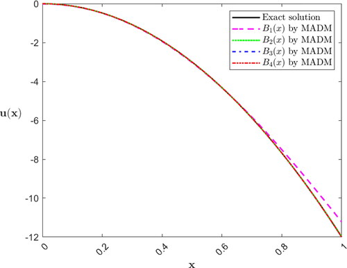
Table 1. The exact solution $u(x)=-12x^2$ of Ex. (5.1) along with the approximate solutions $B_1(x),B_2(x),B_3(x)$ and $B_4(x)$ using the MADM and the corresponding infinite norm of absolute errors in bold.

x	Exact solution	$B_1(x)$ by MADM	$\left|E_1\right|$	$B_2(x)$ by MADM	$\left|E_2\right|$	$B_3(x)$ by MADM	$\left|E_3\right|$	$B_4(x)$ by MADM	$\left|E_4\right|$
0.0	0.0	–0.0164430771	0.0164430771	$-0.0002213907$	0.0002213907	–0.0000002881	0.0000002881	0.0000000422	0.0000000422
0.2	–0.48	–0.489589233	$0.0095892332$	$-0.4801277817$	0.0001277817	–0.4800001745	0.0000001745	–0.4799999762	0.0000000237
0.4	$-1.92$	–1.9437021138	0.0237021138	$-1.9203252713$	0.0003252713	–1.9199992622	0.0000007377	–1.9199999283	0.0000000716
0.6	–4.32	–4.3272964435	0.0072964435	$-4.3210954158$	0.0010954158	–4.3200086691	0.0000086691	–4.3199998602	0.0000001397
0.8	–7.68	–7.5089686233	0.1710313766	$-7.6800848831$	0.0000848831	–7.6800484583	0.0000484583	–7.6800006026	$\mathbf{0}.\mathbf{0}\mathbf{0}\mathbf{0}\mathbf{0}\mathbf{0}\mathbf{0}\mathbf{6}\mathbf{0}\mathbf{2}\mathbf{6}$
1.0	–12.0	–11.2252109719	$\mathbf{0}.\mathbf{7}\mathbf{7}\mathbf{4}\mathbf{7}\mathbf{8}\mathbf{9}\mathbf{0}\mathbf{2}\mathbf{8}\mathbf{0}$	$-11.9791859041$	$\mathbf{0}.\mathbf{0}\mathbf{2}\mathbf{0}\mathbf{8}\mathbf{1}\mathbf{4}\mathbf{0}\mathbf{9}\mathbf{5}\mathbf{8}$	–11.9997251871	$\mathbf{0}.\mathbf{0}\mathbf{0}\mathbf{0}\mathbf{2}\mathbf{7}\mathbf{4}\mathbf{8}\mathbf{1}\mathbf{2}\mathbf{8}$	–11.9999997371	0.0000002628

(2.) Approximate solution using the HAM

The zero-order deformation is defined, from using Equation (4.6)(4.6) $$(1-q)[\Phi (x;\mathit{\hslash },q)-u_0(x)]=q\mathit{\hslash }\mathbf{N}[\Phi (x;\mathit{\hslash },q)].$$(4.6) , as below. (5.8) $$(1-q)\left[\Phi (x;\mathit{\hslash },q)-x^5\right]=q\mathit{\hslash }\mathbf{N}\left[\Phi (x;\mathit{\hslash },q)\right],$$(5.8) where $u_0(x)=x^5$ and the operator N is defined as follows. (5.9) $$\begin{array}{c}\mathbf{N}[\Phi (x;\mathit{\hslash },q)]=\Phi (x;\mathit{\hslash },q)-\frac{1}{4}(4x^5-49x^2-\frac{1}{32}(4+e^2(x^4-x))e^{-2x}+\frac{(1-9e^{-2})}{16}{e}^{2x}+\frac{3}{40})\hfill \\ +\frac{1}{4}{\int }_0^1(H(x,t)-\frac{1}{2}{\int }_0^1{\sinh }^2(x-y)M_2(y,t)dy)\Phi (t;\mathit{\hslash },q)dt,\hfill \end{array}$$(5.9) where the functions H(x, t), and $M_2(y,t)$ are defined by Equations (5.4)(5.4) $$H(x,t)=\frac{1}{32}\{\begin{array}{cc}t\left((x-1)e^{-2x+2}-32x^2\right),\hfill & \text{if}\hspace{1em}0\le t\le x,\hfill \\ (t-1)\left(x{e}^{-2x+2}-32x^2\right),\hfill & \text{if}\hspace{1em}x<t\le 1.\hfill \end{array}$$(5.4) and (5.5)(5.5) $$M_2(y,t)=\{\begin{array}{cc}t(y-1),\hfill & \text{if}\hspace{1em}0\le t\le y,\hfill \\ y(t-1),\hfill & \text{if}\hspace{1em}y\le t\le 1.\hfill \end{array}$$(5.5) respectively. It is obvious that setting p = 0, and p = 1 in Equation (5.8)(5.8) $$(1-q)\left[\Phi (x;\mathit{\hslash },q)-x^5\right]=q\mathit{\hslash }\mathbf{N}\left[\Phi (x;\mathit{\hslash },q)\right],$$(5.8) yields $\Phi (x;\mathit{\hslash },0)=x^5$ and $\Phi (x;\mathit{\hslash },1)=u(x).$ Applying the recursive Equations (4.9)(4.9) $$\begin{array}{cc}{u}_1(x)\hfill & =\mathit{\hslash }\mathbf{N}(u_0(x)).\hfill \\ u_k(x)\hfill & =u_{k-1}(x)+\frac{\mathit{\hslash }}{(k-1)!}\left[\frac{{\partial }^{k-1}}{\partial q^{k-1}}\mathbf{N}\left(\sum _{i=0}^{\infty }{u}_i(x)q^i\right)\right]{|}_{q=0},\hspace{1em}k\ge 2.\hfill \end{array}$$(4.9) gives (5.10) $$\begin{array}{c}{u}_0(x)=x^5,\\ u_1(x)=\mathit{\hslash }\left(-0.041666667x^8+12.25595238x^2-0.01930804+0.00350095e^{2x}\right)\\ +\mathit{\hslash }\left(+0.00137445x^7+0.05772700x^4-0.05910145x+0.032250164\right)e^{-2x},\\ u_2(x)=0.00115741{\mathit{\hslash }}^2{x}^{11}-\mathit{\hslash }(0.04166667+0.041666667\mathit{\hslash })x^8-1.02132937{\mathit{\hslash }}^2{x}^5\\ +0.00482701{\mathit{\hslash }}^2{x}^3+(12.25595238+12.49363864\mathit{\hslash })\mathit{\hslash }{x}^2\\ +(-0.00002673{\mathit{\hslash }}^2{x}^{10}+0.00017181{\mathit{\hslash }}^2{x}^9+0.00060132{\mathit{\hslash }}^2{x}^8\\ +(0.00137445+0.00317842\mathit{\hslash })\mathit{\hslash }{x}^7+0.011725797{\mathit{\hslash }}^2{x}^6+0.02345159{\mathit{\hslash }}^2{x}^5\\ +(0.15186267\mathit{\hslash }+0.05772700)\mathit{\hslash }{x}^4+0.02778970{\mathit{\hslash }}^2{x}^3+0.0173688{\mathit{\hslash }}^2{x}^2\\ -\mathit{\hslash }(0.11398511\mathit{\hslash }+0.05910145)x+\mathit{\hslash }(0.03225016+0.05195881\mathit{\hslash }))e^{-2x}\\ +{\mathit{\hslash }}^2(0.00001984x^7+0.00013885x^6+0.00062483x^5+0.00291586x^4\\ +0.00853929x^3+0.016870309x^2+0.02007874x+0.01210901)e^{-4x}\\ +(-0.00043762{\mathit{\hslash }}^2{x}^2+0.00350095\mathit{\hslash }+0.00697466{\mathit{\hslash }}^2)e^{2x}\\ -\mathit{\hslash }(0.01930804+0.03837772\mathit{\hslash }),\\ ⋮\end{array}$$(5.10) The values of $\mathit{\hslash }$ that ensure the convergence of the approximate solution to the exact (closed form) solution are evaluated from the line segments that are nearly parallel to the $\mathit{\hslash }-$ axis in the $\mathit{\hslash }-$ curves in Figure 2. Minimizing the squared of residual yields the optimal value of $\mathit{\hslash },$ see Figure 3. For example, minimizing the squared residual that is based on utilizing $B_1(x),B_2(x),B_3(x),B_4(x),$ where $x\in [0,1],$ gives $\mathit{\hslash }\simeq -1.035526,-1.012718,-1.004832,-1.010456,$ see Figure 3. Using $\mathit{\hslash }=-1$ gives the same results that we obtained when we utilized the MADM in Table 1. So, from the results that are obtained in Tables 1 and 2, we can notice that the two methods are very efficient in solving Ex. (5.1) and converge very fast to the exact solution under satisfying conditions of Thm. (2.3). But the HAM may converge slightly faster than the MADM when we use the optimal value of ${\mathit{\hslash }}_n$ corresponding to each $B_n(x),n=1,2,3,\dots .$

Figure 2. The $\hslash -$ curves of $u\prime (0)$ in Ex. (5.1) based on using $2\text{nd},3\text{rd}$ and $4\text{th}$ approximations in the HAM.

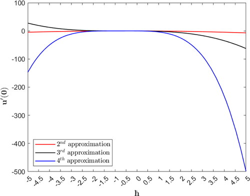
Figure 3. Depiction of the optimal value of the control parameter ${\hslash }_n$ corresponding to each $B_n(x),n=1,2,3,4$ using the HAM in Ex. (5.1).

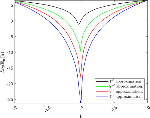
Table 2. The exact solution $u(x)=-12x^2$ of Ex. (5.1) along with the approximate solutions $B_1(x),B_2(x),B_3(x)$ and $B_4(x)$ utilizing the HAM and the corresponding infinite norm of absolute errors in bold.

		$\hslash =-1.035526$		$\hslash =-1.012718$		$\hslash =-1.004832$		$\hslash =-1.010456$
x	Exact solution	$B_1(x)$ by HAM	$\left|E_1\right|$	$B_2(x)$ by HAM	$\left|E_2\right|$	$B_3(x)$ by HAM	$\left|E_3\right|$	$B_4(x)$ by HAM	$\left|E_4\right|$
0.0	0.0	–0.0170272339	0.0170272339	0.0001965075	0.0001965075	0.0000017907	0.0000017907	–0.0000000159	0.0000000159
0.2	–0.48	–0.506993748	0.0269937486	–0.4798063482	0.0001936517	–0.4799990360	0.0000009639	$-0.4800000032$	0.0000000032
0.4	–1.92	–2.0131178612	0.0931178612	–1.9194108314	0.0005891685	–1.9199963769	0.0000036230	–1.9200000425	0.0000000425
0.6	–4.32	–4.4837904784	0.1637904784	–4.3202241764	0.0002241764	–4.3199937725	0.0000062274	–4.3200001278	0.0000001278
0.8	–7.68	–7.7873734016	0.1073734016	–7.6831975150	0.0031975150	–7.6800367880	$\mathbf{0}.\mathbf{0}\mathbf{0}\mathbf{0}\mathbf{0}\mathbf{3}\mathbf{6}\mathbf{7}\mathbf{8}\mathbf{8}\mathbf{0}$	–7.6799992887	0.0000007112
1.0	–12.0	–11.6595238159	$\mathbf{0}.\mathbf{3}\mathbf{4}\mathbf{0}\mathbf{4}\mathbf{7}\mathbf{6}\mathbf{1}\mathbf{8}\mathbf{4}\mathbf{0}$	–11.9965085659	$\mathbf{0}.\mathbf{0}\mathbf{0}\mathbf{3}\mathbf{4}\mathbf{9}\mathbf{1}\mathbf{4}\mathbf{3}\mathbf{4}\mathbf{0}$	–11.9999727632	0.0000272367	–12.0000010674	$\mathbf{0}.\mathbf{0}\mathbf{0}\mathbf{0}\mathbf{0}\mathbf{0}\mathbf{1}\mathbf{0}\mathbf{6}\mathbf{7}\mathbf{4}$

Example 5.2.

Consider the following boundary value problem (5.11) $$\begin{array}{c}{\psi }^{″}(x)-\frac{1}{64}x{e}^x{\psi }^{\prime }(x)-\frac{1}{8}\psi (x)+\frac{1}{40}{\int }_0^1\cosh (x-y){\left(\psi (y)\right)}^{2}dy=f(x),\hfill \\ 0\le x\le 1,\hspace{1em}\psi (0)=1,\hspace{1em}\psi (1)=e^{-1}.\hfill \end{array}$$(5.11)

Applying Equation (2.11)(2.11) $$\psi (x)=\frac{1}{(b-a)}\left[{\zeta }_0(b-x)+{\zeta }_1(x-a)+{\int }_a^b{M}_2(x,t)u(t)dt\right].$$(2.11) yields (5.12) $$\psi (x)=\left(1+c_{1}x+{\int }_0^1{M}_2(x,t)u(t)dt\right),$$(5.12) where $c_1:=e^{-1}-1$ and (5.13) $$\begin{array}{c}u(x)+{\int }_0^1\left(H(x,t)+\frac{1}{20}{\int }_0^1\left(1+c_{1}y\right)\cosh (x-y)M_2(y,t)dy\right)u(t)dt\hfill \\ =F(x)-\frac{1}{40}{\int }_0^1\cosh (x-y){\left({\int }_0^1{M}_2(y,t)u(t)dt\right)}^{2}dy,\hfill \end{array}$$(5.13) (5.14) $$H(x,t)=\frac{-1}{64}\{\begin{array}{cc}t\left(x{e}^x+8(x-1)\right),\hfill & \text{if}\hspace{1em}0\le t\le x,\hfill \\ x(t-1)\left(e^x+8\right),\hfill & \text{if}\hspace{1em}x<t\le 1.\hfill \end{array}$$(5.14) (5.15) $$M_2(y,t)=\{\begin{array}{cc}t(y-1),\hfill & \text{if}\hspace{1em}0\le t\le y,\hfill \\ y(t-1),\hfill & \text{if}\hspace{1em}y\le t\le 1.\hfill \end{array}$$(5.15)

The exact (closed form) solution of Equation (5.13)(5.13) $$\begin{array}{c}u(x)+{\int }_0^1\left(H(x,t)+\frac{1}{20}{\int }_0^1\left(1+c_{1}y\right)\cosh (x-y)M_2(y,t)dy\right)u(t)dt\hfill \\ =F(x)-\frac{1}{40}{\int }_0^1\cosh (x-y){\left({\int }_0^1{M}_2(y,t)u(t)dt\right)}^{2}dy,\hfill \end{array}$$(5.13) is $u(x)=e^{-x}$ with $F(x)=\frac{1}{64}(8c_1+1)x+\frac{1}{8}+\frac{1}{80}\left(c_2+\frac{5}{4}{c}_{1}x\right)e^x+\frac{1}{80}{c}_3{e}^{-x},$ where $c_2:=\frac{-2}{3}+4e^{-1}-8e^{-2}+\frac{14}{3}{e}^{-3},c_3:=78-2e-8e^{-1}+2e^{-2},.$ Applying Equation (5.12)(5.12) $$\psi (x)=\left(1+c_{1}x+{\int }_0^1{M}_2(x,t)u(t)dt\right),$$(5.12) yields $\psi (x)=e^{-x}$ with $f(x)=\frac{1}{64}x+\frac{1}{240}(1-e^{-3})e^x+\frac{1}{80}(71-e^{-1})e^{-x}.$ The kernel $K(x-y)=\cosh (x-y)$ is a real-valued continuous function in $x\forall y\in [0,1]$ and ${({\int }_0^1{\cosh }^2(x-y)dy)}^{\frac{1}{2}}\le \frac{6}{5},\forall x\in [0,1].$ Indeed, it is easy to see that $(\beta +\left|\lambda \right|(c^{*}(1)+\Lambda ))=\frac{341}{763}<\left|\mu \right|.$ Therefore, Equation (5.13)(5.13) $$\begin{array}{c}u(x)+{\int }_0^1\left(H(x,t)+\frac{1}{20}{\int }_0^1\left(1+c_{1}y\right)\cosh (x-y)M_2(y,t)dy\right)u(t)dt\hfill \\ =F(x)-\frac{1}{40}{\int }_0^1\cosh (x-y){\left({\int }_0^1{M}_2(y,t)u(t)dt\right)}^{2}dy,\hfill \end{array}$$(5.13) has a unique solution in Ω_r with $r\simeq 1.3024.$

(1.) Approximate solution using the MADM (5.16) $$\begin{array}{cc}{\widehat{u}}_0(x)\hfill & =\frac{1}{64}\left(8c_1+1\right)x,\hfill \\ {\widehat{u}}_1(x)\hfill & =\frac{1}{8}+\frac{1}{80}\left(c_2+\frac{5}{4}{c}_{1}x\right)e^x+\frac{1}{80}{c}_3{e}^{-x}\hfill \\ \hfill & -{\int }_0^1\left(H(x,t)+\frac{1}{20}{\int }_0^1\left(1+c_{1}y\right)\cosh (x-y)M_2(y,t)dy\right){\widehat{u}}_0(t)dt\hfill \\ \hfill & -\frac{1}{40}{\int }_0^1\cosh (x-y)A_0(y)dy,\hfill \\ {\widehat{u}}_m(x)\hfill & =-{\int }_0^1\left(H(x,t)+\frac{1}{20}{\int }_0^1\left(1+c_{1}y\right)\cosh (x-y)M_2(y,t)dy\right){\widehat{u}}_{m-1}(t)dt\hfill \\ \hfill & -\frac{1}{40}{\int }_0^1\cosh (x-y)A_{m-1}(y)dy,m\ge 2.\hfill \end{array}$$(5.16) Using the recursive Equation (5.16)(5.16) $$\begin{array}{cc}{\widehat{u}}_0(x)\hfill & =\frac{1}{64}\left(8c_1+1\right)x,\hfill \\ {\widehat{u}}_1(x)\hfill & =\frac{1}{8}+\frac{1}{80}\left(c_2+\frac{5}{4}{c}_{1}x\right)e^x+\frac{1}{80}{c}_3{e}^{-x}\hfill \\ \hfill & -{\int }_0^1\left(H(x,t)+\frac{1}{20}{\int }_0^1\left(1+c_{1}y\right)\cosh (x-y)M_2(y,t)dy\right){\widehat{u}}_0(t)dt\hfill \\ \hfill & -\frac{1}{40}{\int }_0^1\cosh (x-y)A_0(y)dy,\hfill \\ {\widehat{u}}_m(x)\hfill & =-{\int }_0^1\left(H(x,t)+\frac{1}{20}{\int }_0^1\left(1+c_{1}y\right)\cosh (x-y)M_2(y,t)dy\right){\widehat{u}}_{m-1}(t)dt\hfill \\ \hfill & -\frac{1}{40}{\int }_0^1\cosh (x-y)A_{m-1}(y)dy,m\ge 2.\hfill \end{array}$$(5.16) implies (5.17) $$\begin{array}{c}{\widehat{u}}_0(x)=\frac{1}{64}(8c_1+1)x,\hfill \\ {\widehat{u}}_1(x)=-0.00132063x^3+0.00132063x+0.125+0.87356526e^{-x}\hfill \\ -\left(0.00049523x^3+0.00971181x+0.00059626\right)e^x,\hfill \\ {\widehat{u}}_2(x)\hfill & =-0.00000825x^5+0.00002751x^3+0.0078125x^2+0.04643439x\hfill \\ -0.11303478+0.11071482e^{-x}+(-0.00000516x^5-0.00005159x^3\hfill \\ +0.00232455x^2+0.00518223x+0.00446825)e^x+(-0.00000774x^4+0.00002321x^3-0.00019818x^2+0.00018886x)e^{2x}\hfill \\ ⋮\hfill \end{array}$$(5.17) where Table 3 shows the absolute errors between the exact solution and the first four approximate solutions using the MADM. We can observe that the approximate solutions, that are obtained using the MADM, converge very fast to the exact solution, see Figure 4.

Figure 4. The exact (closed form) solution $u(x)=e^{-x}$ and approximate solutions $B_1(x),B_2(x),$ $B_3(x)$ and $B_4(x)$ for Ex. (5.2) using the MADM.

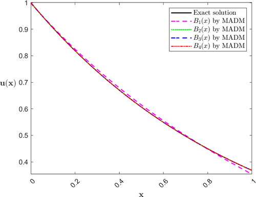
Table 3. The exact solution $u(x)=e^{-x}$ of Ex. (5.2) along with the approximate solutions $B_1(x),B_2(x),B_3(x)$ and $B_4(x)$ using the MADM and the corresponding infinite norm of absolute errors in bold.

x	Exact solution	$B_1(x)$ by MADM	$\left|E_1\right|$	$B_2(x)$ by MADM	$\left|E_2\right|$	$B_3(x)$ by MADM	$\left|E_3\right|$	$B_4(x)$ by MADM	$\left|E_4\right|$
0.0	1.0	0.9979690042	0.0020309957	$1.0001172882$	0.0001172882	1.0001029971	0.0001029971	1.0001046482	0.0001046482
0.2	0.8187307530	0.8246847756	0.0059540225	0.8187765069	$0.0000457539$	0.8188260122	0.0000952591	0.8188270652	$0.0000963122$
0.4	0.6703200460	0.6789238883	0.0086038423	0.6703374031	0.0000173570	0.6704116865	0.0000916405	0.6704125341	0.0000924881
0.6	0.5488116360	0.5549968542	0.0061852181	0.5488658005	0.0000541644	0.5489035503	0.0000919142	0.5489047520	0.0000931160
0.8	0.4493289641	0.4480039358	0.0013250283	0.4494580237	0.0001290596	0.4494256121	0.0000966480	0.4494273353	0.0000983712
1.0	0.3678794411	0.3536102192	$\mathbf{0}.\mathbf{0}\mathbf{1}\mathbf{4}\mathbf{2}\mathbf{6}\mathbf{9}\mathbf{2}\mathbf{2}\mathbf{1}\mathbf{9}$	0.3680140480	$\mathbf{0}.\mathbf{0}\mathbf{0}\mathbf{0}\mathbf{1}\mathbf{3}\mathbf{4}\mathbf{6}\mathbf{0}\mathbf{6}\mathbf{9}$	0.3679863179	$\mathbf{0}.\mathbf{0}\mathbf{0}\mathbf{0}\mathbf{1}\mathbf{0}\mathbf{6}\mathbf{8}\mathbf{7}\mathbf{6}\mathbf{7}$	0.3679881566	$\mathbf{0}.\mathbf{0}\mathbf{0}\mathbf{0}\mathbf{1}\mathbf{0}\mathbf{8}\mathbf{7}\mathbf{1}\mathbf{5}\mathbf{4}$

(2.) Approximate solution using the HAM

The zero-order deformation is defined, from using Equation (4.6)(4.6) $$(1-q)[\Phi (x;\mathit{\hslash },q)-u_0(x)]=q\mathit{\hslash }\mathbf{N}[\Phi (x;\mathit{\hslash },q)].$$(4.6) , as below. (5.18) $$(1-q)\left[\Phi (x;\mathit{\hslash },q)-\frac{1}{64}(8c_1+1)x\right]=q\mathit{\hslash }\mathbf{N}\left[\Phi (x;\mathit{\hslash },q)\right],$$(5.18) where $u_0(x)=\frac{1}{64}(8c_1+1)x$ and the operator N is defined as follows. (5.19) $$\begin{array}{c}\mathbf{N}[\Phi (x;\mathit{\hslash },q)]=\Phi (x;\mathit{\hslash },q)-\frac{1}{64}\left(8c_1+1\right)x-\frac{1}{8}-\frac{1}{80}\left(c_2-\frac{5}{4}{c}_{1}x\right)e^x-\frac{1}{80}{c}_3{e}^{-x}\hfill \\ +{\int }_0^1\left(H(x,t)+\frac{1}{20}{\int }_0^1\left(1+c_{1}y\right)\cosh (x-y)M_2(y,t)dy\right)\Phi (t;\mathit{\hslash },q)dt\hfill \\ +\frac{1}{40}{\int }_0^1\cosh (x-y){\left({\int }_0^1{M}_2(y,t)\Phi (t;\mathit{\hslash },q)dt\right)}^{2}dy,\hfill \end{array}$$(5.19) where the functions H(x, t), and $M_2(y,t)$ are defined by Equations (5.14)(5.14) $$H(x,t)=\frac{-1}{64}\{\begin{array}{cc}t\left(x{e}^x+8(x-1)\right),\hfill & \text{if}\hspace{1em}0\le t\le x,\hfill \\ x(t-1)\left(e^x+8\right),\hfill & \text{if}\hspace{1em}x<t\le 1.\hfill \end{array}$$(5.14) and (5.15)(5.15) $$M_2(y,t)=\{\begin{array}{cc}t(y-1),\hfill & \text{if}\hspace{1em}0\le t\le y,\hfill \\ y(t-1),\hfill & \text{if}\hspace{1em}y\le t\le 1.\hfill \end{array}$$(5.15) respectively. It is obvious that setting p = 0, and p = 1 in Equation (5.18)(5.18) $$(1-q)\left[\Phi (x;\mathit{\hslash },q)-\frac{1}{64}(8c_1+1)x\right]=q\mathit{\hslash }\mathbf{N}\left[\Phi (x;\mathit{\hslash },q)\right],$$(5.18) yields $\Phi (x;\mathit{\hslash },0)=\frac{1}{64}(8c_1+1)x$ and $\Phi (x;\mathit{\hslash },1)=u(x).$ Applying the recursive Equations (4.9)(4.9) $$\begin{array}{cc}{u}_1(x)\hfill & =\mathit{\hslash }\mathbf{N}(u_0(x)).\hfill \\ u_k(x)\hfill & =u_{k-1}(x)+\frac{\mathit{\hslash }}{(k-1)!}\left[\frac{{\partial }^{k-1}}{\partial q^{k-1}}\mathbf{N}\left(\sum _{i=0}^{\infty }{u}_i(x)q^i\right)\right]{|}_{q=0},\hspace{1em}k\ge 2.\hfill \end{array}$$(4.9) gives (5.20) $$\begin{array}{cc}{u}_0(x)\hfill & =\frac{1}{64}(8c_1+1)x,\hfill \\ u_1(x)\hfill & =\mathit{\hslash }(0.00132063x^3-0.00132063x-0.125-0.87356526e^{-x})+\mathit{\hslash }(0.00049523x^3+0.00971181x+0.00059626)e^x,\hfill \\ u_2(x)\hfill & =-0.00000825{\mathit{\hslash }}^2{x}^5+\mathit{\hslash }(0.00134814\mathit{\hslash }+0.00132063)x^3+0.0078125{\mathit{\hslash }}^2{x}^2\hfill \\ +\mathit{\hslash }(0.04511376\mathit{\hslash }-0.00132063)x-\mathit{\hslash }(0.125+0.23803478\mathit{\hslash })+{\mathit{\hslash }}^2(-0.00000774x^4+0.00002321x^3-0.00019818x^2+0.00018886x)e^{2x}\hfill \\ +\mathit{\hslash }(-0.00000516\mathit{\hslash }{x}^5+(0.00049523+0.00044365\mathit{\hslash })x^3+0.00232455\mathit{\hslash }{x}^2\hfill \\ +(0.00971181+0.014894032\mathit{\hslash })x+0.00059626+0.00506451\mathit{\hslash })e^x\hfill \\ -\mathit{\hslash }(0.87356526+0.76285044\mathit{\hslash })e^{-x},\hfill \\ \hfill & ⋮\hfill \end{array}$$(5.20)

The values of $\mathit{\hslash }$ that ensure the convergence of the approximate solution to the exact (closed form) solution are evaluated from the line segments that are nearly parallel to the $\mathit{\hslash }-$ axis in the $\mathit{\hslash }-$ curves in Figure 5. Minimizing the squared of residual yields the optimal value of $\mathit{\hslash },$ see Figure 6. For example, minimizing the squared residual that is based on utilizing $B_1(x),B_2(x),B_3(x),B_4(x),$ where $x\in [0,1],$ gives $\mathit{\hslash }\simeq -0.995435,-0.996601,-0.993321,-0.993270,$ see Figure 6. Using $\mathit{\hslash }=-1$ gives the same results that we obtained when we utilized the MADM in Table 3. So, from the results that are obtained in Tables 3 and 4, we can notice that the two methods are very efficient in solving Ex. (5.2) and converge very fast to the exact solution under satisfying conditions of Thm. (2.3). But the HAM may converge slightly faster than the MADM when we use the optimal value of ${\mathit{\hslash }}_n$ corresponding to each $B_n(x),n=1,2,3,\dots .$

Figure 5. The $\hslash -$ curves of $u\prime (0)$ in Ex. (5.2) based on using $2^{nd},3^{rd}$ and $4^{th}$ approximations in the HAM.

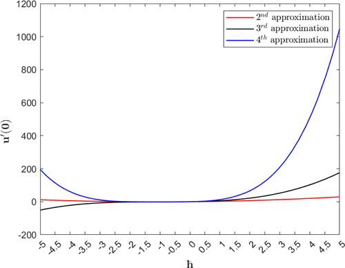
Figure 6. Depiction of the optimal value of the control parameter ${\hslash }_n$ corresponding to each $B_n(x),n=1,2,3,4$ using the HAM in Ex. (5.2).

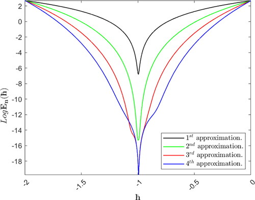
Table 4. The exact solution $u(x)=e^{-x}$ of Ex. (5.2) along with the approximate solutions $B_1(x),B_2(x),B_3(x)$ and $B_4(x)$ utilizing the HAM and the corresponding infinite norm of absolute errors in bold.

		$\hslash =-0.995435$		$\hslash =-0.996601$		$\hslash =-0.993321$		$\hslash =-0.993270$
x	Exact solution	$B_1(x)$ by HAM	$\left|E_1\right|$	$B_2(x)$ by HAM	$\left|E_2\right|$	$B_3(x)$ by HAM	$\left|E_3\right|$	$B_4(x)$ by HAM	$\left|E_4\right|$
0.0	1.0	0.9934135307	0.0065864692	1.0000911832	0.0000911832	1.0000010937	0.0000010937	1.0000008495	0.0000008495
0.2	0.8187307530	0.8208624284	0.0021316753	$0.8188069267$	0.0000761737	0.8187263177	0.0000044353	0.8187261289	0.0000046240
0.4	0.6703200460	0.6757090305	0.0053889844	0.6703875338	0.0000674878	0.6703118622	0.0000081837	0.6703117099	0.0000083361
0.6	0.5488116360	0.5522898197	$0.0034781836$	0.5489005543	0.0000889182	0.5488135983	0.0000019623	0.5488133433	0.0000017072
0.8	0.4493289641	0.4457274247	0.0036015393	0.4494423960	$\mathbf{0}.\mathbf{0}\mathbf{0}\mathbf{0}\mathbf{1}\mathbf{1}\mathbf{3}\mathbf{4}\mathbf{3}\mathbf{1}\mathbf{9}$	0.4493414172	0.0000124531	0.4493409956	0.0000120314
1.0	0.3678794411	0.3517067194	$\mathbf{0}.\mathbf{0}\mathbf{1}\mathbf{6}\mathbf{1}\mathbf{7}\mathbf{2}\mathbf{7}\mathbf{2}\mathbf{1}\mathbf{6}$	0.3679114905	0.0000320494	0.3678474836	$\mathbf{0}.\mathbf{0}\mathbf{0}\mathbf{0}\mathbf{0}\mathbf{3}\mathbf{1}\mathbf{9}\mathbf{5}\mathbf{7}\mathbf{5}$	0.3678472765	$\mathbf{0}.\mathbf{0}\mathbf{0}\mathbf{0}\mathbf{0}\mathbf{3}\mathbf{2}\mathbf{1}\mathbf{6}\mathbf{4}\mathbf{6}$

6. Conclusion

In this work, we have studied a boundary value problem for a nonlinear integro-differential equation. An equivalent NFIE has been derived for the proposed problem, then the Krasnosel’skii fixed point has been applied to investigate the existence of continuous solutions. Moreover, the sufficient conditions which guarantee the uniqueness of the solution are proved. We have determined an approximate solution to the NFIE using the MADM. The convergence and error estimates of this approximate solution are studied as well. After that, the homotopy analysis technique is applied to get another approximate solution for the NFIE. We compared the accuracy and convergence rate of the approximate solution using the two techniques. It turns out for us that both methods are efficient and converge very rapidly, but the HAM may converge slightly faster when we succeed in choosing the optimal homotopy control parameter. We may study the fractal version that is corresponding to Equation (1.1)(1.1) $$\begin{array}{c}\mu \frac{d^2\psi (x)}{d{x}^2}+A_1(x)\frac{d\psi (x)}{dx}+A_2(x)\psi (x)\hfill \\ -\lambda {\int }_a^{b}K(x-y){[\psi (y)]}^{p}dy=f(x),\hspace{1em}a\le x\le b.\hfill \end{array}$$(1.1) for future suggested work (He, 2020a, 2020b).

Authors’ contributions

The authors conducted the current research article equally and approved the submitted manuscript.

Availability of data and materials

All the needed data are enclosed in the current article.

Geolocation information

Latitude: 21.5908352

Longitude: 39.159398399999986

Acknowledgments

The authors thank the anonymous referees for their valuable comments.

Disclosure statement

The authors affirm that there are no competing interests.

Funding

Not applicable.

References

- Abdou, M. A., Soliman, A. A., & Abdel-Aty, M. A. (2020). On a discussion of Volterra–Fredholm integral equation with discontinuous kernel. Journal of the Egyptian Mathematical Society, 28(1), 11. doi:https://doi.org/10.1186/s42787-020-00074-8
- Adomian, G. (1994). Solving frontier problems of physics: The decomposition method. Kluwer Academic Publishers, Boston.
- Alhendi, F., Shammakh, W., & Al-Badrani, H. (2017). Numerical solutions for quadratic integro-differential equations of fractional orders. Open Journal of Applied Sciences, 7(4), 157–170. doi:https://doi.org/10.4236/ojapps.2017.74014
- Alidema, A., & Georgieva, A. (2018). Adomian decomposition method for solving two-dimensional nonlinear Volterra fuzzy integral equations. AIP Conference Proceedings, 2048:050009.
- Bakodah, H. O., Al-Mazmumy, M., & Almuhalbedi, S. O. (2019). Solving system of integro differential equations using discrete Adomian decomposition method. Journal of Taibah University for Science, 13(1), 805–812. doi:https://doi.org/10.1080/16583655.2019.1625189
- Elborai, M. M., Abdou, M. A., & Youssef, M. I. (2013). On Adomian’s decomposition method for solving nonlocal perturbed stochastic fractional integrodifferential equations. Life Science Journal, 10(4), 550–555.
- Hamoud, A. A., & Ghadle, K. P. (2018). The approximate solutions of fractional Volterra-Fredholm integro-differential equations by using analytical techniques. Issues of Analysis, 25(1), 41–58. doi:https://doi.org/10.15393/j3.art.2018.4350
- Hamoud, A., Ghadle, K., & Atshan, S. (2019). The approximate solutions of fractional integro-differential equations by using modified Adomian decomposition method. Khayyam Journal of Mathematics, 5(1), 21–39.
- He, J. H. (2020a). A simple approach to Volterra-Fredholm integral equations. Journal of Applied and Computational Mechanics, 6(Special Issue), 1184–1186.
- He, J. H. (2020b). A short review on analytical methods for to a fully fourth-order nonlinear integral boundary value problem with fractal derivatives. International Journal of Numerical Methods for Heat & Fluid Flow, 30(11), 4933–4943. doi:https://doi.org/10.1108/HFF-01-2020-0060
- Hetmaniok, E., Słota, D., Trawiński, T., & Wituła, R. (2014). Usage of the homotopy analysis method for solving the nonlinear and linear integral equations of the second kind. Numerical Algorithms, 67(1), 163–185. doi:https://doi.org/10.1007/s11075-013-9781-0
- Issa, M., Hamoud, A., & Ghadle, K. (2021). Numerical solutions of Fuzzy integro-differential equations of the second kind. Journal of Mathematics and Computer Science, 23, 67–74.
- Kurt, A., & Tasbozan, O. (2019). Approximate analytical solutions to conformable modified Burgers equation using homotopy analysis method. Annales Mathematicae Silesianae, 33(1), 159–167. doi:https://doi.org/10.2478/amsil-2018-0011
- Liao, S. J. (2003). Beyond perturbation introduction to the homotopy analysis method. Chapman and Hall/CRC, Boca Raton.
- Liao, S. J. (2012). Homotopy analysis method in nonlinear differential equation. Beijing: Higher Education Press and Berlin/Heidelberg: Springer-Verlag.
- Maitama, S., & Zhao, W. (2019). Local fractional homotopy analysis method for solving non-differentiable problems on Cantor sets. Advances in Difference Equations, 2019(1), 22. doi:https://doi.org/10.1186/s13662-019-2068-6
- Mirzaee, F., & Alipour, S. (2019). Numerical solution of nonlinear partial quadratic integro-differential equations of fractional order via hybrid of block-pulse and parabolic functions. Numerical Methods for Partial Differential Equations, 35(3), 1134–1151. doi:https://doi.org/10.1002/num.22342
- Rezabeyk, S., Abbasbandy, S., & Shivanian, E. (2020). Solving fractional-order delay integro-differential equations using operational matrix based on fractional-order Euler polynomials. Mathematical Sciences, 14(2), 97–107. doi:https://doi.org/10.1007/s40096-020-00320-1
- Saeedi, L., Tari, A., & Babolian, E. (2020). A study on functional fractional integro-differential equations of Hammerstein type. Computational Methods for Differential Equations, 8(2020), 173–193.
- Singh, J., Kumar, D., Baleanu, D., & Rathore, S. (2018). An efficient numerical algorithm for the fractional Drinfeld–Sokolov–Wilson equation. Applied Mathematics and Computation, 335(C), 12–24. doi:https://doi.org/10.1016/j.amc.2018.04.025
- Singh, R. R., Nelakanti, G., & Kumar, J. (2014). Approximate solution of Urysohn integral equations using the Adomian decomposition method. TheScientificWorldJournal, 2014, 150483. doi:https://doi.org/10.1155/2014/150483
- Wazwaz, A. (2010). The variational iteration method for solving linear and nonlinear Volterra integral and integro-differential equations. International Journal of Computer Mathematics, 87(5), 1131–1141. doi:https://doi.org/10.1080/00207160903124967
- Wazwaz, A. M. (1999). A reliable modification of Adomian decomposition method. Applied Mathematics and Computation, 102(1), 77–86. doi:https://doi.org/10.1016/S0096-3003(98)10024-3