Almon-KL estimator for the distributed lag model

Abstract

The Almon technique is widely used to estimate the parameters of the distributed lag model (DLM). The technique suffers a setback from the challenge of multicollinearity because the explanatory variables and their lagged values are often correlated. The Almon-Ridge estimator (A-RE) and Almon-Liu estimator (A-LE) were introduced as alternative estimators for efficient modelling. We developed a new method of estimating the coefficients of the DLM using the Almon-KL estimator (A-KLE). A-KLE dominates the other estimators considered in this study via theoretical findings, simulation design and two numerical examples. The estimators’ performance was compared using the mean squared error.

Keywords:

• Almon estimator
• Almon-Ridge
• Almon-Liu
• Almon-KL
• distributed lag model
• MSE
• multicollinearity

AMS SUBJECT CLASSIFICATION:

• 62J05
• 62J99

1. Introduction

Distributed lag model (DLM) is a model that is commonly adopted to predict the current values of a response variable based on both the current values of a regressor (explanatory variable) and its lagged values (Cromwell, Hannan, Labys, & Terraza, 1994; Judge, Griffiths, Hill, & Lee, 1980). For instance, the effect of public investment such as road and highways construction on growth in the gross national product (GNP) will show up with a lag, and this effect will likely linger on for some years (Maddala, 1974). Under certain assumptions, the ordinary least squares estimator (OLSE) is the easiest method of estimating the distributed lags’ parameters. The assumptions include assuming a fixed maximum lag; the error should be normally distributed and unrestricted relationship among the lagged explanators. However, multicollinearity arises from the relationship between the explanatory variables and their lagged explanators, resulting in a large variance of the coefficient estimates. The OLSE becomes inefficient when there is multicollinearity. Also, the method suffers a breakdown when the number of observations does not sufficiently exceed the number of lags (Almon, 1965; Fisher, 1937; Frost, 1975; Maddala, 1974). Almon technique proposed by Almon (Fisher, 1937) is widely used to estimate the parameters of DLM because the methods reduced the effect of multicollinearity (Fair & Jaffee, 1971; Majid, Aslam, Altaf, & Amanullah, 2019). The assumption under the Almon lag model is that there must be a finite lag length and the lag weight approximated by a polynomial of suitable degree.

The Almon estimator (AE) is the best linear unbiased estimator (BLUE) for the DLMs (Vinod & Ullah, 1981). Therefore, this estimator has widespread usage in applied econometrics due to its ease of estimation. However, the estimator still suffers a breakdown when there is a high correlation among the explanatory variables. Biased estimators were developed as alternatives to the OLS estimator in the linear regression model (LRM) (Baye & Parker, 1984; Hoerl & Kennard, 1970; Kaçıranlar & Sakallıoğlu, 2001; Kibria & Lukman, 2020; Li & Yang, 2012; Liu, 1993; Lukman, Ayinde, Kibria, & Adewuyi, 2020; Massy, 1965; Swindel, 1976). Some of these estimators have been adapted to AE to mitigate the effect of multicollinearity.

The ridge estimator was suggested as an alternative to the AE (Chanda & Maddala, 1984; Lindley & Smith, 1972; Lukman, Ayinde, Binuomote, & Onate, 2019; Maddala, 1974; Vinod & Ullah, 1981; Yeo & Trivedi, 2009). The limitation of the ridge regression estimator for the DLMs was pointed out in the following study (Lindley & Smith, 1972; Maddala, 1974; Yeo & Trivedi, 2009). According to Maddala (1974) and Yeo and Trivedi (2009), the empirical findings do not fulfil expectations despite adopting different ridge parameters, k. Alternative estimators include the Almon modified ridge and Liu estimators (Gültay & Kaçıranlar, 2015). Özbay & Kaçıranlar (2017) introduced the Almon two-parameter estimator to deal with the problem of multicollinearity for the DLM. The estimator extends the two-parameter estimation procedure by Özkale and Kaçıranlar (2007) to the DLM. The Almon two-parameter ridge was also developed to handle multicollinearity in DLM (Lipovetsky, 2006; Lipovetsky & Conklin, 2005; Ozbay, 2019). Kibria and Lukman (2020) developed the Kibria–Lukman estimator (KLE) to cushion the effect of multicollinearity in the LRM. The estimator gain advantage over the ridge and the Liu estimator. Thus, the focus of this study is to develop the Almon-KL estimator (A-KLE) based on KLE.

The other part of the article is structured as follows: we introduced the DLM, its estimation methods, and the proposed estimator in Section 2. Section 3 deals with the theoretical comparisons and the choice of biasing parameters. We examined the estimators’ performance using a simulation study and two examples in Sections 4 and 5, respectively. Finally, we provide a concluding remark.

2. Distributed lag model (DLM) and method of estimation

The finite DLM is defined as (2.1) $$\begin{array}{c}{y}_t={\beta }_0{x}_t+{\beta }_1{x}_{t-1}+{\beta }_2{x}_{t-2}+\dots +{\beta }_p{x}_{t-p}+u_t\\ =\sum _{i=0}^p{\beta }_i{x}_{t-i}+u_t,t=p+1,\dots ,T,\end{array}$$(2.1) where ${\beta }_i$ are the current and lagged coefficients of $x_t,$ $y_t$ denotes the t-th observation on the response variable $y,$ $x_{t-p}$ denotes the (t-p)th observation on the explanatory variable $x,$ $u_t$ is the disturbance term corresponding to the t-th observation and is assumed to be IN(0, ${\sigma }^2$) and p denotes the lag length. Model (2.1)(2.1) $$\begin{array}{c}{y}_t={\beta }_0{x}_t+{\beta }_1{x}_{t-1}+{\beta }_2{x}_{t-2}+\dots +{\beta }_p{x}_{t-p}+u_t\\ =\sum _{i=0}^p{\beta }_i{x}_{t-i}+u_t,t=p+1,\dots ,T,\end{array}$$(2.1) can be written in matrix form as (2.2) $$y=X\beta +u,$$(2.2) where $$X=\left[\begin{array}{cccc}{x}_{p+1}& x_p& \cdots & x_1\\ x_{p+2}& x_{p+1}& \cdots & x_2\\ ⋮& ⋮& \ddots & ⋮\\ x_T& x_{T-1}& \cdots & x_{T-p}\end{array}\right],y=\left(\begin{array}{c}{y}_{p+1}\\ y_{p+2}\\ ⋮\\ y_T\end{array}\right),\beta =\left[\begin{array}{c}{\beta }_0\\ {\beta }_1\\ ⋮\\ {\beta }_p\end{array}\right]\text{and}u=\left(\begin{array}{c}{u}_{p+1}\\ u_{p+2}\\ ⋮\\ u_T\end{array}\right).$$

The OLSE of $\beta$ is (2.3) $$\widehat{\beta }={\left(X^{\prime }X\right)}^{-1}{X}^{\prime }y.$$(2.3)

The OLS estimator of $\beta$ is BLUE when there is no violation of the model assumptions (Lukman et al., 2019). As earlier mentioned, there is high tendency of multicollinearity among the regressors since lags of the same explanatory variable appear in the model (Güler, Gültay, & Kaçiranlar, 2015; Gültay & Kaçıranlar, 2015). It becomes difficult to estimate with the conventional OLS when the lag length (p) is known and large (Güler et al., 2015; Gültay & Kaçıranlar, 2015; Ozbay, 2019; Özbay & Kaçıranlar, 2017). The Almon polynomial lag distribution was recommended as a replacement to the OLS estimator (Almon, 1965). The Almon polynomial lag is defined as (2.4) $${\beta }_i={\alpha }_0+{\alpha }_{1}i+{\alpha }_2{i}^2+\dots +{\alpha }_s{i}^s,p\ge s\ge 0.$$(2.4)

The above equation can simply be written as (2.5) $$\beta =A\alpha ,$$(2.5) where $\alpha =\left[\begin{array}{c}{\alpha }_0\\ {\alpha }_1\\ ⋮\\ {\alpha }_s\end{array}\right]$ and $A=\left[\begin{array}{cccc}1& 0& 0& \begin{array}{cc}\cdots & 0\end{array}\\ 1& 1& 1& \begin{array}{cc}\cdots & 1\end{array}\\ 1& 2& 2^2& \begin{array}{cc}\cdots & 2^s\end{array}\\ \begin{array}{c}⋮\\ 1\end{array}& \begin{array}{c}⋮\\ p\end{array}& \begin{array}{c}⋮\\ p^2\end{array}& \begin{array}{cc}\begin{array}{c}⋮\\ ⋮\end{array}& \begin{array}{c}⋮\\ p^s\end{array}\end{array}\end{array}\right]$ are $\alpha :(s+1)\times 1$ vector and $A:(p+1)\times (r+1)$ matrix, respectively. The ranks of matrices $X$ and $A$ are assumed to be $(p+1)<(T-p)$ and $(s+1)<(p+1),$ respectively. If $s<p$ then the rank of A is s + 1. We substitute (2.5)(2.5) $$\beta =A\alpha ,$$(2.5) into (2.2)(2.2) $$y=X\beta +u,$$(2.2) and obtained the new equation as, (2.6) $$y=XA\alpha +u=Z\alpha +u,$$(2.6) where $Z=XA.$ The OLS estimator of (2.6)(2.6) $$y=XA\alpha +u=Z\alpha +u,$$(2.6) becomes the AE in (2.7)(2.7) $${\widehat{\alpha }}_A={\left(Z^{\prime }Z\right)}^{-1}{Z}^{\prime }y,$$(2.7) : (2.7) $${\widehat{\alpha }}_A={\left(Z^{\prime }Z\right)}^{-1}{Z}^{\prime }y,$$(2.7) such that (2.8) $${\widehat{\beta }}_A=A{\widehat{\alpha }}_A.$$(2.8)

Equation (2.8)(2.8) $${\widehat{\beta }}_A=A{\widehat{\alpha }}_A.$$(2.8) is referred to as AE of $\beta$ which is still BLUE. A notable problem with this technique centered on the choice of lag length and the degree of the polynomial, respectively because the two are unknown in practice. One of the suggested means of selecting the lag length is to select a reasonable lag and check if it fit the model (2.1)(2.1) $$\begin{array}{c}{y}_t={\beta }_0{x}_t+{\beta }_1{x}_{t-1}+{\beta }_2{x}_{t-2}+\dots +{\beta }_p{x}_{t-p}+u_t\\ =\sum _{i=0}^p{\beta }_i{x}_{t-i}+u_t,t=p+1,\dots ,T,\end{array}$$(2.1) using any of the following criteria: Akaike information criterion (AIC), Bayesian information criterion (BIC) and adjusted coefficient of determination $({\overline{R}}^2)$ (Davidson & MacKinnon, 1993). The ridge estimator was suggested as an alternative approach due to the limitation of the AE. The Almon-Ridge estimator (A-RE) of $\beta$ is defined as (2.9) $${\widehat{\beta }}_A^k=A{\widehat{\alpha }}^k,k>0$$(2.9) where ${\widehat{\alpha }}^k={(Z^{\prime }Z+kI)}^{-1}{Z}^{\prime }y.$ Özbay and Toker (2021) examined the predictive performance of A-RE. According to Gültay & Kaçıranlar (2015), the Almon-Liu estimator (A-LE) is defined as: (2.10) $${\widehat{\beta }}_A^d=A{\widehat{\alpha }}^d,\left(0\mathrm{ }<\mathrm{d}\mathrm{ }<1\right)$$(2.10) where ${\widehat{\alpha }}^d={(Z^{\prime }Z+I)}^{-1}(Z^{\prime }Z+dI){\widehat{\alpha }}_A.$

The Liu estimator overcomes the limitation in the ridge estimator for the LRM. Recently, Kibria and Lukman (2020) developed the KL estimator (KLE) to mitigate multicollinearity in the LRM. The estimator is a modification of the Liu estimator; it gained an advantage over the Liu estimator using the mean squared error. The bias of KLE is two times lower than the bias of the ridge estimator. Thus, the KL estimator performs better than the ridge and the Liu estimators. Following this merit, the estimator is adapted to the AE to handle multicollinearity in this study. The A-KLE is defined as (2.11) $${\widehat{\beta }}_A^{KL}=A{\widehat{\alpha }}^{KL},$$(2.11) where ${\widehat{\alpha }}^{KL}={(Z^{\prime }Z+kI)}^{-1}(Z^{\prime }Z-kI){\widehat{\alpha }}_A.$

Suppose $Z=XQ,\alpha =Q^{\prime }\beta ,$ and $Z^{\prime }Z=Q^{\prime }{X}^{\prime }XQ=E=\mathit{diag}(e_1,\dots ,e_{s+1})$ such that $e_1\ge e_2\ge \dots \ge e_{s+1}$ are the ordered eigenvalues of $Z^{\prime }Z$ and $Q$ is the matrix whose columns are the eigenvectors of $Z^{\prime }Z.$ and the canonical form of the estimators are as follows: (2.12) $${\widehat{\alpha }}_A=E^{-1}{Z}^{\prime }y,$$(2.12) (2.13) $${\widehat{\alpha }}^k={\left(E+kI\right)}^{-1}{Z}^{\prime }y,$$(2.13) (2.14) $${\widehat{\alpha }}^d={\left(E+I\right)}^{-1}\left(E+dI\right){\widehat{\alpha }}_A,$$(2.14) (2.15) $${\widehat{\alpha }}^{KL}={\left(E+kI\right)}^{-1}\left(E-kI\right){\widehat{\alpha }}_A.$$(2.15)

The statistical properties of A-KLE are as follows:

The bias of the A-KLE is defined as: (2.16) $$B({\widehat{\alpha }}^{KL})=-2k{E}^k\alpha ,$$(2.16) where $E^k={(E+kI)}^{-1}.$ The variance of the A-KLE is defined as: (2.17) $$D({\widehat{\alpha }}^{KL})={\sigma }^2{E}^k(E-kI)E^{-1}{E}^k(E-kI).$$(2.17)

Therefore, the mean square error matrix (MSEM) and the scalar mean square error (SMSE) of A-KLE, respectively, are (2.18) $$\mathit{MSEM}({\widehat{\alpha }}^{KL})={\sigma }^2{E}^k(E-kI)E^{-1}{E}^k(E-kI)+4k^2{E}^k{E}^k\alpha {\alpha }^{\prime },$$(2.18) and (2.19) $$\mathit{SMSE}({\widehat{\alpha }}^{KL})={\sigma }^2\sum _{i=1}^{s+1}\left(\frac{{\left(e_i-k\right)}^2}{e_i{\left(e_i+k\right)}^2}\right)+4k^2\sum _{i=1}^{s+1}\left(\frac{{\alpha }_i^2}{{\left(e_i+k\right)}^2}\right).$$(2.19)

3. Theoretical comparisons among the estimators

In this section, we adopted Lemma 3.1 to evaluate the estimators’ performance.

Lemma 3.1.

Let ${\widehat{\beta }}_1$ and ${\widehat{\beta }}_2$ be two linear estimators of $\beta .$ The difference in the covariance of the two estimators $D$ is positive definite if and only if $\mathit{bias}{({\widehat{\beta }}_2)}^{\prime }{\left[{\sigma }^{2}D+\mathit{bias}({\widehat{\beta }}_1)b\mathit{ias}{({\widehat{\beta }}_1)}^{\prime }\right]}^{-1}b\mathit{ias}({\widehat{\beta }}_2)<1.$

Consequently, $$\mathit{MSEM}({\widehat{\beta }}_1)-\mathit{MSEM}({\widehat{\beta }}_2)={\sigma }^{2}D+\mathit{bias}({\widehat{\beta }}_1)\mathit{bias}({\widehat{\beta }}_1{)}^{\prime }-\mathit{bias}({\widehat{\beta }}_2)\mathit{bias}({\widehat{\beta }}_1{)}^{\prime }>0$$

(R Core Team, 2020; Trenkler & Toutenburg, 1990).

3.1. Comparison between ${\widehat{\alpha }}_A$ and ${\widehat{\alpha }}^{KL}$

Theorem 3.1.

The estimator ${\widehat{\alpha }}^{KL}$ is preferred to ${\widehat{\alpha }}_A$ in the MSEM sense, if and only if, $b^{\prime }{[{\sigma }^2(E^{-1}-E^k(E-kI)E^{-1}{E}^k(E-kI))]}^{-1}b<1$ where $b=-2k{E}^k\alpha .$

Proof.

(3.1) $$\begin{array}{c}D\left({\widehat{\tilde{\alpha }}}_A\right)-D\left({\widehat{\alpha }}^{KL}\right)=\left[{\sigma }^2{E}^{-1}-{\sigma }^2{E}^k(E-kI)E^{-1}{E}^k(E-kI)\right]\\ ={\sigma }^{2}d\mathit{iag}{\left\{\frac{1}{e_i}-\frac{{\left(e_i-k\right)}^2}{e_i{\left(e_i+k\right)}^2}\right\}}_{i=1}^{s+1}.\end{array}$$(3.1)

It is noted that $E^{-1}-E^k(E-kI)E^{-1}{E}^k(E-kI)$ is non-negative (nn) because $e_i+k>e_i-k$ for $k>0.$

3.2. Comparison between ${\widehat{\alpha }}^k$ and ${\widehat{\alpha }}^{KL}$

Theorem 3.2.

The estimator ${\widehat{\alpha }}^{KL}$ is preferred to ${\widehat{\alpha }}^k$ in the MSEM sense, if and only if, $b^{\prime }{[{\sigma }^2(E^{k}E{E}^k-E^k(E-kI)E^{-1}{E}^k(E-kI))+{\widetilde{b^{\prime }}}_1{b}_1]}^{-1}b<1$ where $b=-2k{E}^k\alpha$ and $b_1=k{E}^k\alpha .$

Proof.

(3.2) $$\begin{array}{c}D\left({\widehat{\alpha }}^k\right)-D\left({\widehat{\alpha }}^{KL}\right)=\left[{\sigma }^2\left(E^{k}E{E}^k-E^k(E-kI)E^{-1}{E}^k(E-kI)\right)\right]\\ ={\sigma }^{2}d\mathit{iag}{\left\{\frac{e_i}{{\left(e_i+k\right)}^2}-\frac{{\left(e_i-k\right)}^2}{e_i{\left(e_i+k\right)}^2}\right\}}_{i=1}^{s+1}.\end{array}$$(3.2)

It is noted that $E^{k}E{E}^k-E^k(E-kI)E^{-1}{E}^k(E-kI)$ is non-negative because $e_i^2-{(e_i-k)}^2>0$ for $k<2e_i.$

3.3. Comparison between ${\widehat{\alpha }}^d$ and ${\widehat{\alpha }}^{KL}$

Theorem 3.3.

The estimator ${\widehat{\alpha }}^{KL}$ is preferred to ${\widehat{\alpha }}^d$ in MSEM sense if and only if, $b^{\prime }{[{\sigma }^2(E_d{E}^{-1}{E^{\prime }}_d-E^k(E-kI)E^{-1}{E}^k(E-kI))+{b^{\prime }}_2{b}_2]}^{-1}b<1$ where $b=-2k{E}^k\alpha$ and ${\tilde{b}}_2=-(1-d){(E+I)}^{-1}\alpha .$

Proof.

(3.3) $$\begin{array}{c}D\left({\widehat{\alpha }}^d\right)-D\left({\widehat{\alpha }}^{KL}\right)=\left[{\sigma }^2\left(E_d{E}^{-1}{E^{\prime }}_d-E^k(E-kI)E^{-1}{E}^k(E-kI)\right)\right]\\ ={\sigma }^{2}d\mathit{iag}{\left\{\frac{{\left(e_i+d\right)}^2}{e_i{\left(e_i+1\right)}^2}-\frac{{\left(e_i-k\right)}^2}{e_i{\left(e_i+k\right)}^2}\right\}}_{i=1}^{s+1}.\end{array}$$(3.3)

It is noted that $E_d{E}^{-1}{E^{\prime }}_d-E^k(E-kI)E^{-1}{E}^k(E-kI)$ is non-negative since ${(e_i+k)}^2{(e_i+d)}^2-{(e_i-k)}^2{(e_i+1)}^2>0$ for $k>\frac{e_i(1-d)}{d+e_i+1}$ and $d>\frac{e_i(1-k)-k}{e_i+k}.$

4. Monte Carlo simulation study

We conducted a simulation study for DLM to explore the estimators’ performance. The dependent variable and explanatory variables are generated according to the following study (Güler et al., 2015; Özbay & Kaçıranlar, 2017; Özbay & Toker, 2021). (4.1) $$y_t={\beta }_0{x}_t+{\beta }_1{x}_{t-1}+\dots {\beta }_p{x}_{t-p}+u_t,$$(4.1) (4.2) $$x_1=v_1,$$(4.2) (4.3) $$x_t=\tau x_{t-1}+\sqrt{1-{\tau }^2}{v}_t\forall t\ge 2,$$(4.3) where$\tau$ denotes the correlation between the regressors and its values are chosen as follows: 0.8, 0.9, 0.99, and 0.999. The MSE is minimized subject to the constraint ${\beta }^{\prime }\beta =1$ (Güler et al., 2015; Özbay & Kaçıranlar, 2017; Özbay & Toker, 2021). $u_t$ and $v_t$ are generated such that $u_t\sim N(0,{\sigma }^2)$ and $v_t\sim N(0,1),$ respectively. The choices of ${\sigma }^2$ are 1, 5 and 10. The data for each replication are determined in accordance with the following studies (Güler et al., 2015; Özbay & Kaçıranlar, 2017; Özbay & Toker, 2021). An observation of T-p = 60 and 100 with the lag length of 8 and 16 was evaluated. The experiment is repeated 2000 times using the RStudio programming language (R Core Team, 2020). The model (4.1) is transformed back to the Almon model (2.6)(2.6) $$y=XA\alpha +u=Z\alpha +u,$$(2.6) after generating the observations. The mean squared error is obtained as follows: (4.4) $$\mathit{MSE}\left(\widehat{\beta }\right)=\frac{1}{2000}\sum _{j=1}^{2000}{\left({\widehat{\beta }}_{ij}-{\beta }_i\right)}^{\prime }\left({\widehat{\beta }}_{ij}-{\beta }_i\right)$$(4.4) where ${\widehat{\beta }}_{ij}$ denotes the estimate of the ith parameter in jth replication and ${\beta }_i$ is the true parameter values. The simulated MSE values are presented in Tables 1 and 2 for lag length are 8 and 16, respectively.

Table 1. Estimated MSE’s when lag length is 8.

$\mathrm{\tau }$	n	${\widehat{\alpha }}_A$	${\widehat{\alpha }}^k$	${\widehat{\alpha }}^d$	${\widehat{\alpha }}^{KL}$	${\widehat{\alpha }}_A$	${\widehat{\alpha }}^k$	${\widehat{\alpha }}^d$	${\widehat{\alpha }}^{KL}$
		$\sigma =1$				$\sigma =3$
0.8	60	0.1674	0.1602	0.1650	0.1592	0.6916	0.4321	0.6715	0.4218
	100	0.0868	0.0822	0.0859	0.0817	0.3625	0.2501	0.3570	0.2471
0.9	60	0.2100	0.1839	0.2026	0.1803	1.1223	0.5994	1.0569	0.5656
	100	0.1150	0.1040	0.1126	0.1026	0.5820	0.3468	0.5644	0.3376
0.99	60	0.9213	0.5185	0.6491	0.4089	7.8423	3.2830	5.2921	2.1330
	100	0.5481	0.3218	0.4303	0.2708	4.5558	1.9046	3.4994	1.4332
0.999	60	8.1325	3.2601	2.2957	1.8764	72.8119	27.1628	19.4490	13.1906
	100	4.7814	1.9103	1.5831	1.1510	42.8105	15.4087	13.5760	7.4965
		$\sigma =5$				$\sigma =10$
0.8	60	1.7403	0.9165	1.6845	0.8882	6.6563	3.1017	6.4333	2.9896
	100	0.9136	0.5319	0.8989	0.5244	3.4961	1.7298	3.4387	1.7015
0.9	60	2.9472	1.3722	2.7656	1.2797	11.5020	4.9011	10.7757	4.5334
	100	1.5155	0.7646	1.4678	0.7408	5.8904	2.5921	5.7016	2.5005
0.99	60	21.6850	8.6932	14.5764	5.4667	86.5740	34.0261	58.0927	21.0607
	100	12.5698	4.9479	9.6402	3.6427	50.1325	19.1852	38.4314	13.9808
0.999	60	202.1728	74.9526	53.7505	35.7999	808.5568	298.9995	214.5284	141.7912
	100	118.8650	42.3641	37.5870	20.1206	475.3627	168.7284	150.1936	79.2424

Table 2. Estimated MSE’s when lag length is 16.

$\mathrm{\tau }$	n	${\widehat{\alpha }}_A$	${\widehat{\alpha }}^k$	${\widehat{\alpha }}^d$	${\widehat{\alpha }}^{KL}$	${\widehat{\alpha }}_A$	${\widehat{\alpha }}^k$	${\widehat{\alpha }}^d$	${\widehat{\alpha }}^{KL}$
		$\sigma =1$				$\sigma =3$
0.8	60	0.2962	0.2972	0.2958	0.2871	0.4960	0.4843	0.4944	0.4837
	100	0.2683	0.2671	0.2681	0.2670	0.4060	0.3863	0.4053	0.3859
0.9	60	0.3338	0.3369	0.3331	0.3268	0.6413	0.5913	0.6381	0.5900
	100	0.2507	0.2491	0.2503	0.2489	0.4353	0.4002	0.4338	0.3996
0.99	60	0.4506	0.4575	0.4395	0.4450	2.1966	1.4400	2.1064	1.3956
	100	0.3460	0.3434	0.3391	0.3415	1.4811	0.9597	1.4310	0.9361
0.999	60	2.1662	1.3504	1.6118	1.1542	17.7419	8.5903	12.5604	6.3731
	100	1.4091	0.8720	1.0823	0.7644	11.2974	5.0830	8.3108	3.8912
		$\sigma =5$				$\sigma =10$
0.8	60	0.9555	0.7870	0.9515	0.7852	3.1094	2.0455	3.0941	2.0384
	100	0.6810	0.5604	0.6793	0.5595	1.9695	1.2798	1.9630	1.2768
0.9	60	1.2570	0.9576	1.2487	0.9537	4.1441	2.5555	4.1120	2.5402
	100	0.8040	0.6159	0.8003	0.6141	2.5310	1.5152	2.5171	1.5086
0.99	60	5.6904	3.2553	5.4411	3.1313	22.0723	11.6831	21.0737	11.1863
	100	3.7503	2.0627	3.6143	1.9984	14.3853	7.1859	13.8470	6.9328
0.999	60	48.8983	23.0546	34.4455	16.7950	194.9542	90.8715	137.0058	65.6459
	100	31.0719	13.4201	22.7715	10.0711	123.7601	52.4691	90.5636	39.0175

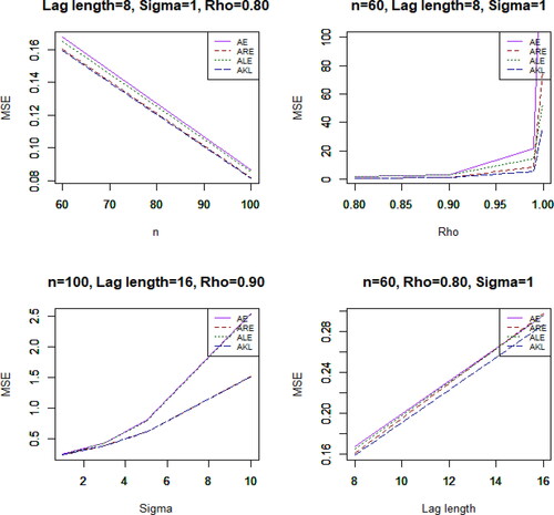
From Tables 1 and 2, we observed the following trend about the mean squared error. The mean squared error increases as the following increases: level of multicollinearity, lag length, and the error variance. The mean squared error decreases as the sample size increase. This trend is more feasible considering Figure 1. The results show that AE suffers setback when the regressors are correlated. The biased estimators provide a more consistent estimate when there is multicollinearity. However, the A-KLE produces the best result by producing smaller mean squared error among all the estimators under study.

Figure 1. Graphical illustration of the simulation result.

5. Applications

To illustrate the theoretical findings of the paper, we consider the two real datasets.

5.1. Application example I

The Almon dataset is employed to illustrate the performances of each of the estimators (Almon, 1965). These data are quarterly data that spanned from 1953 to 1967 with expenditures as the response variable and appropriations as the independent variable. Following Güler et al. (2015), the lag length is taken to be 8 and the lag weight approximated by a polynomial of order 2. The eigenvalues of $Z^{\prime }Z$ are computed to be 2.388929e + 13, 1.628323e + 09, 4.312742e + 07, and 4.782067e + 00, respectively. The condition index of $CI=\sqrt{\max (e_i)/\min (e_i)}$ is determined to be 2235083, which revealed the presence of severe multicollinearity among the explanatory variable and its lagged variables. The library dLagM in RStudio is used to analyse the data. The biasing parameter for A-RE and A-KLE is computed using: (5.1) $$\widehat{k}=\frac{(s+1){\widehat{\sigma }}^2}{\sum _{i=1}^{s+1}{\widehat{\alpha }}_i^2}.$$(5.1)

The biasing parameter for the A-LE is obtained using the following: (5.2) $$\widehat{d}=\min \left(\frac{{\widehat{\sigma }}^2}{{\widehat{\alpha }}_i^2+\frac{{\widehat{\sigma }}^2}{e_i}}\right).$$(5.2)

The regression parameter before transformation is presented in Table 3 as follows:

By canonical transformation, the $4\times 4$ matrix $\tilde{Q}$ is the matrix of the eigenvectors, $E$ is a $4\times 4$ diagonal matrix of eigenvalues of $Z^{\prime }Z$ such that $Z^{\prime }Z=QE{Q}^{\prime }.$ The Almon-estimators of $\alpha$ are presented in Table 4. The result in Table 4 supports the fact that the Almon-estimator suffers set back when there is multicollinearity. The regression coefficient of the biased estimators appears very similar. The A-KLEr has the lowest mean squared error followed by the A-RE.

Table 3. Estimates and t-tests for beta coefficients.

Coeff.	Estimate	Std. Error	t value	P(>|t|)
${\beta }_0$	0.0962	0.0168	5.71	9.04E − 07
${\beta }_1$	0.123	0.0067	18.4	3.02E − 22
${\beta }_2$	0.14	0.00552	25.3	7.47E − 28
${\beta }_3$	0.146	0.00906	16.1	4.83E − 20
${\beta }_4$	0.142	0.0103	13.7	1.80E − 17
${\beta }_5$	0.127	0.00876	14.5	2.29E − 18
${\beta }_6$	0.102	0.00541	18.9	9.77E − 23
${\beta }_7$	0.0669	0.00817	8.19	2.15E − 10
${\beta }_8$	0.0214	0.0189	1.13	2.64E − 01

Table 4. Estimates for the Almon coefficients.

Coeff.	${\widehat{\alpha }}_A$	${\widehat{\alpha }}^k$	${\widehat{\alpha }}^d$	${\widehat{\alpha }}^{KL}$
${\tilde{\alpha }}_0$	73.1	1.02E − 05	1.02E − 05	1.02E − 05
${\tilde{\alpha }}_1$	0.0962	1.05E − 01	1.05E − 01	1.05E − 01
${\tilde{\alpha }}_2$	0.0320	0.02607	0.02605	0.02608
${\tilde{\alpha }}_3$	−0.0052	−4.396E − 03	−4.394E − 03	−4.397E − 03
MSE	3397.92	194.34	232.54	145.33

Table 5. Estimates and t-tests for beta coefficients.

Coeff.	Estimate	Std. Error	t value	P(>|t|)
${\beta }_0$	1.6	1.01	1.58	0.114
${\beta }_1$	0.521	0.569	0.915	0.36
${\beta }_2$	−0.491	0.67	−0.733	0.464
${\beta }_3$	−1.43	0.569	−2.52	0.0119
${\beta }_4$	−2.31	1.01	−2.28	0.0229

5.2. Application example II

This dataset is composed of monthly global mean sea level (GMSL) (compared to 1993–2008 average) series by CSIRO, land ocean temperature anomalies (1951–1980 as a baseline period) by GISS, NASA, and monthly Southern Oscillation Index (SOI) by Australian Government Bureau of Meteorology (BOM) between July 1885 and June 2013 (Church & White, 2011; Demirhan, 2020). In this study, the response and the explanatory variables were chosen to be GMSL and land ocean temperature anomalies, respectively. The dataset is available in the R package data (seaLevelTempSOI). More detail on the data description is available in the study of Demirhan (2020). The lag length is taken to be 4 and the lag weight approximated by a polynomial of order 2 (Demirhan, 2020). The eigenvalues of $Z^{\prime }Z$ are computed to be 6607.86, 1590.99, 67.12 and 6.96, respectively. The condition number is 948.82 which shows that the explanatory variable and its lagged variables are correlated. The regression parameter before canonical transformation is presented in Table 5.

By canonical transformation, the Almon-estimators of $\alpha$ are in Table 6. From Table 6, the Almon-estimator for the second lag has a positive sign as opposed a negative sign by other estimators. As mentioned earlier, one of the effects of multicollinearity on the AE is that the coefficients can occasionally exhibit a wrong sign. The results show that the new estimator has the lowest mean squared error. This result agrees with the theoretical and simulation result.

Table 6. Estimates for the Almon coefficients.

Coeff.	${\widehat{\alpha }}_A$	${\widehat{\alpha }}^k$	${\widehat{\alpha }}^d$	${\widehat{\alpha }}^{KL}$
Intercept	0.0134	0.0133	0.0134	0.0133
${\tilde{\alpha }}_0$	1.6010	0.6354	1.4540	0.5567
${\tilde{\alpha }}_1$	−1.1149	−0.1201	−0.9409	−0.0412
${\tilde{\alpha }}_2$	0.0345	−0.1782	−0.0044	−0.1949
MSE	2.6410	0.3690	2.0740	0.3146

6. Some concluding remarks

The DLM is often adopted to predict the current values of a response variable based on both the current values of a regressor and its lagged values. Multicollinearity arises from the relationship between the regressors and their lagged explanators. The AE is popularly used to estimate the parameters of the models. However, the estimator suffers a setback when there is multicollinearity. The A-RE and A-LE estimators were suggested as alternative techniques. In this study, we developed the A-KLE to mitigate the threat of multicollinearity for the DLM. We theoretically proved that A-KLE dominates AE, A-RE and A-LE. The theoretical findings were supported by the results of the simulation study and two numerical examples.

Acknowledgements

This paper was written and completed while the first author visited Professor B. M. Golam Kibria at Florida International University from April 1 to 30, 2021. The International Mathematical Union sponsored this trip.

Disclosure statement

No potential conflict of interest was reported by the authors.

References

- Almon, S. (1965). The distributed lag between capital appropriations and expenditures. Econometrica, 30, 96–178.
- Baye, M. R., & Parker, F. D. (1984). Combining ridge and principal component regression: A money demand illustration. Communications in Statistics - Theory and Methods, 13(2), 197–205. doi:https://doi.org/10.1080/03610928408828675
- Chanda, A. K., & Maddala, G. S. (1984). Ridge estimators for distributed lag models. Communications in Statistics-Theory and Methods, 13(2), 217–225.
- Church, J. A., & White, N. J. (2011). Sea-level rise from the late 19th to the early 21st century. Surveys in Geophysics, 32(4–5), 585–602. doi:https://doi.org/10.1007/s10712-011-9119-1
- Cromwell, J. B., Hannan, M. J., Labys, W. C., & Terraza, M. (1994). Multivariate tests for time series models. Thousand Oaks, CA: Sage.
- Davidson, R., & MacKinnon, J. G. (1993). Estimation and inference in econometrics. Oxford: Oxford University Press.
- Demirhan, H. (2020). dLagM: An R package for distributed lag models and ARDL bounds testing. PLoS One, 15(2), e0228812. doi:https://doi.org/10.1371/journal.pone.0228812
- Fair, C. R., & Jaffee, M. D. (1971). A note on the estimation of polynomial distributed lags (Econometric Research Program Research Memorandum No. 120). Berkeley: University of California, Berkeley School of Law.
- Fisher, I. (1937). Income in theory and income taxation practice. Econometrica, 5(1), 1–55. doi:https://doi.org/10.2307/1905400
- Frost, P. A. (1975). Some properties of the Almon lag technique when one searches for degree of polynomial and lag. Journal of the American Statistical Association, 70(351), 606–612. doi:https://doi.org/10.2307/2285941
- Güler, H., Gültay, B., & Kaçiranlar, S. (2015). Comparisons of the alternative biased estimators for the distributed lag models. Communications in Statistics - Simulation and Computation. doi:https://doi.org/10.1080/03610918.2015.1053919
- Gültay, B., & Kaçıranlar, S. (2015). Mean square error comparisons of the alternative estimators for the distributed lag models. Hacettepe Journal of Mathematics and Statistics, 44(5), 1215–1233.
- Hoerl, A. E., & Kennard, R. W. (1970). Ridge regression: Biased estimation for non orthogonal problems. Technometrics, 12(1), 69–82. doi:https://doi.org/10.1080/00401706.1970.10488635
- Judge, G. G., Griffiths, W. E., Hill, R. C., & Lee, T. (1980). The theory and practice of econometrics. New York, NY: Wiley (pp. 637–660).
- Kaçıranlar, S., & Sakallıoğlu, S. (2001). Combining the Liu estimator and the principal component regression estimator. Communications in Statistics - Theory and Methods, 30(12), 2699–2705. doi:https://doi.org/10.1081/STA-100108454
- Kibria, G. B. M., & Lukman, A. F. (2020). A new ridge-type estimator for the linear regression model: Simulations and applications. Scientifica, 2020, 1–16. doi:https://doi.org/10.1155/2020/9758378
- Li, Y., & Yang, H. (2012). A new Liu-type estimator in linear regression model. Statistical Papers, 53(2), 427–437. doi:https://doi.org/10.1007/s00362-010-0349-y
- Lindley, D. V., & Smith, A. F. M. (1972). Bayes estimates for the linear model. Journal of the Royal Statistical Society: Series B (Methodological), 34(1), 1–41. doi:https://doi.org/10.1111/j.2517-6161.1972.tb00885.x
- Lipovetsky, S. (2006). Two parameter ridge regression and its convergence to the eventual pairwise model. Mathematical and Computer Modeling, 44(3–4), 304–318. doi:https://doi.org/10.1016/j.mcm.2006.01.017
- Lipovetsky, S., & Conklin, W. M. (2005). Ridge regression in two parameter solution. Applied Stochastic Models in Business and Industry, 21(6), 525–540. doi:https://doi.org/10.1002/asmb.603
- Liu, K. (1993). A new class of biased estimate in linear regression. Communication in Statistics-Theory and Methods, 22(2), 393–402.
- Lukman, A. F., Ayinde, K., Binuomote, S., & Onate, A. C. (2019). Modified ridge‐type estimator to combat multicollinearity: Application to chemical data. Journal of Chemometrics, 33(5), e3125. doi:https://doi.org/10.1002/cem.3125
- Lukman, A. F., Ayinde, K., Kibria, G. B. M., & Adewuyi, E. (2020). Modified ridge-type estimator for the gamma regression model. Communications in Statistics - Simulation and Computation, 1–15. doi:https://doi.org/10.1080/03610918.2020.1752720
- Maddala, G. S. (1974). Ridge estimator for distributed lag models (NBER Working Paper Series No. 69). Cambridge, MA: National Bureau of Economic Research.
- Majid, A., Aslam, M., Altaf, S., & Amanullah, M. (2019). Addressing the distributed lag models with heteroscedastic errors. Communications in Statistics - Simulation and Computation, 1–19. doi:https://doi.org/10.1080/03610918.2019.1643884
- Massy, W. F. (1965). Principal component regression in explanatory statistical research. Journal of the American Statistical Association, 60(309), 234–256. doi:https://doi.org/10.1080/01621459.1965.10480787
- Ozbay, N. (2019). Two-parameter ridge estimation for the coefficients of Almon distributed lag model. Iranian Journal of Science and Technology, Transactions A: Science, 43 (4), 1819–1828.
- Özbay, N., & Kaçıranlar, S. (2017). The Almon two parameter estimator for the distributed lag models. Journal of Statistical Computation and Simulation, 87(4), 834–843. doi:https://doi.org/10.1080/00949655.2016.1229317
- Özbay, N., & Toker, S. (2021). Prediction framework in a distributed lag model with a target function: An application to global warming data. Environmental and Ecological Statistics, 28(1), 87–134. doi:https://doi.org/10.1007/s10651-020-00477-x
- Özkale, M. R., & Kaçıranlar, S. (2007). The restricted and unrestricted two parameter estimators. Communications in Statistics - Theory and Methods, 36(15), 2707–2725. doi:https://doi.org/10.1080/03610920701386877
- R Core Team. (2020). R: A language and environment for statistical computing. Vienna, Austria: R Foundation for Statistical Computing. Retrieved from https://www.R-project.org.
- Swindel, B. (1976). Good ridge estimators based on prior information. Communication in Statistics-Theory and Methods, A5, 1065–1075.
- Trenkler, G., & Toutenburg, H. (1990). Mean squared error matrix comparisons between biased estimators—An overview of recent results. Statistical Papers, 31(1), 165–179. doi:https://doi.org/10.1007/BF02924687
- Vinod, H. D., & Ullah, A. (1981). Recent advances in regression methods. New York, NY: Marcel Dekker (pp. 226–238).
- Yeo, S. J., & Trivedi, P. K. (2009). On using ridge-type estimators for a distributed lag model. Oxford Bulletin of Economics and Statistics, 51(1), 85–90. doi:https://doi.org/10.1111/j.1468-0084.1989.mp51001006.x