Time-fractional partial differential equations: a novel technique for analytical and numerical solutions

Abstract

We use the q-homotopy analysis Shehu transform method in this article to obtain analytical and numerical solutions to time fractional partial differential equations. We also give analytical solutions to two problems, as well as a comparison study in terms of absolute error with homotopy perturbation transform method, homotopy analysis transform method, and residual power series method to verify the suggested technique’s effectiveness and correctness. The numerical and graphical solutions achieved by the proposed method show that it is computationally accurate and may be used to obtain and investigate solutions to time fractional partial differential equations.

Keywords:

• The q-homotopy analysis method
• fractional differential equation
• proportional delay
• Shehu transform
• Caputo approach

1. Introduction

Fractional calculus (FC), including integration and differentiation of arbitrary non-integer order, is the generalization of classical integration and differentiation (Oldham & Spanier, 1974). The beauty of FC is that fractional order derivatives and integrals are non-local. The purpose of using fractional models in differential equations in physical models (Ali, Osman, Baskonus, Elazabb, & İlhan, 2020; Cuahutenango-Barro et al., 2021; Khalid, Rehan, Nisar, & Osman, 2021) due to their non-local property. Recently, numerous models in biology (Dave, Khan, Purohit, & Suthar, 2021; Kumar, Kumar, Osman, & Samet, 2021; Mistry, Khan, & Suthar, 2020; Nisar et al., 2022), and dynamics (Bayones et al., 2021) can be modelled with the help of fractional order derivatives. In the past few years, many researchers have been established and applied numerous schemes to gain the solutions of fractional order differential equations such as (Akinyemi, Şenol, & Osman, 2022; Ramani et al., 2022, Ramani, Khan, & Suthar, 2019), HATM and RPSM (Wang, Wu, Ren, & Chen, 2019), reproducing kernel discretization method (Arqub, Osman, Abdel-Aty, Mohamed, & Momani, 2020), Chebyshev wavelet collocation method (Dhawan, Machado, Brzeziński, & Osman, 2021), Chebyshev collocation method (Ali, Abd El Salam, et al., 2020; Habenom & Suthar, 2020), Tikhonov regularization method (Djennadi, Shawagfeh, & Abu Arqub, 2021; Djennadi, Shawagfeh, Osman, Gómez-Aguilar, & Arqub, 2021), the Adams-Bashforth predictor-corrector method (Kumar, Chauhan, Osman, & Mohiuddine, 2021), Haar wavelet method (Amin, Mahariq, Shah, Awais, & Elsayed, 2021), reproducing kernel method (AL-Smadi, Arqub, & El-Ajou, 2014; Yildirim, Akgül, & Inc, 2021), Homotopy perturbation method (He, 1999; Pareek, Gupta, Agarwal, & Suthar, 2021).

In the present paper, we consider the initial value autonomous system of time fractional partial differential equations (TFPDEs) with proportional delay defined in (Sakar, Uludag, & Erdogan, 2016) (1) $$\{\begin{array}{c}{}^C{D}_{\tau }^{\zeta }\nu \left(\eta ,\tau \right)=\varphi \left(\eta ,\nu \left(a_0\eta ,b_0\tau \right),\frac{\partial }{\partial \eta }\nu \left(a_1\eta ,b_1\tau \right),\dots ,\frac{{\partial }^p}{\partial {\eta }^p}\nu \left(a_p\eta ,b_p\tau \right)\right),\hfill \\ {\nu }^i\left(\eta ,0\right)= h_i\left(\eta \right). \hfill \end{array}$$(1) where $a_j, b_j\in (0,1)$ with $j=\{0, 1, 2,\dots ,p\},h_i(\eta )$ represents the initial value, and $\varphi$ denotes the differential operator. $D_{\tau }^{\zeta }\nu (\eta ,\tau )$ presents the Caputo derivative of $\nu (\eta ,\tau ).$

El-Tawil and Huseen (2012, 2013) proposed a method namely q-homotopy analysis method (q-HAM) which is a more general method of HAM. The essential idea of this method is to introduce a homotopy parameter, say q, which varies from 0 to $1/n, n\ge 1$ and a nonzero auxiliary parameter $\hslash .$ At q = 0, the system of equations usually has been reduced to a simplified form which normally admits a rather simple solution. As q gradually increases continuously towards $1/n,$ the system goes through a sequence of deformations, and the solution at each stage is close to that at the previous stage of the deformation. Eventually at $q=1/n,$ the system takes the original form of the equation and the final stage of the deformation gives the desired solution.

The Shehu transform (ST) is a generalization of the Laplace and the Sumudu integral transform (Watugala, 1998). Besides, the proposed integral transform is similar to natural transform (Khan & Khan, 2008). The ST become Laplace’s transform (Spiegel, 1965), when the variable μ = 1, and becomes the Yang’s integral transform (Yang, 2016) when the variable s = 1.

In this study, we used q-homotopy analysis Shehu transform method (q-HASTM) to gain the analytical solution of system (1). The proposed scheme, namely q-HASTM, is an elegant amalgamation of q-HAM and ST. Its superiority is its ability to adjust two strong computational methodologies for probing FDEs. By choosing proper $\hslash ,$ we can control the convergence region of solution series in a large permissible domain. The advantage of q-HASTM in that it does not require linearization or discretization, shows little perturbations, has no restrictive assumptions, lessens mathematical computations significantly, offers non-local effect, promises a big convergence region and is free from obtaining difficult polynomials, integrations and physical parameters.

2. Definitions

Definition 2.1.

The fractional Caputo derivative of function $\nu \in C_{-1}^m$ is defined as (Diethelm & Ford, 2002) (2) $${}^C{D}_{\tau }^{\zeta }\nu \left(\eta ,\tau \right)=\{\begin{array}{c}\frac{{\partial }^m\nu \left(\eta ,\tau \right)}{\partial {\eta }^m}, \zeta =m\in \aleph ,\hfill \\ \frac{1}{\Gamma \left(m-1\right)}\underset{0}{\overset{\tau }{\int }}{\left(\tau -\upsilon \right)}^{m-1-\zeta }\frac{{\partial }^m\nu \left(\eta ,\upsilon \right)}{\partial {\upsilon }^m}d\upsilon , m-1<\zeta \le 1. \hfill \end{array}$$(2)

In particular, if $0<\zeta <1,,$ then ${}^C{D}_{\tau }^{\zeta }\nu (\eta ,\tau )=\frac{1}{\Gamma (1-\zeta )}{\int }_0^{\tau }{(\tau -\xi )}^{-\zeta }\frac{\partial \nu (\eta ,\xi )}{\partial \xi }d\xi .$

Lemma 2.1.

The Caputo derivative ${}^C{D}_{\tau }^{\zeta }$ satisfies some following properties for $0<\zeta \le 1, \phi >-1.$

1. ${}^C{D}_{\tau }^{\zeta }$p = 0, for a constant;

2. $J_{\tau }^{\zeta }{D}_{\tau }^{\zeta }\nu (\eta ,\tau )=\nu (\eta ,\tau )-\nu (\eta ,0);$

3. ${}^C{D}_{\tau }^{\zeta } {\tau }^{\phi }= \frac{\Gamma (1+\phi )}{\Gamma (1+\phi -\zeta )}{\tau }^{\varphi -\zeta }.$

Definition 2.2.

The ST (Maitama & Zhao, 2019b) of the function $\nu (\tau )$ of exponential order is defined over the set of functions, $$A=\{\nu \left(\tau \right) : \exists F, {\gamma }_1, {\gamma }_2 >0, |\nu \left(\tau \right)|< F\text{exp}\hspace{0.17em}(\frac{\left|\tau \right|}{{\gamma }_i}), if \tau \in {(-1)}^i\times [0,\infty )\},$$ by the following integral (3) $$S\left[\nu \left(\tau \right)\right]= V\left(s,\mu \right)=\underset{0}{\overset{\infty }{\int }}\hspace{0.17em}\text{exp}\hspace{0.17em}\left(-\frac{s\tau }{\mu }\right)\nu \left(\tau \right) d\tau , s>0, \mu >0.$$(3)

It converges if the limit of the integral exists, and diverges if not.

Definition 2.3.

The ST of Caputo fractional derivative operator was introduced by Maitama and Zhao (2019b) and expressed as (4) $$S\left[{}^C{D}_{\tau }^{\zeta }\nu \left(\eta ,\tau \right)\right] = {\left(\frac{s}{\mu }\right)}^{\zeta }\vartheta \left(s,\mu \right)-\sum _{r=0}^{m-1}{\left(\frac{s}{\mu }\right)}^{\zeta -r-1}{\nu }^{\left(r\right)}\left(o^{+}\right),$$(4) here $\vartheta (s,\mu )$ is the ST of $\nu (\tau ).$

3. Basic idea of proposed technique

Consider a time fractional partial differential system (5) $$\{\begin{array}{c}{D}_{\tau }^{\zeta }\nu \left(\eta ,\tau \right)=\varphi \left(\eta ,\nu \left(a_0\eta ,b_0\tau \right),\frac{\partial }{\partial \eta }\nu \left(a_1\eta ,b_1\tau \right),\dots ,\frac{{\partial }^p}{\partial {\eta }^p}\nu \left(a_p\eta ,b_p\tau \right)\right),\hfill \\ \nu \left(\eta ,0\right)= h\left(\eta \right). \hfill \end{array}$$(5) where $0 <\zeta \le 1,D_{\tau }^{\zeta }\nu (\eta ,\tau )$ presents the Caputo derivative of $\nu (\eta ,\tau )$ and $\varphi$ denotes the differential operator.

Taking the ST to both sides of Equation (5) and on simplifying, we get (6) $$\begin{array}{c}S[\nu (\eta ,\tau )]-\frac{\mu }{s}\nu (\eta ,0)-{(\frac{\mu }{s})}^{\zeta }S[\varphi (\eta ,\nu (a_0\eta ,b_0\tau ),\frac{\partial }{\partial \eta }\nu (a_1\eta ,b_1\tau ),\dots ,\frac{{\partial }^p}{\partial {\eta }^p}\nu (a_p\eta ,b_p\tau ))]=0 .\hfill \end{array}$$(6)

Now, we define a non-linear operator as (7) $$\begin{array}{c}N[\Upsilon (\eta ,\tau ;q)]=S[\Upsilon (\eta ,\tau ;q)]-\frac{\mu }{s}(\nu (\eta ,0))\hfill \\ -{(\frac{\mu }{s})}^{\zeta }S[\varphi (\eta ,{\rm Y}(a_0\eta ,b_0\tau ;q),\frac{\partial }{\partial \eta }\Upsilon (a_1\eta ,b_1\tau ;q),\dots ,\frac{{\partial }^p}{\partial {\eta }^p}\Upsilon (a_p\eta ,b_p\tau ;q))].\hfill \end{array}$$(7)

In Equation (7), $q\in \left[0,\frac{1}{n}\right]$ is an embedding parameter and $\Upsilon (\eta ,\tau ;q)$ is indicate the real function of $\eta ,\tau$ and q. Liao (1992, 1995) constructed zeroth-order deformation equation such as (8) $$\left(1-nq\right)S\left[\Upsilon \left(\eta ,\tau ;q\right)-\nu \left(\eta ,0\right)\right]=\hslash H\left(\eta ,\tau \right)qN\left[\Upsilon \left(\eta ,\tau ;q\right)\right],$$(8) here S represents the ST, $\hslash$ is nonzero auxiliary parameter, $H(\eta ,\tau )\ne 0$ denoted an auxiliary function, and $\nu (\eta ,0)$ expresses the initial gauss of $\nu (\eta ,\tau ),$ and $\Upsilon (\eta ,\tau ;q)$ is unknown function. Let q = 0 and q = 1 in Equation (8), we get (9) $$\Upsilon \left(\eta ,\tau ;0\right)={\nu }_0\left(\eta ,\tau \right), \Upsilon \left(\eta ,\tau ;\frac{1}{n}\right)=\nu \left(\eta ,\tau \right).$$(9)

Thus, if q rises from 0 to $\frac{1}{n},$ the series solution $\Upsilon (\eta ,\tau ;q)$ varies from the initial guess ${\nu }_0(\eta ,\tau )$ to the solution $\nu (\eta ,\tau ).$ Upon expanding $\Upsilon (\eta ,\tau ;q)$ with the help of Taylor’s series near to q, we have (10) $$\Upsilon \left(\eta ,\tau ;q\right)={\nu }_0\left(\eta ,\tau \right)+\sum _{p=1}^{\infty }{\nu }_p\left(\eta ,\tau \right)q^p,$$(10) where (11) $${\nu }_p\left(\eta ,\tau \right)=\frac{1}{p!}{\frac{{\partial }^p\Upsilon \left(\eta ,\tau ;q\right)}{\partial q^p}|}_{q=0} .$$(11)

By proper choosing of ${\nu }_0(\eta ,\tau ),\hslash ,$ and $H(\eta ,\tau )$ the series in Equation (10) converges at q = $\frac{1}{n},$ we will get (12) $$\nu (\eta ,\tau ) = {\nu }_0\left(\eta ,\tau \right)+\sum _{p=1}^{\infty }{\nu }_p\left(\eta ,\tau \right){\left(\frac{1}{n}\right)}^p.$$(12)

We define the vector $\overrightarrow{{\nu }_p}(\eta ,\tau )$ as (13) $$\overrightarrow{{\nu }_p}(\eta ,\tau ) = \left\{{\nu }_0(\eta ,\tau ), {\nu }_1(\eta ,\tau ),\dots , {\nu }_p(\eta ,\tau )\right\}.$$(13)

First, differentiating Equation (8) p-times with respect to q, then evaluate at q = 0 and finally dividing by $\Gamma (p+1),$ we have the so-called pth-order deformation equation (14) $$S\left[{\nu }_p\left(\eta ,\tau \right)-{\chi }_p{\nu }_{p-1}\left(\eta ,\tau \right)\right] = \hslash H\left(\eta ,\tau \right){\mathfrak{R}}_p\left[{\overrightarrow{\nu }}_{p-1}\left(\eta ,\tau \right)\right].$$(14) where (15) $${\mathfrak{R}}_p\left[{\overrightarrow{\nu }}_{p-1}\left(\eta ,\tau \right)\right] = \frac{1}{\left(p-1\right)!}{\frac{{\partial }^{p-1}\left[N\Upsilon \left(\eta ,\tau ;q\right)\right]}{\partial q^{p-1}}|}_{q=0} ,$$(15) and (16) $${\chi }_p = \{\begin{array}{c}0, p\le 1\hfill \\ n, \text{otherwise} .\hfill \end{array}$$(16)

Taking the inverse ST to both sides of Equation (14) and with the aid of Equations (8) and (15), we get (17) $${\nu }_p\left(\eta ,\tau \right)={\chi }_p{\nu }_{p-1}\left(\eta ,\tau \right)+S^{-1}\left[\hslash H\left(\eta ,\tau \right){\mathfrak{R}}_p\left[{\overrightarrow{\nu }}_{p-1}\left(\eta ,\tau \right)\right]\right].$$(17)

Based on Equation (5), ${\mathfrak{R}}_p\left[{\overrightarrow{\nu }}_{p-1}(\eta ,\tau )\right]$ is define as (18) $$\begin{array}{c}{\mathfrak{R}}_p[{\overrightarrow{\nu }}_{p-1}(\eta ,\tau )]=S[{\nu }_{p-1}(\eta ,\tau )]-\frac{\mu }{s}{\nu }_0(\eta ,\tau )(1-\frac{{\chi }_p}{n})-{(\frac{\mu }{s})}^{\zeta }S[\varphi (\eta , {\nu }_{p-1}(a_0\eta ,b_0\tau ),\frac{\partial ({\nu }_{p-1}(a_1\eta ,b_1\tau ))}{\partial \eta },\dots , \frac{{\partial }^p({\nu }_{p-1}(a_p\eta ,b_p\tau ))}{\partial {\eta }^p})],\hfill \end{array}$$(18)

Finally, we compute ${\nu }_p(\eta ,\tau )$ by using Equation (17) for $p\ge 1.$ Hence the Mth order approximate solution of Equation (5) can be represented as (19) $$\nu \left(\eta ,\tau \right)=\sum _{p=0}^M{\nu }_p\left(\eta ,\tau \right){\left(\frac{1}{n}\right)}^p ,$$(19)

Moreover, for $M\to \infty ,$ we get (20) $$\nu \left(\eta ,\tau \right)=\sum _{p=0}^{\infty }{\nu }_p\left(\eta ,\tau \right){\left(\frac{1}{n}\right)}^p .$$(20)

The existence of the factor ${(\frac{1}{n})}^p$ in the q-HASTM solution (20) allows for faster convergence than the standard HAM. Moreover, in the special case n = 1, the q-HASTM reduces to the standard homotopy analysis Shehu transform method (HASTM).

4. Convergence analysis

In this section, we investigate the convergence analysis of q-HASTM technique.

Theorem 4.1.

Let $\mathfrak{R}(\nu )$ satisfy the Lipschitz condition with the Lipschitz constant δ. The solution derived with the aid of q-HASTM of the time fractional partial differential system (5) is unique, wherever $0<\sigma <1$, where $\sigma =(n+\hslash ) + \hslash \delta T.$

Proof.

The solution of the time fractional partial differential system (5) is presented as (21) $$\nu \left(\eta ,\tau \right)=\sum _{p=0}^{\infty }{\nu }_p\left(\eta ,\tau \right){\left(\frac{1}{n}\right)}^p,$$(21) where (22) $$\begin{array}{c}{\nu }_p(\eta , \tau )=({\chi }_p+\hslash ){\nu }_{p-1}(\eta , \tau )-(1-\frac{{\chi }_p}{n})S^{-1}((\frac{\mu }{s}){\nu }_0(\eta , \tau ))-\hslash S^{-1}[{(\frac{\mu }{s})}^{\zeta }S[\varphi (\eta ,{\nu }_{p-1}(a_0\eta , b_0\tau ),\frac{\partial }{\partial \eta }({\nu }_{p-1}(a_1\eta , b_1\tau )),\dots ,\frac{{\partial }^p}{\partial {\eta }^p}({\nu }_{p-1}(a_p\eta , b_p\tau )))]].\hfill \end{array}$$(22)

Now, let ν and ${\nu }^{*}$ be two different solutions of considered time fractional partial differential system, then we have (23) $$|\nu - {\nu }^{*}|=|(n+\hslash )(\nu - {\nu }^{*})+\hslash S^{-1}[{(\frac{\mu }{s})}^{\zeta }S(\mathfrak{R}(\nu - {\nu }^{*}))]|.$$(23)

With the aid of the convolution theorem, we can obtain (24) $$\begin{array}{l}|\nu - {\nu }^{*}|\le (n+\hslash )|\nu - {\nu }^{*}|+\hslash \underset{0}{\overset{\tau }{\int }}(|\mathfrak{R}(\nu - {\nu }^{*})|)\frac{{(\tau -\xi )}^{\zeta }}{\Gamma (\zeta +1)}d\zeta ,\le (n+\hslash )|\nu - {\nu }^{*}|+\hslash \underset{0}{\overset{\tau }{\int }}(\delta |(\nu - {\nu }^{*})|)\frac{{(\tau -\xi )}^{\zeta }}{\Gamma (\zeta +1)}d\zeta . \hfill \end{array}$$(24)

Next, putting up the integral mean value theorem in use, it yields (25) $$\begin{array}{c}|\nu - {\nu }^{*}|\le \left(n+\hslash \right)\left|\nu - {\nu }^{*}\right|+\hslash \left(\delta \left|\left(\nu - {\nu }^{*}\right)\right|\right)T,\hfill \\ \le \left|\nu - {\nu }^{*}\right|\sigma . \hfill \end{array}$$(25)

It gives $(1-\sigma )|\nu - {\nu }^{*}|\le 0 .$ Because $0<\sigma <1;$ therefore, $\left|\nu - {\nu }^{*}\right|=0,$ which implies that $\nu = {\nu }^{*}.$ Hence the solution is unique.

Theorem 4.2

(Convergence theorem). Let us consider that X be a Banach space and there is a nonlinear mapping $B: X\to X$ and assume that (26) $$\Vert W\left(\nu \right)-W\left(r\right)\Vert \le \sigma \Vert \nu -r\Vert , \forall \nu ,r\in X.$$(26)

Then in view of Banach’s fixed point theory, W has a fixed point. Furthermore, the sequence generated by the q-HASTM with an arbitrary selection of ${\nu }_0, r_0\in X$ converges to the fixed point of W and (27) $$\Vert {\nu }_m-{\nu }_n\Vert \le \frac{{\sigma }^n}{1-\sigma }\Vert {\nu }_1-{\nu }_0\Vert , \forall \nu ,r\in X.$$(27)

Proof.

Let us take a Banach space $(C\left[I\right], \Vert .\Vert )$ of all continuous functions on I with the norm expressed as $\Vert g(\tau )\Vert =\underset{\tau \in I}{\max }\left|g(\tau )\right| .$

Now, we show that the sequence $\left\{{\nu }_n\right\}$ is a Cauchy sequence in the Banach space. $$\begin{array}{c}\Vert {\nu }_m-{\nu }_n\Vert = \underset{\tau \in I}{\max }|{\nu }_m-{\nu }_n| \hfill \\ \underset{\tau \in I}{\max }|(n+\hslash )({\nu }_{m-1}-{\nu }_{n-1})+\hslash S^{-1}({(\frac{\mu }{s})}^{\zeta }S(\mathfrak{R}({\nu }_{m-1}- {\nu }_{n-1})))| \hfill \\ \le \underset{\tau \in I}{\max }(n+\hslash )|{\nu }_{m-1}-{\nu }_{n-1}| +\hslash S^{-1} ({(\frac{\mu }{s})}^{\zeta }S(\mathfrak{R}|{\nu }_{m-1}- {\nu }_{n-1}|)) .\hfill \end{array}$$

Now, making use of the convolution theorem for the ST, it gives (28) $$\begin{array}{c} \Vert {\nu }_m-{\nu }_n\Vert \le \underset{\tau \in I}{\max }[(n+\hslash )|{\nu }_{m-1}-{\nu }_{n-1}| +\hslash \underset{0}{\overset{\tau }{\int }}(|\mathfrak{R}({\nu }_{m-1}- {\nu }_{n-1})|)\frac{{(\tau -\xi )}^{\zeta }}{\Gamma (\zeta +1)}d\zeta ] \hfill \\ \le \underset{\tau \in I}{\max }[(n+\hslash )|{\nu }_{m-1}-{\nu }_{n-1}| +\hslash \underset{0}{\overset{\tau }{\int }}(\delta |({\nu }_{m-1}- {\nu }_{n-1})|)\frac{{(\tau -\xi )}^{\zeta }}{\Gamma (\zeta +1)}d\zeta ].\hfill \end{array}$$(28)

Next, by the application of the integral mean value theorem (Maitama & Zhao, 2019a), we obtain $$\begin{array}{c}\Vert {\nu }_m-{\nu }_n\Vert \le \underset{\tau \in I}{\max }[(n+\hslash )|{\nu }_{m-1}- {\nu }_{n-1}|+\hslash (\delta |({\nu }_{m-1}- {\nu }_{n-1})|)T]\hfill \\ \le \sigma \Vert {\nu }_{m-1}-{\nu }_{n-1}\Vert .\hfill \end{array}$$

Let m = n + 1, then we have (29) $$\Vert {\nu }_{n+1}-{\nu }_n\Vert \le \sigma \Vert {\nu }_n-{\nu }_{n-1}\Vert \le {\sigma }^2\Vert {\nu }_{n-1}-{\nu }_{n-2}\Vert \le \cdots \le {\sigma }^n\Vert {\nu }_1-{\nu }_0\Vert .$$(29)

On using the triangular inequality, it yields $$\begin{array}{c}\Vert {\nu }_m-{\nu }_n\Vert \le \Vert {\nu }_{n+1}-{\nu }_n\Vert +\Vert {\nu }_{n+2}-{\nu }_{n+1}\Vert +\cdots +\Vert {\nu }_m-{\nu }_{m-1}\Vert \hfill \\ \le \left[{\sigma }^n+{\sigma }^{n+1}+\cdots +{\sigma }^{m-1}\right]\Vert {\nu }_1-{\nu }_0\Vert \hfill \\ \le {\sigma }^n\left[1+\sigma +{\sigma }^2+\cdots +{\sigma }^{m-n-1}\right]\Vert {\nu }_1-{\nu }_0\Vert \hfill \\ \le {\sigma }^n\left[\frac{1-{\sigma }^{m-n-1}}{1-\sigma }\right]\Vert {\nu }_1-{\nu }_0\Vert .\hfill \end{array}$$

Because $0<\sigma <1,$ so $1-{\sigma }^{m-n-1}<1,$ then we have (30) $$\Vert {\nu }_m-{\nu }_n\Vert \le \frac{{\sigma }^n}{1-\sigma }\Vert {\nu }_1-{\nu }_0\Vert .$$(30)

But $\Vert {\nu }_1-{\nu }_0\Vert <\infty ,$ so as $m\to \infty$ then $\Vert {\nu }_m-{\nu }_n\Vert \to 0.$ Therefore, the sequence $\left\{{\nu }_n\right\}$ is Cauchy sequence in $C\left[I\right],$ and so the sequence is convergent.

5. Numerical problem

In this section, we consider two numerical problems to prove the accuracy, and efficiency of our proposed method. All the numerical and graphical results for the following two problems are calculated by utilizing the software scilab-6.0.2.

Problem 1.

Consider the time-fractional generalized Burger’s equation (Sakar et al., 2016) as (31) $${}^C{D}_{\tau }^{\zeta }\nu \left(\eta ,\tau \right)=\nu \left(\frac{\eta }{2},\frac{\tau }{2}\right)\frac{\partial }{\partial \eta }\nu \left(\eta ,\frac{\tau }{2}\right)+\frac{{\partial }^2}{\partial {\eta }^2}\nu \left(\eta ,\tau \right)+\frac{1}{2}\nu \left(\eta ,\tau \right),$$(31) where $0<\zeta \le 1,D_{\tau }^{\zeta }\nu (\eta ,\tau )$ presents the Caputo derivative of $\nu (\eta ,\tau )$ and subject to initial condition (32) $$\nu \left(\eta ,0\right)= \eta .$$(32)

By performing the ST on both sides of Equation (31) and with the help of Equation (32), we get (33) $$S[\nu (\eta ,\tau )]-\frac{\mu }{s}(\nu (\eta ,0))-{(\frac{\mu }{s})}^{\zeta }S[\nu (\frac{\eta }{2},\frac{\tau }{2})\frac{\partial \nu (\eta ,\frac{\tau }{2})}{\partial \eta }+\frac{{\partial }^2\nu (\eta ,\tau )}{\partial {\eta }^2}+\frac{1}{2}\nu (\eta ,\tau )]=0 .$$(33)

According to proposed scheme, we define the non-linear operator as (34) $$\begin{array}{c}N[\Upsilon (\eta ,\tau ;q)]=S[\Upsilon (\eta ,\tau ;q)]-\frac{\mu }{s}\left(\eta \right)-{(\frac{\mu }{s})}^{\zeta }S\{\Upsilon (\frac{\eta }{2},\frac{\tau }{2};q)\frac{\partial \Upsilon (\eta ,\frac{\tau }{2};q)}{\partial \eta }+\frac{{\partial }^2\Upsilon (\eta ,\tau ;q)}{\partial {\eta }^2}+\frac{1}{2}\Upsilon (\eta ,\tau ;q)\} . \hfill \end{array}$$(34)

Form Equation (14) and choosing $H(\eta ,\tau )=1,$ the pth order deformation equation is given as (35) $$\begin{array}{c}S\left[{\nu }_p\left(\eta ,\tau \right) -{\chi }_p{\nu }_{p-1}\left(\eta ,\tau \right)\right] =\hslash {\mathfrak{R}}_p\left[{\overrightarrow{\nu }}_{p-1}\right], \hfill \end{array}$$(35) and by using of Equations (15) and (34) the valve of ${\mathfrak{R}}_p\left[{\overrightarrow{\nu }}_{p-1}\right]$ is given as (36) $$\begin{array}{c}{\mathfrak{R}}_p[{\overrightarrow{\nu }}_{p-1}(\eta ,\tau )]=S[{\nu }_{p-1}(\eta ,\tau )]-(1-\frac{{\chi }_p}{n})(\frac{\mu }{s})\eta -{(\frac{\mu }{s})}^{\zeta }S[\sum _{k=0}^{p-1}\frac{\partial {\nu }_k(\eta ,\frac{\tau }{2})}{\partial \eta }{\nu }_{p-1-k}(\frac{\eta }{2},\frac{\tau }{2})\hfill \\ +\frac{{\partial }^2{\nu }_{p-1}(\eta ,\tau )}{\partial {\eta }^2}+\frac{1}{2}[{\nu }_{p-1}(\eta ,\tau )]].\hfill \end{array}$$(36)

Operating the inverse ST to Equation (35) and by using Equation (36), we get (37) $$\begin{array}{c}{\nu }_p(\eta ,\tau )= ({\chi }_p+\hslash ){\nu }_{p-1}(\eta ,\tau )-(1-\frac{{\chi }_p}{n})\hslash \eta -\hslash S^{-1}[{(\frac{\mu }{s})}^{\zeta }S[\sum _{k=0}^{p-1}\frac{\partial {\nu }_k(\eta ,\frac{\tau }{2})}{\partial \eta }{\nu }_{p-1-k}(\frac{\eta }{2},\frac{\tau }{2})\hfill \\ +\frac{{\partial }^2{\nu }_{p-1}(\eta ,\tau )}{\partial {\eta }^2}+\frac{1}{2}[{\nu }_{p-1}(\eta ,\tau )]]].\hfill \end{array}$$(37)

By putting p = 1, 2, 3 in Equation (37) and with Equation (32), we obtain the following results (38) $$\begin{array}{c}{\nu }_1(\eta ,\tau )=-\hslash S^{-1}[{(\frac{\mu }{s})}^{\zeta }S[\frac{\partial {\nu }_0(\eta ,\frac{\tau }{2})}{\partial \eta }{\nu }_0(\frac{\eta }{2},\frac{\tau }{2})+\frac{{\partial }^2{\nu }_0(\eta ,\tau )}{\partial {\eta }^2}+\frac{1}{2}{\nu }_0(\eta ,\tau )]],\\ {\nu }_1(\eta ,\tau )=-\hslash \eta \frac{{\tau }^{\zeta }}{(\Gamma (\zeta +1))},\end{array}$$(38) (39) $$\begin{array}{c}\begin{array}{c}{\nu }_2(\eta ,\tau )=(n+\hslash ){\nu }_1(\eta ,\tau )-\hslash S^{-1}[{(\frac{\mu }{s})}^{\zeta }S[\frac{\partial {\nu }_0(\eta ,\frac{\tau }{2})}{\partial \eta }{\nu }_1(\frac{\eta }{2},\frac{\tau }{2})\hfill \\ +\frac{\partial {\nu }_1(\eta ,\frac{\tau }{2})}{\partial \eta }{\nu }_0(\frac{\eta }{2},\frac{\tau }{2})+\frac{{\partial }^2{\nu }_1(\eta ,\tau )}{\partial {\eta }^2}+\frac{1}{2}{\nu }_1(\eta ,\tau )]],\hfill \end{array}\\ {\nu }_2(\eta ,\tau )=-(n+\hslash )\hslash \eta \frac{{\tau }^{\zeta }}{\Gamma (\zeta +1)}+(2^{-\zeta }+2^{-1}){\hslash }^2\eta \frac{{\tau }^{2\zeta }}{\Gamma (2\zeta +1)},\end{array}$$(39)

In the same manner, we can get (40) $$\begin{array}{l}{\nu }_3(\eta ,\tau )=-{(n+\hslash )}^2\hslash \eta \frac{{\tau }^{\zeta }}{\Gamma (\zeta +1)}+(2^{1-\zeta }+1)(n+\hslash ){\hslash }^2\eta \frac{{\tau }^{2\zeta }}{\Gamma (2\zeta +1)}\hfill \\ -(2^{-3\zeta }+2^{-1-2\zeta }+2^{-1-\zeta }+4^{-1}+\frac{\Gamma (2\zeta +1)}{{(\Gamma (\zeta +1))}^2}{2}^{-1-2\zeta }){\hslash }^3\eta \frac{{\tau }^{3\zeta }}{\Gamma (3\zeta +1)},\hfill \end{array}$$(40) (41) $$\begin{array}{l}{\nu }_4(\eta ,\tau )=-{(n+\hslash )}^3\hslash \eta \frac{{\tau }^{\zeta }}{\Gamma (\zeta +1)}+(\frac{3}{2}+2^{-\zeta }+2^{1-\zeta }){(n+\hslash )}^2{\hslash }^2\eta \frac{{\tau }^{2\zeta }}{\Gamma (2\zeta +1)}-(2^{-\zeta }\\ +2^{-2\zeta }+2^{-3\zeta }+2^{-1}+2^{-1-\zeta }+2^{-1-2\zeta }+2^{1-3\zeta }+2^{-2}+(2^{-1-2\zeta }+2^{-2\zeta })\\ \times \frac{\Gamma (2\zeta +1)}{{(\Gamma (\zeta +1))}^2})(n+\hslash ){\hslash }^3\eta \frac{{\tau }^{3\zeta }}{\Gamma (3\zeta +1)}+(2^{-1-3\zeta }+2^{-1-4\zeta }+2^{-1-5\zeta }\\ +2^{-2-\zeta }+2^{-2-2\zeta }+2^{-2-3\zeta }+2^{-3}+2^{-6\zeta }+(2^{-2-2\zeta }+2^{-1-5\zeta })\frac{\Gamma (2\zeta +1)}{{(\Gamma (\zeta +1))}^2}\\ +(2^{-1-3\zeta }+2^{-4\zeta })\frac{\Gamma (3\zeta +1)}{\Gamma (\zeta +1)\Gamma (2\zeta +1)}){\hslash }^4\eta \frac{{\tau }^{4\zeta }}{\Gamma (4\zeta +1)}. \end{array}$$(41)

Hence, the fourth order approximate solution of (31) is given as (42) $$\begin{array}{c}\nu (\eta ,\tau )=\eta -\hslash \eta \frac{{\tau }^{\zeta }}{\Gamma (\zeta +1)}-(n+\hslash )\hslash \eta \frac{{\tau }^{\zeta }}{\Gamma (\zeta +1)}+(2^{-\zeta }+2^{-1}){\hslash }^2\eta \frac{{\tau }^{2\zeta }}{\Gamma (2\zeta +1)}\\ -{(n+\hslash )}^2\hslash \eta \frac{{\tau }^{\zeta }}{\Gamma (\zeta +1)}+(2^{1-\zeta }+1)(n+\hslash ){\hslash }^2\eta \frac{{\tau }^{2\zeta }}{\Gamma (2\zeta +1)}-(2^{-3\zeta }\\ +2^{-1-2\zeta }+2^{-1-\zeta }+4^{-1}+\frac{\Gamma (2\zeta +1)}{{(\Gamma (\zeta +1))}^2}{2}^{-1-2\zeta }){\hslash }^3\eta \frac{{\tau }^{3\zeta }}{\Gamma (3\zeta +1)}\\ -{(n+\hslash )}^3\hslash \eta \frac{{\tau }^{\zeta }}{\Gamma (\zeta +1)}+(\frac{3}{2}+2^{-\zeta }+2^{1-\zeta }){(n+\hslash )}^2{\hslash }^2\eta \frac{{\tau }^{2\zeta }}{\Gamma (2\zeta +1)}-(2^{-\zeta }\\ +2^{-2\zeta }+2^{-3\zeta }+2^{-1}+2^{-1-\zeta }+2^{-1-2\zeta }+2^{1-3\zeta }+2^{-2}+(2^{-1-2\zeta }+2^{-2\zeta })\\ \times \frac{\Gamma (2\zeta +1)}{{(\Gamma (\zeta +1))}^2})(n+\hslash ){\hslash }^3\eta \frac{{\tau }^{3\zeta }}{\Gamma (3\zeta +1)}+(2^{-1-3\zeta }+2^{-1-4\zeta }+2^{-1-5\zeta }\\ +2^{-2-\zeta }+2^{-2-2\zeta }+2^{-2-3\zeta }+2^{-3}+2^{-6\zeta }+(2^{-2-2\zeta }+2^{-1-5\zeta })\frac{\Gamma (2\zeta +1)}{{(\Gamma (\zeta +1))}^2}\\ +(2^{-1-3\zeta }+2^{-4\zeta })\frac{\Gamma (3\zeta +1)}{\Gamma (\zeta +1)\Gamma (2\zeta +1)}){\hslash }^4\eta \frac{{\tau }^{4\zeta }}{\Gamma (4\zeta +1)}.\end{array}$$(42)

In particular, when we take $\zeta = 1,$ $n=1,$ and $\hslash =-1,$ then the solution converge to the exact solution of (31) very fastly (43) $$\nu (\eta ,\tau )= \eta e^{\tau }.$$(43)

Problem 2.

Consider the TFPDEs as given in Sakar et al. (2016) and Singh and Kumar (2018) with proportional delay (44) $${}^C{D}_{\tau }^{\zeta }\nu (\eta ,\tau )=\nu (\eta ,\frac{\tau }{2})\frac{{\partial }^2}{\partial {\eta }^2}\nu (\eta ,\frac{\tau }{2})-\nu (\eta ,\tau ),$$(44) subject to initial condition (45) $$\nu (\eta ,0)= {\eta }^2 .$$(45)

Applying ST to both sides of Equation (44) and on, we get (46) $$\begin{array}{c}S[\nu (\eta ,\tau )]-\frac{\mu }{s}(\nu (\eta ,0)) -{(\frac{\mu }{s})}^{\zeta }S[\nu (\eta ,\frac{\tau }{2})\frac{{\partial }^2}{\partial {\eta }^2}\nu (\eta ,\frac{\tau }{2})-\nu (\eta ,\tau )]=0 . \hfill \end{array}$$(46)

According to proposed technique, the nonlinear operator decomposed as following (47) $$\begin{array}{c}N[\Upsilon (\eta ,\tau ;q)]=S[\Upsilon (\eta ,\tau ;q)]-\frac{\mu }{s}({\eta }^2)-{(\frac{\mu }{s})}^{\zeta }S[\Upsilon (\eta ,\frac{\tau }{2};q)\frac{{\partial }^2}{\partial {\eta }^2}\Upsilon (\eta ,\frac{\tau }{2};q)\hfill \\ \hfill \\ -\Upsilon (\eta ,\tau ;q)].\hfill \end{array}$$(47)

Form Equation (14) and choosing $H(\eta ,\tau )=1,$ the $p^{th}$ order deformation equation is given as (48) $$\begin{array}{c}S[{\nu }_p(\eta ,\tau ) -{\chi }_p{\nu }_{p-1}(\eta ,\tau )] =\hslash {\mathfrak{R}}_p[{\overrightarrow{\nu }}_{p-1}], \hfill \end{array}$$(48) and by using of Equations (15) and (47) the valve of ${\mathfrak{R}}_p[{\overrightarrow{\nu }}_{p-1}]$ is given as (49) $$\begin{array}{c}{\mathfrak{R}}_p[{\overrightarrow{\nu }}_{p-1}(\eta ,\tau )] =S[{\nu }_{p-1}(\eta ,\tau )]-(1-\frac{{\chi }_p}{n})\frac{\mu }{s}{\eta }^2\hfill \\ \hspace{1em}-{(\frac{\mu }{s})}^{\zeta }S[\sum _{k=0}^{p-1}{\nu }_k(\eta ,\frac{\tau }{2})\frac{{\partial }^2}{\partial {\eta }^2}{\nu }_{p-1-k}(\eta ,\frac{\tau }{2})-{\nu }_{p-1}(\eta ,\tau )].\hfill \\ \hfill \end{array}$$(49)

Operating the inverse ST to Equation (48) and by using Equation (49), we get (50) $$\begin{array}{c}{\nu }_p(\eta ,\tau )= ({\chi }_p+\hslash ){\nu }_{p-1}(\eta ,\tau )-(1-\frac{{\chi }_p}{n})\hslash {\eta }^2-\hslash S^{-1}[{(\frac{\mu }{s})}^{\zeta }S[\sum _{k=0}^{p-1}\frac{\partial {\nu }_k(\eta ,\frac{\tau }{2})}{\partial \eta }{\nu }_{p-1-k}(\eta ,\frac{\tau }{2})\hfill \\ -{\nu }_{p-1}(\eta ,\tau )]].\hfill \end{array}$$(50)

By putting p = 1, 2, 3 in Equation (50) and with Equation (45), we obtain the following results (51) $$\begin{array}{c}{\nu }_1(\eta ,\tau )=-\hslash S^{-1}[{(\frac{\mu }{s})}^{\zeta }S[\frac{\partial {\nu }_0(\eta ,\frac{\tau }{2})}{\partial \eta }{\nu }_0(\eta ,\frac{\tau }{2})-{\nu }_0(\eta ,\tau )]],\\ {\nu }_1(\eta ,\tau )=-\hslash {\eta }^2\frac{{\tau }^{\zeta }}{(\Gamma (\zeta +1))},\end{array}$$(51) (52) $$\begin{array}{c}{\nu }_2(\eta ,\tau )=(n+\hslash ){\nu }_1(\eta ,\tau )-\hslash S^{-1}[{(\frac{\mu }{s})}^{\zeta }S[\frac{\partial {\nu }_0(\eta ,\frac{\tau }{2})}{\partial \eta }{\nu }_1(\frac{\eta }{2},\frac{\tau }{2})+\frac{\partial {\nu }_1(\eta ,\frac{\tau }{2})}{\partial \eta }{\nu }_0(\frac{\eta }{2},\frac{\tau }{2})-{\nu }_1(\eta ,\tau )]],\\ \begin{array}{c}{\nu }_2(\eta ,\tau )=-(n+\hslash )\hslash {\eta }^2\frac{{\tau }^{\zeta }}{\Gamma (\zeta +1)}-(1-2^{2-\zeta }){\hslash }^2{\eta }^2\frac{{\tau }^{2\zeta }}{\Gamma (2\zeta +1)}. \hfill \end{array}\end{array}$$(52)

In the same manner, we can obtain (53) $$\begin{array}{c}{\nu }_3(\eta ,\tau )=-{(n+\hslash )}^2\hslash {\eta }^2\frac{{\tau }^{\zeta }}{\Gamma (\zeta +1)}+(2^{3-\zeta }-2)(n+\hslash ){\hslash }^2{\eta }^2\frac{{\tau }^{2\zeta }}{\Gamma (2\zeta +1)}+(2^{2-2\zeta }+2^{2-\zeta }\hfill \\ -2^{4-3\zeta }-1-2^{1-2\zeta }\frac{\Gamma (2\zeta +1)}{{(\Gamma (\zeta +1))}^2}){\hslash }^3{\eta }^2\frac{{\tau }^{3\zeta }}{\Gamma (3\zeta +1)},\hfill \end{array}$$(53) (54) $$\begin{array}{c}{\nu }_4(\eta ,\tau )=-{(n+\hslash )}^3\hslash {\eta }^2\frac{{\tau }^{\zeta }}{\Gamma (\zeta +1)}+(2^{3-\zeta }+2^{2-\zeta }-3){(n+\hslash )}^2{\hslash }^2{\eta }^2\frac{{\tau }^{2\zeta }}{\Gamma (2\zeta +1)}\hfill \\ +(2^{2-\zeta }+2^{2-2\zeta }+2^{3-\zeta }+2^{3-2\zeta }-2^{4-3\zeta }-3-(2^{1-2\zeta }+2^{2-2\zeta })\frac{\Gamma (2\zeta +1)}{{(\Gamma (\zeta +1))}^2})\hfill \\ (n+\hslash ){\hslash }^3{\eta }^2\frac{{\tau }^{3\zeta }}{\Gamma (3\zeta +1)}+(2^{2-\zeta }+2^{2-2\zeta }+2^{2-3\zeta }-2^{4-3\zeta }-2^{4-4\zeta }-2^{4-5\zeta }-1\hfill \\ +2^{6-6\zeta }+(2^{3-5\zeta }-2^{1-2\zeta })\frac{\Gamma (2\zeta +1)}{{(\Gamma (\zeta +1))}^2}-(2^{2-3\zeta }-2^{4-4\zeta })\frac{\Gamma (3\zeta +1)}{\Gamma (\zeta +1)\Gamma (2\zeta +1)}){\hslash }^4{\eta }^2\frac{{\tau }^{4\zeta }}{\Gamma (4\zeta +1)}.\hfill \end{array}$$(54)

Similarly, we obtain next terms in the same manner. Hence, we get the fourth order approximate solution of (44) as follow $$\begin{array}{c}\nu (\eta ,\tau )={\eta }^2-\hslash {\eta }^2\frac{{\tau }^{\zeta }}{(\Gamma (\zeta +1))}-(n+\hslash )\hslash {\eta }^2\frac{{\tau }^{\zeta }}{\Gamma (\zeta +1)}-(1-2^{2-\zeta }){\hslash }^2{\eta }^2\frac{{\tau }^{2\zeta }}{\Gamma (2\zeta +1)}\\ -{(n+\hslash )}^2\hslash {\eta }^2\frac{{\tau }^{\zeta }}{\Gamma (\zeta +1)}+(2^{3-\zeta }-2)(n+\hslash ){\hslash }^2{\eta }^2\frac{{\tau }^{2\zeta }}{\Gamma (2\zeta +1)}\\ +(2^{2-2\zeta }+2^{2-\zeta }-2^{4-3\zeta }-1-2^{1-2\zeta }\frac{\Gamma (2\zeta +1)}{{(\Gamma (\zeta +1))}^2}){\hslash }^3{\eta }^2\frac{{\tau }^{3\zeta }}{\Gamma (3\zeta +1)}\end{array}$$ (55) $$\begin{array}{c} -{(n+\hslash )}^3\hslash {\eta }^2\frac{{\tau }^{\zeta }}{\Gamma (\zeta +1)}+(2^{3-\zeta }+2^{2-\zeta }-3){(n+\hslash )}^2{\hslash }^2{\eta }^2\frac{{\tau }^{2\zeta }}{\Gamma (2\zeta +1)}\\ +(2^{2-\zeta }+2^{2-2\zeta }+2^{3-\zeta }+2^{3-2\zeta }-2^{4-3\zeta }-3-(2^{1-2\zeta }+2^{2-2\zeta })\frac{\Gamma (2\zeta +1)}{{(\Gamma (\zeta +1))}^2})\\ (n+\hslash ){\hslash }^3{\eta }^2\frac{{\tau }^{3\zeta }}{\Gamma (3\zeta +1)}+(2^{2-\zeta }+2^{2-2\zeta }+2^{2-3\zeta }-2^{4-3\zeta }-2^{4-4\zeta }-2^{4-5\zeta }-1\\ +2^{6-6\zeta }+(2^{3-5\zeta }-2^{1-2\zeta })\frac{\Gamma (2\zeta +1)}{{(\Gamma (\zeta +1))}^2}-(2^{2-3\zeta }-2^{4-4\zeta })\frac{\Gamma (3\zeta +1)}{\Gamma (\zeta +1)\Gamma (2\zeta +1)})\\ {\hslash }^4{\eta }^2\frac{{\tau }^{4\zeta }}{\Gamma (4\zeta +1)}.\end{array}$$(55)

In particular, when we take $\zeta = 1,$ $n=1,$ and $\hslash =-1,$ then the solution converge to the exact solution of (44) very fastly (56) $$\nu (\eta ,\tau )= {\eta }^2 e^{\tau }.$$(56)

6. Results and discussions

In the present study, we can analyzed from Tables 1 and 2 that the numerical results gained by the proposed technique almost same to the schemes presented in the literature (Singh & Kumar, 2018; Wang et al., 2019). Figure 1 depicts the comparative analysis between approximate solution for distinct ζ and the exact solution. We also present the absolute error for Problem 1 at n = 1, $\hslash =-1.$ Figure 2 represents the nature of obtained solution for (31) with the distinct ζ and compression between approximate solution and exact solution (43). 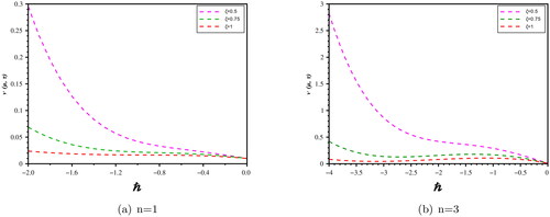Figure 3 presents the behaviour of approximate solution of (31) with n at $\eta =o.1$ and $\tau =0.5.$ Figure 4(a–d) explores the $\hslash$-curves of the q-HASTM solution (31) with distinct values of n at $\eta =o.1$ and $\tau =0.5,$ which helps to adjust the convergence region.

Figure 1. Comparison of the approximate solution of Problem 1 for distinct values ζ w.r.t. the exact solution and absolute error $|{\nu }_{\mathit{exa}.}(\eta ,\tau )-{\nu }_{\mathit{app}.}(\eta ,\tau )|$ with n = 1, $\zeta =1,,$ and $\hslash =-1..$

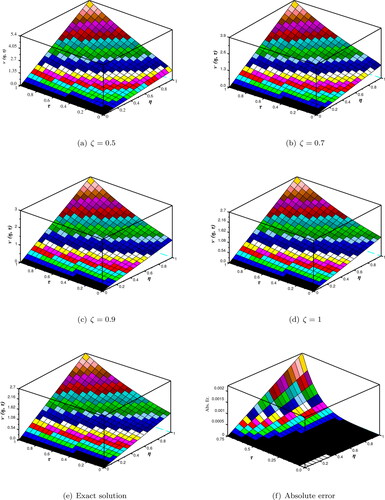
Figure 2. Comparison between the approximate solution at $\zeta \le 1$ and the exact solution with $\hslash =-1,$ n = 1, and η = 1 for Problem 1.

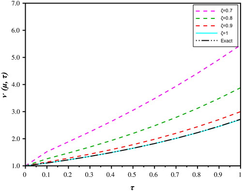
Figure 3. n-curves of $\nu (\eta ,\tau )$ for distinct values of ζ with $\hslash =-1,\eta =0.1,$ and $\tau =0.5$ for Problem 1.

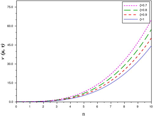
Figure 4. The $\hslash$-curves of $\nu (\eta ,\tau )$ for distinct values n with $\eta =0.1,$ and $\tau =0.5$ for Problem 1.

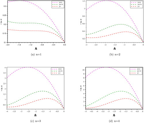
Table 1. q-Homotopy analysis Shehu transform method for $\nu (\eta ,\tau )$ in comparison with RPSM (Wang et al., 2019), HATM (Wang et al., 2019), and HPTM (Singh & Kumar, 2018) at $\hslash$ = −1, ζ = 1, and n = 1 for Problem 1.

$(\eta ,\tau )$	$|{\nu }_{\mathit{exa}.}-{\nu }_{\mathit{RPSM}}|$	$|{\nu }_{\mathit{exa}.}-{\nu }_{\mathit{HATM}}|$	$|{\nu }_{\mathit{exa}.}-{\nu }_{\mathit{HPTM}}|$	$|{\nu }_{\mathit{exa}.}-{\nu }_{q-\mathit{HASTM}}|$
(0.25, 0.25)	2.122401E − 06	2.122401E − 06	2.122401E − 06	2.122401E − 06
(0.25, 0.50)	7.094268E − 05	7.094268E − 05	7.094268E − 05	7.094268E − 05
(0.25, 0.75)	5.634807E − 04	5.634807E − 04	5.634807E − 04	5.634807E − 04
(0.25, 1.00)	2.487124E − 03	2.487124E − 03	2.487124E − 03	2.487124E − 03
(0.50, 0.25)	4.244802E − 06	4.244802E − 06	4.244802E − 06	4.244802E − 06
(0.50, 0.50)	1.418854E − 04	1.418854E − 04	1.418854E − 04	1.418854E − 04
(0.50, 0.75)	1.126961E − 03	1.126961E − 03	1.126961E − 03	1.126961E − 03
(0.50, 1.00)	4.974248E − 03	4.974248E − 03	4.974248E − 03	4.974248E − 03
(0.75, 0.25)	6.367203E − 06	6.367203E − 06	6.367203E − 06	6.367203E − 06
(0.75, 0.50)	2.128280E − 04	2.128280E − 04	2.128280E − 04	2.128280E − 04
(0.75, 0.75)	1.690442E − 03	1.690442E − 03	1.690442E − 03	1.690442E − 03
(0.75, 1.00)	7.461371E − 03	7.461371E − 03	7.461371E − 03	7.461371E − 03

Table 2 q-Homotopy analysis Shehu transform method for $\nu (\eta ,\tau )$ in comparison with RPSM (Wang et al., 2019), HATM (Wang et al., 2019), and HPTM (Singh & Kumar, 2018) at $\hslash$ = −1, ζ = 1, and n = 1 for Problem 2.

$(\eta ,\tau )$	$|{\nu }_{\mathit{exa}.}-{\nu }_{\mathit{RPSM}}|$	$|{\nu }_{\mathit{exa}.}-{\nu }_{\mathit{HATM}}|$	$|{\nu }_{\mathit{exa}.}-{\nu }_{\mathit{HPTM}}|$	$|{\nu }_{\mathit{exa}.}-{\nu }_{q-\mathit{HASTM}}|$
(0.25, 0.25)	5.300000E − 07	5.300000E − 07	5.300000E − 07	5.300000E − 07
(0.25, 0.50)	1.773500E − 05	1.773500E − 05	1.773500E − 05	1.773500E − 05
(0.25, 0.75)	1.408702E − 04	1.408702E − 04	1.408702E − 04	1.408702E − 04
(0.25, 1.00)	6.217800E − 04	6.217800E − 04	6.217800E − 04	6.217800E − 04
(0.50, 0.25)	2.123000E − 06	2.123000E − 06	2.123000E − 06	2.123000E − 06
(0.50, 0.50)	7.094300E − 05	7.094300E − 05	7.094300E − 05	7.094300E − 05
(0.50, 0.75)	5.634830E − 04	5.634830E − 04	5.634830E − 04	5.634830E − 04
(0.50, 1.00)	2.487123E − 03	2.487123E − 03	2.487123E − 03	2.487123E − 03
(0.75, 0.25)	4.776000E − 06	4.776000E − 06	4.776000E − 06	4.776000E − 06
(0.75, 0.50)	1.596200E − 04	1.596200E − 04	1.596200E − 04	1.596200E − 04
(0.75, 0.75)	1.267830E − 03	1.267830E − 03	1.267830E − 03	1.267830E − 03
(0.75, 1.00)	5.596030E − 03	5.596030E − 03	5.596030E − 03	5.596030E − 03

Moreover, Figure 5 represents the behaviour of approximate solution at distinct ζ in comparison with the exact solution and the absolute error for Problem 2. Figure 6 presents the behaviour of approximate solution with various ζ and exact solution of (44). Figure 7 explores nature of the q-HASTM solution with distinct ζ. Figure 8(a,b) explores the $\hslash$-curves of the q-HASTM solution (44) with distinct values of n at $\eta =o.1$ and $\tau =0.5,$ which helps to adjust the convergence region.

Figure 5. Comparison of approximate solution of Problem 2 for distinct values ζ w.r.t. the exact solution and absolute error $|{\nu }_{\mathit{exa}.}(\eta ,\tau )-{\nu }_{\mathit{app}.}(\eta ,\tau )|$ with n = 1, $\zeta =1,,$ and $\hslash =-1..$

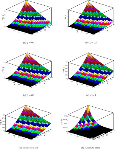
Figure 6. Comparison between the approximate solution at $\zeta \le 1$ and the exact solution with $\hslash =-1,$ n = 1, and η = 1 for Problem 2.

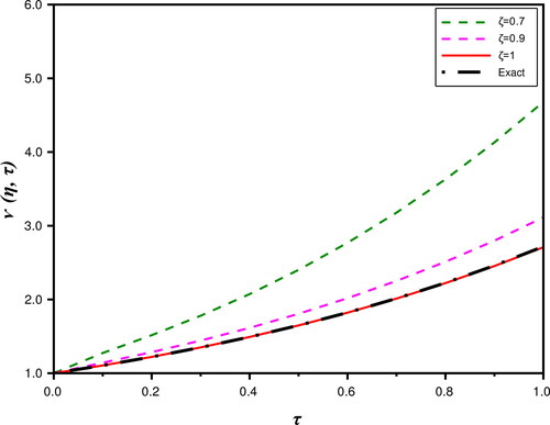
Figure 7. n-curves of $\nu (\eta ,\tau )$ for distinct values of ζ with $\hslash =-1,\eta =0.1,$ and $\tau =0.5$ for Problem 2.

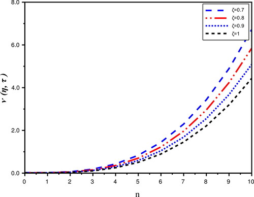
Figure 8. The $\hslash$-curves of $\nu (\eta ,\tau )$ for distinct values n with $\eta =0.1,$ and $\tau =0.5$ for Problem 2.

7. Conclusions

In this article, we successfully implemented q-HASTM to find the analytical and numerical solutions of time-fractional partial differential equations (TFPDEs). We obtained the analytical and numerical solutions of two applications of TFPDEs to present the effectiveness and accuracy of proposed scheme. Moreover, the q-homotopy analysis transform method provided the convergent series solution with easily determinable components without using any perturbation, linearization or limiting assumption. If we assume $\hslash =-1,$ and n = 1 in q-HASTM solution, then the q-HASTM solution presented an excellent agreement with the exact solution of TFPDEs. The numerical and graphical solutions obtained by q-HASTM are presented that the proposed technique is computationally very accurate and attractive technique to obtain and investigate the solutions of time fractional partial differential equations.

Authors’ contributions

The authors contributed equally and significantly in writing this paper. All authors read and approved the final manuscript.

Acknowledgements

The authors are grateful to the editor and reviewers for their thorough review and comments, which contributed to improving this article.

Disclosure statement

No potential conflict of interest was reported by the author(s).

References

- Akinyemi, L., Şenol, M., & Osman, M. S. (2022). Analytical and approximate solutions of nonlinear Schrödinger equation with higher dimension in the anomalous dispersion regime. Journal of Ocean Engineering and Science, 7(2), 143–154. doi:10.1016/j.joes.2021.07.006
- Ali, K. K., Abd El Salam, M. A., Mohamed, E., Samet, B., Kumar, S., & Osman, M. S. (2020). Numerical solution for generalized nonlinear fractional integro-differential equations with linear functional arguments using Chebyshev series. Advances in Difference Equations, 2020(1), 494. doi:10.1186/s13662-020-02951-z
- Ali, K. K., Osman, M. S., Baskonus, H. M., Elazabb, N. S., & İlhan, E. (2020). Analytical and numerical study of the HIV-1 infection of CD4+ T-cells conformable fractional mathematical model that causes acquired immunodeficiency syndrome with the effect of antiviral drug therapy. Mathematical Methods in the Applied Sciences, 1–17. doi:10.1002/mma.7022
- Al-Smadi, M., Arqub, O. A., & El-Ajou, A. (2014). A numerical iterative method for solving systems of first-order periodic boundary value problems. Journal of Applied Mathematics, 2014, 135465. doi:10.1155/2014/135465
- Amin, R., Mahariq, I., Shah, K., Awais, M., & Elsayed, F. (2021). Numerical solution of the second order linear and nonlinear integrodifferential equations using Haar wavelet method. Arab Journal of Basic and Applied Sciences, 28(1), 12–19. doi:10.1080/25765299.2020.1863561
- Arqub, O. A., Osman, M. S., Abdel-Aty, A.-H., Mohamed, A.-B. A., & Momani, S. (2020). A numerical algorithm for the solutions of ABC singular Lane–Emden type models arising in astrophysics using reproducing kernel discretization method. Mathematics, 8(6), 923. doi:10.3390/math8060923
- Bayones, F. S., Nisar, K. S., Khan, K. A., Raza, N., Hussien, N. S., Osman, M. S., & Abualnaja, K. M. (2021). Magneto-hydrodynamics (MHD) flow analysis with mixed convection moves through a stretching surface. AIP Advances, 11(4), 045001. doi:10.1063/5.0047213
- Cuahutenango-Barro, B., Taneco-Hernández, M. A., Lv, Y.-P., Gómez-Aguilar, J. F., Osman, M. S., Jahanshahi, H., & Aly, A. A. (2021). Analytical solutions of fractional wave equation with memory effect using the fractional derivative with exponential kernel. Results in Physics, 25, 104148. doi:10.1016/j.rinp.2021.104148
- Dave, S., Khan, A. M., Purohit, S. D., & Suthar, D. L. (2021). Application of green synthesized metal nano-particles in photo catalytic degradation of dyes and its mathematical modelling using Caputo Fabrizio fractional derivative without singular kernel. Journal of Mathematics, 2021, 9948422. doi:10.1155/2021/9948422
- Dhawan, S., Machado, J., Brzeziński, D. W., & Osman, M. S. (2021). A Chebyshev wavelet collocation method for some types of differential problems. Symmetry, 13(4), 536. doi:10.3390/sym13040536
- Diethelm, K., & Ford, N. J. (2002). Analysis of fractional differential equations. Journal of Mathematical Analysis and Applications, 265(2), 229–248. doi:10.1006/jmaa.2000.7194
- Djennadi, S., Shawagfeh, N., & Abu Arqub, O. (2021). A fractional Tikhonov regularization method for an inverse backward and source problems in the time-space fractional diffusion equations. Chaos, Solitons and Fractals, 150, 111127. doi:10.1016/j.chaos.2021.111127
- Djennadi, S., Shawagfeh, N., Osman, M. S., Gómez-Aguilar, J. F., & Arqub, O. A. (2021). The Tikhonov regularization method for the inverse source problem of time fractional heat equation in the view of ABC-fractional technique. Physica Scripta, 96(9), 094006. doi:10.1088/1402-4896/ac0867
- El-Tawil, M. A., & Huseen, S. N. (2012). The q-homotopy analysis method. International Journal of Applied Mathematics and Mechanics, 8, 51–75.
- El-Tawil, M. A., & Huseen, S. N. (2013). On convergence of the q-homotopy analysis method. International Journal of Contemporary Mathematical Sciences, 8, 481–497. doi:10.12988/ijcms.2013.13048
- Habenom, H., & Suthar, D. L. (2020). Numerical solution for the time-fractional Fokker–Planck equation via shifted Chebyshev polynomials of the fourth kind. Advances in Difference Equation, 315, 2020. doi:10.1186/s13662-020-02779-7
- He, J. (1999). Homotopy perturbation technique. Computer Methods in Applied Mechanics and Engineering, 178(3–4), 257–262 doi:10.1016/S0045-7825(99)00018-3
- Khalid, A., Rehan, A., Nisar, K. S., & Osman, M. S. (2021). Splines solutions of boundary value problems that arises in sculpturing electrical process of motors with two rotating mechanism circuit. Physica Scripta, 96(10), 104001. doi:10.1088/1402-4896/ac0bd0
- Khan, Z. H., & Khan, W. A. (2008). N-transform-properties and applications. NUST Journal of Engineering Sciences, 1(1), 127–133.
- Kumar, S., Chauhan, R. P., Osman, M. S., & Mohiuddine, S. A. (2021). A study on fractional HIV-AIDs transmission model with awareness effect. Mathematical Methods in the Applied Sciences, 1–15. doi:10.1002/mma.7838
- Kumar, S., Kumar, R., Osman, M. S., & Samet, B. (2021). A wavelet based numerical scheme for fractional order SEIR epidemic of measles by using Genocchi polynomials. Numerical Methods for Partial Differential Equations, 37(2), 1250–1268. doi:10.1002/num.22577
- Liao, S. J. (1992). The proposed homotopy analysis technique for the solution of nonlinear problems (PhD thesis). Shanghai Jiao Tong University, Shanghai.
- Liao, S. J. (1995). An approximate solution technique not depending on small parameters: A special example. International Journal of Non-Linear Mechanics, 30(3), 371–380. doi:10.1016/0020-7462(94)00054-E
- Maitama, S., & Zhao, W. (2019a). New Laplace-type integral transform for solving steady heat-transfer problem. Thermal Science, 25(1 Part A), 1–12. doi:10.2298/TSCI180110160M
- Maitama, S., & Zhao, W. (2019b). New integral transform: Shehu transform a generalization of Sumudu and Laplace transform for solving differential equations. International Journal of Analysis and Applications, 17(2), 167–190.
- Mistry, L., Khan, A. M., & Suthar, D. L. (2020). An epidemic slia mathematical model with Caputo Fabrizio fractional derivative. Test Engineering and Management, 83, 26374–26391.
- Nisar, K. S., Ciancio, A., Ali, K. K., Osman, M. S., Cattani, C., Baleanu, D., … Azeem, M. (2022). On beta-time fractional biological population model with abundant solitary wave structures. Alexandria Engineering Journal, 61(3), 1996–2008. doi:10.1016/j.aej.2021.06.106
- Oldham, K. B., & Spanier, J. (1974). The fractional calculus theory and applications of differentiation and integration to arbitrary order. New York: Academic Press.
- Pareek, N., Gupta, A., Agarwal, G., & Suthar, D. L. (2021). Natural transform along with HPM technique for solving fractional ADE. Advances in Mathematical Physics, 2021, 9915183. doi:10.1155/2021/9915183
- Ramani, P., Khan, A. M., Suthar, D. L. , Kumar, D. ( 2022). Approximate analytical solution for non-linear Fitzhugh–Nagumo equation of time fractional order through fractional reduced differential transform method. International Journal of Applied and Computational Mathematics, 8(1), 1–12. doi:https://doi.org/10.1007/s40819-022-01254-z
- Ramani, P., Khan, A. M., & Suthar, D. L. (2019). Revisiting analytical-approximate solution of time fractional Rosenau–Hyman equation via fractional reduced differential transform method. International Journal on Emerging Technologies, 10(2), 403–409.
- Sakar, M. G., Uludag, F., & Erdogan, F. (2016). Numerical solution of time-fractional nonlinear pdes with proportional delays by homotopy perturbation method. Applied Mathematical Modelling, 40(13–14), 6639–6649 doi:10.1016/j.apm.2016.02.005
- Singh, B. K., & Kumar, P. (2018). Homotopy perturbation transform method for solving fractional partial differential equations with proportional delay. SeMA Journal, 75(1), 111–125. doi:10.1007/s40324-017-0117-1
- Spiegel, M. R. (1965). Theory and problems of Laplace transform. Schaum’s outline series. New York: McGraw-Hill.
- Wang, L., Wu, Y., Ren, Y., & Chen, X. (2019). Two analytical methods for fractional partial differential equations with proportional delay. IAENG International Journal of Applied Mathematics, 49(1), 1–6.
- Watugala, G. K. (1998). Sumudu transform a new integral transform to solve differential equations and control engineering problems. Mathematical Engineering in Industries, 6(1), 319–329.
- Yang, X. J. (2016). A new integral transform method for solving steady heat-transfer problem. Thermal Science, 20(suppl. 3), 639–642. doi:10.2298/TSCI16S3639Y
- Yildirim, E. N., Akgül, A., & Inc, M. (2021). Reproducing kernel method for the solutions of non-linear partial differential equations. Arab Journal of Basic and Applied Sciences, 28(1), 80–86. doi:10.1080/25765299.2021.1891678