Numerical solution of unsteady state fractional advection–dispersion equation

Abstract

In this article, we find the numerical solution of unsteady state fractional order advection–dispersion equation. For an approximate solution of the proposed problem, we apply Laguerre spectral collocation method and the idea of finite difference method. The proposed method assisted us in reducing the fractional order unsteady state advection–dispersion equation into systems of ordinary differential equations, which we then expressed numerically using finite difference method. Finally, we used examples to test the efficacy of our method, and all of the solutions were compared to the exact solution.

Keywords:

• Laguerre spectral collocation method
• Caputo fractional derivative
• finite difference method
• advection–dispersion equations
• error analysis

1. Introduction

Fractional calculus is known to have played a very important role recently in various fields of science. In fact, it has many advantages over integer order models, including nonlinear ones, which in many cases do not work adequately. Mostly, fractional operators using various approaches turn out to be nonlocal in nature describing long term memory effects and asymptotic scaling. Although most of them are already well-studied, some of the usual features concerning the differentiation of functions fail, like the Leibniz rule, quotient rule, chain rule, the semigroup property, to name a few. These inconsistencies lead to constantly evolving the fractional derivative so that the best choice of definitions of fractional operators depends on empirical data that fit best in the theoretical model, and for this we find already a vast number of definitions for fractional derivative, including Caputo, Atangana, Riemann–Liouville, Hadamard, Caputo–Fabrizio, Grünwald derivative, and some others. Thus, it becomes unnecessary to worry about the definition of the function away from the point of interest. There are many of these definitions in the literature nowadays, but few of them are commonly used. The most popular ones are the Riemann–Liouville and the Caputo derivatives. It is very important to point out that all these fractional derivatives definitions have their advantages and disadvantages. Although these fractional derivative display great advantages, they are not applicable in all the situations. For example, the Riemann–Liouville derivative has certain disadvantages when trying to model real-world phenomena with fractional differential equations. The Riemann–Liouville derivative of a constant is not zero. In addition, if an arbitrary function is a constant at the origin, its fractional derivation has a singularity at the origin for instant exponential and Mittag–Leffler functions. Theses disadvantages reduce the field of application of the Riemann–Liouville fractional derivative. Caputo’s derivative demands higher conditions of regularity for differentiability: to compute the fractional derivative of a function in the Caputo sense, we must first calculate its derivative. Caputo derivatives are defined only for differentiable functions while functions that have no first-order derivative might have fractional derivatives of all orders less than one in the Riemann–Liouville sense. Typically, one deals with functions admitting some non-integrable singularities on a discrete set of isolated points located at finite distances from the origin. For the past 300 years, researchers have been studying fractional calculus, which generalizes the integration and differentiation of integer order to arbitrary order. Because of their non-local behaviour, fractional differential equations are well suited to describe various phenomena in the fields of engineering and science, and researchers’ growing interest in this field has led to the solution of real-world problems in this field. Furthermore, fractional derivatives can be used to mathematically model (Ali, Osman, Baskonus, Elazabb, & İlhan, 2020; Alshabanat, Jleli, Kumar, & Samet, 2020; Gao, Veeresha, Prakasha, & Baskonus, 2022; Ghanbari, Kumar, & Kumar, 2020; Kumar, Chauhan, Osman, & Mohiuddine, 2021; Mohammadi, Kumar, Rezapour, & Etemad, 2021; Veeresha, Prakasha, & Kumar, 2020) a variety of processes that exhibit memory and hereditary properties. The Newell–Whitehead–Segel and Allen–Cahn equations provide analytical and numerical solutions to mathematical biology models (Inan, Osman, Ak, & Baleanu, 2020). The application of the generalized differential transform method (Ramani, Khan, & Suthar, 2019b) to solve nonlinear partial differential equations with fractional space and time derivatives. The singularly perturbed boundary value issues for semilinear reaction-diffusion equations were explored in Yamac and Erdogan (2020). The Tikhonov regularization method (Djennadi et al., 2021) is used to solve the inverse source problem of the time fractional heat equation using the ABC-fractional technique. Using the reproducing kernel discretization method (Omar, Osman, Abdel-Aty, Mohamed, & Momani, 2020), a numerical algorithm for the solutions of ABC singular Lane–Emden type models arising in astrophysics. Now recently published papers on a novel numerical method, study (Ali, Abd El Salam, et al., 2020; Arslan, 2020; Mistry, Khan, Suthar, & Kumar, 2019; Mundewadi & Kumbinarasaiah, 2019; Rahaman, Kamrul Hasan, Ali, & Shamsul Alam, 2021; Sabir Wahab, Javeed, & Baskonus, 2021) for solving non-linear fractional differential equations and generalized nonlinear fractional integro-differential equations with linear functional arguments.

The advection–dispersion equation (ADE) is used in the study of solute transport (Ghosh, Kundu, & Kumar, 2021) or Brownian motion of particles in a fluid that occurs when advection and particle dispersion occur at the same time. In anomalous diffusion (Kumar, Ghosh, Jleli, & Araci, 2020), the solute transport is faster or faster than the time’s inferred square root given by Baeumer, Benson, and Meerschaert (2005). Fractional ADE better characterizes the phenomenon of anomalous diffusion of particles in transport processes. Advection–dispersion describes how pollutants flow through groundwater at seepage velocity, with Advection referring to the movement of contaminants with accompanying groundwater and Dispersion referring to a process triggered by velocity changes. The preservation of mass (Doungmo Goufo, Kumar, & Mugisha, 2020; Saw & Kumar, 2018) principle is used to investigate the ADE for solute transport. As a result, many scientists have been interested in fractional ADE. As a result, researchers are interested in solving the FADE in order to determine the solute concentration at a specific time and space. Pareek, Gupta, Agarwal, and Suthar (2021) investigated the use of the natural transform in conjunction with the HPM approach to solve fractional ADE.

Now a days, the usage of spectral and Haar wavelet methods (Bhrawy, 2014; Kumar, Ghosh, Kumar, & Jleli, 2021; Kumar, Kumar, Agarwal, & Samet, 2020; Kumar, Kumar, Osman, & Samet, 2021; Xiao-Yong & Junlin, 2015) is growing rapidly. While using spectral collocation methods for solving a certain problem, we can have a boost in our solution; since these methods are global in nature, have high accuracy, and exponential rate of convergence, for further reading in spectral methods (Bhrawy, Zaky, & Baleanu, 2015; Boyd, 2001; Canuto et al., 2006; Diethelm, 2010; Tatari & Haghighi, 2014). The primary goal of this work is to solve the space FADE using the Laguerre collocation method and the finite difference scheme.

The present paper is structured as follows: we began with classical definitions, concepts and notations of fractional calculus in Section 2; consequently, in Section 3, we introduced fundamental properties of the proposed method i.e. Laguerre spectral collocation method. In Section 4, we have given numerical examples to testify the efficiency of our method. Finally, some concluding remarks are presented in Section 5.

2. Preliminaries and notations

Definition 1.

The Caputo fractional derivative operator $D^{\gamma }$ of order γ is given by Kilbas, Srivastava, and Trujillo (2006) as follows: (1) $$D^{\gamma }f\left(x\right)=\frac{1}{\Gamma \left(n-\gamma \right)}{\int }_0^x\frac{f^{\left(n\right)}\left(t\right)}{{\left(x-t\right)}^{\left(\gamma -n+1\right)}}dt,(n-1<\gamma \le n,n\in \mathbb{N},x>0).$$(1)

Some of the properties for the fractional derivative in Caputo sense are provided by: (2) $$D^{\gamma }\left({\gamma }_{1}p\left(x\right)+{\gamma }_{2}q\left(x\right)\right)={\gamma }_1{D}^{\gamma }p\left(x\right)+{\gamma }_2{D}^{\gamma }q\left(x\right),({\gamma }_1,{\gamma }_2\in ℝ),$$(2) where γ₁ and γ₂ are constants, and the notation $\lceil \gamma \rceil$ denotes the smallest integer greater than or equal to γ, and ${\mathbb{N}}_0=\left\{0,1,2,\dots \right\}.$ (3) $$D^{\gamma }C=0,$$(3)

C is a constant. (4) $$D^{\gamma }{x}^{\sigma }=\{\begin{array}{c}0,\mathit{for}\sigma \in {\mathbb{N}}_0,\mathit{and}\sigma <\lceil \gamma \rceil ,\hfill \\ \frac{\Gamma \left(\sigma +1\right)}{\Gamma \left(\sigma -\gamma +1\right)}{x}^{\sigma -\gamma },\mathit{for}\sigma \in {\mathbb{N}}_0\mathit{and}\sigma \ge \lceil \gamma \rceil .\hfill \end{array}$$(4)

The primary goal of this work is to find an approximation of an unsteady state space fractional ADE with source f(x, t) defined on (5)(5) $$\frac{\partial u\left(x,t\right)}{\partial t}=\lambda \frac{{\partial }^{\gamma }u\left(x,t\right)}{\partial x^{\gamma }}-\mu \frac{{\partial }^{\eta }u\left(x,t\right)}{\partial x^{\eta }}+f\left(x,t\right),(0<x<1,0<t\le T),$$(5) using the idea of Laguerre collocation method. (5) $$\frac{\partial u\left(x,t\right)}{\partial t}=\lambda \frac{{\partial }^{\gamma }u\left(x,t\right)}{\partial x^{\gamma }}-\mu \frac{{\partial }^{\eta }u\left(x,t\right)}{\partial x^{\eta }}+f\left(x,t\right),(0<x<1,0<t\le T),$$(5) (6) $$u\left(0,t\right)=u\left(1,t\right)=0,$$(6) (7) $$u\left(x,0\right)=\phi \left(x\right),$$(7) where $1<\gamma \le 2,0<\eta \le 1,$ μ is the average fluid velocity and λ belongs to the dispersion coefficient.

3. The properties and fractional derivatives of Laguerre polynomials

The generalized Laguerre polynomial ${[L_n^{\left(v\right)}(x)]}_{n=0}^{\infty },v>-1$ defined on the interval $[0,\infty )$ and can be expressed by the recurrence relation (see also Khader, Talaat, Danaf, & Hendy, 2012) as: (8) $$\left(n+1\right)L_{n+1}^{\left(v\right)}\left(x\right)+\left(x-2n-v-1\right)L_n^{(v)}\left(x\right)+(n+v)L_{n-1}^{(v)}\left(x\right)=0,n=1,2,3,\dots$$(8) with $L_0^{(v)}\left(x\right)=1$ and $L_1^{(v)}\left(x\right)=v+1-x.$

The explicit formula of degree $\mathrm{‘}n’$ Laguerre polynomial is: (9) $$L_n^{(v)}\left(x\right)=\sum _{k=0}^n\frac{{(-1)}^k}{k!}\left(\begin{array}{c}n+v\\ n-k\end{array}\right)x^k=\left(\begin{array}{c}n+v\\ n\end{array}\right)\sum _{k=0}^n\frac{{(-n)}_k}{{\left(v+1\right)}_k}\frac{x^k}{k!},$$(9) i.e., ${(v)}_0=1,{(v)}_k=v(v+1)(v+2)\dots (v+k-1),k=1,2,3,\dots$ and $L_n^{(v)}\left(0\right)=\left(\begin{array}{c}n+v\\ n\end{array}\right).$ These degree $\mathrm{‘}n’$ Laguerre polynomials with respect to the weight function $\varphi (x)=\frac{1}{\Gamma \left(1+v\right)}{x}^v{e}^{-x}$ are orthogonal on the interval $[0,\infty )$ and its orthogonality relation is defined as: (10) $$\frac{1}{\Gamma \left(1+v\right)}{\int }_0^{\infty }{x}^v{e}^{-x}{L}_m^{(v)}\left(x\right)L_n^{(v)}\left(x\right)dx=\left(\begin{array}{c}n+v\\ n\end{array}\right){\delta }_{mn}.$$(10)

Satisfying the differentiation formula as below (11) $$D^k{L}_n^{(v)}\left(x\right)={(-1)}^k{L}_{n-k}^{(v+k)}\left(x\right),k=0,1,\dots ,n.$$(11)

Consider u(x) be a square integrable function on the semi-infinite interval $[0,\infty ).$ The function u(x) can also be extended in relation of the weight function. (12) $$u\left(x\right)=\sum _{i=0}^{\infty }{\omega }_i{L}_i^{\left(v\right)}\left(x\right),$$(12) and ω_i can be expressed as: (13) $${\omega }_i=\frac{\Gamma \left(i+1\right)}{\Gamma \left(i+v+1\right)}{\int }_0^{\infty }{x}^v{e}^{-x}{L}_i^{\left(v\right)}\left(x\right)u(x)dx,i=0,1,2,\dots$$(13)

For a possible mathematical manipulation, we only consider the first $\left(m+1\right)$ terms of the above (12)(12) $$u\left(x\right)=\sum _{i=0}^{\infty }{\omega }_i{L}_i^{\left(v\right)}\left(x\right),$$(12) Laguerre series: (14) $$u_m\left(x\right)=\sum _{i=0}^m{\omega }_i{L}_i^{\left(v\right)}\left(x\right).$$(14)

Theorem 3.1.

Let $\gamma >0$ and $u_m\left(x\right)$ be an approximate function based on Laguerre polynomials, then: (15) $$D^{\gamma }\left(u_m\left(x\right)\right)\cong \sum _{i=\lceil \gamma \rceil }^m\sum _{k=\lceil \gamma \rceil }^i{\omega }_i{\psi }_{i,k}^{\left(\gamma \right)}{x}^{k-\gamma },$$(15) where (16) $${\psi }_{i,k}^{\left(\gamma \right)}=\frac{{\left(-1\right)}^k}{\Gamma \left(k+1-\gamma \right)}\left(\begin{array}{c}i+v\hfill \\ i-k\hfill \end{array}\right).$$(16)

Proof.

Based on linearity property of Caputo’s fractional derivative, we arrive at: (17) $$D^{\gamma }\left(u_m\left(x\right)\right)=\sum _{i=0}^m{\omega }_i{D}^{\gamma }\left(L_i^{(v)}\left(x\right)\right).$$(17)

Using Equations (3)(3) $$D^{\gamma }C=0,$$(3) and (4)(4) $$D^{\gamma }{x}^{\sigma }=\{\begin{array}{c}0,\mathit{for}\sigma \in {\mathbb{N}}_0,\mathit{and}\sigma <\lceil \gamma \rceil ,\hfill \\ \frac{\Gamma \left(\sigma +1\right)}{\Gamma \left(\sigma -\gamma +1\right)}{x}^{\sigma -\gamma },\mathit{for}\sigma \in {\mathbb{N}}_0\mathit{and}\sigma \ge \lceil \gamma \rceil .\hfill \end{array}$$(4) , we get: (18) $$D^{\gamma }\left(L_i^{(v)}\left(x\right)\right)=0,i=0,1,\dots ,\lceil \gamma \rceil -1,\gamma >0.$$(18)

Also, for $i=\lceil \gamma \rceil ,\dots ,m,$ by using Equations (3)(3) $$D^{\gamma }C=0,$$(3) and (4)(4) $$D^{\gamma }{x}^{\sigma }=\{\begin{array}{c}0,\mathit{for}\sigma \in {\mathbb{N}}_0,\mathit{and}\sigma <\lceil \gamma \rceil ,\hfill \\ \frac{\Gamma \left(\sigma +1\right)}{\Gamma \left(\sigma -\gamma +1\right)}{x}^{\sigma -\gamma },\mathit{for}\sigma \in {\mathbb{N}}_0\mathit{and}\sigma \ge \lceil \gamma \rceil .\hfill \end{array}$$(4) , we get: (19) $$\begin{array}{c}{D}^{\gamma }\left(L_i^{(v)}\left(x\right)\right)=\sum _{k=0}^i\frac{{(-1)}^k}{k!}\left(\begin{array}{c}i+v\\ i-k\end{array}\right)D^{\gamma }\left\{x^k\right\}\hfill \\ =\sum _{k=\lceil \gamma \rceil }^i\frac{{(-1)}^k}{\Gamma \left(k+1-\gamma \right)}\left(\begin{array}{c}i+v\\ i-k\end{array}\right)x^{k-\gamma }.\hfill \end{array}$$(19)

From Equations (17)–(19): (20) $$D^{\gamma }\left(u_m\left(x\right)\right)=\sum _{i=\lceil \gamma \rceil }^m\sum _{k=\lceil \gamma \rceil }^i{\omega }_i\frac{{(-1)}^k}{\Gamma \left(k+1-\gamma \right)}\left(\begin{array}{c}i+v\\ i-k\end{array}\right)x^{k-\gamma }.$$(20)

Rearranging (20)(20) $$D^{\gamma }\left(u_m\left(x\right)\right)=\sum _{i=\lceil \gamma \rceil }^m\sum _{k=\lceil \gamma \rceil }^i{\omega }_i\frac{{(-1)}^k}{\Gamma \left(k+1-\gamma \right)}\left(\begin{array}{c}i+v\\ i-k\end{array}\right)x^{k-\gamma }.$$(20) , we arrive at (15)(15) $$D^{\gamma }\left(u_m\left(x\right)\right)\cong \sum _{i=\lceil \gamma \rceil }^m\sum _{k=\lceil \gamma \rceil }^i{\omega }_i{\psi }_{i,k}^{\left(\gamma \right)}{x}^{k-\gamma },$$(15) . □

2.1. Error analysis

Theorem 3.2.

Suppose the $\left(m+1\right)$ continuously differentiable function $h\left(x\right)$ is defined on the semi-infinite interval $[0,\infty )$ and $u_m(x)={\sum }_{i=0}^m{\omega }_i{L}_i^{\left(-0.5\right)}\left(x\right)$ be best approximate function square of $h\left(x\right)$, then: (21) $$\Vert h\left(x\right)-u_m\left(x\right)\Vert \le \frac{M{S}^{m+1}}{\left(m+1\right)!},$$(21)

Where $M={\max }_{x\in [0,\infty )}{h}^{\left(m+1\right)}\left(x\right)$ and $S=\max \left[x_0,x-x_0\right].$

Proof.

Consider the Taylor polynomial: (22) $$h\left(x\right)=h\left(x_0\right)+h^{\prime }\left(x_0\right)\frac{\left(x-x_0\right)}{1!}+\cdots +h^{\left(m\right)}\left(x_0\right)\frac{{\left(x-x_0\right)}^m}{m!}+h^{\left(m+1\right)}\left(\xi \right)\frac{{\left(x-x_0\right)}^{m+1}}{\left(m+1\right)!},$$(22) where $x_0\in [0,\infty )$ and $\xi \in \left[x_0,x\right].$

We assume that (23) $$p_m\left(x\right)=h\left(x_0\right)+h^{\prime }\left(x_0\right)\frac{\left(x-x_0\right)}{1!}+\cdots +h^{\left(m\right)}\left(x_0\right)\frac{{\left(x-x_0\right)}^m}{m!}.$$(23)

Hence, (24) $$\left|h\left(x\right)-p_m\left(x\right)\right|=\left|h^{\left(m+1\right)}\left(\xi \right)\frac{{\left(x-x_0\right)}^{m+1}}{\left(m+1\right)!}\right|,$$(24) $$\begin{array}{c}{\left|\left|h\left(x\right)-u_m\left(x\right)\right|\right|}^2\le {\left|\left|h\left(x\right)-p_m\left(x\right)\right|\right|}^2\hfill \\ ={\int }_0^{\infty }\varphi \left(x\right){\left[h\left(x\right)-p_m\left(x\right)\right]}^{2}dx\hfill \\ ={\int }_0^{\infty }\varphi \left(x\right){\left[h^{\left(m+1\right)}\left(\xi \right)\frac{{\left(x-x_0\right)}^{m+1}}{\left(m+1\right)!}\right]}^{2}dx\hfill \\ \le \frac{M^2}{{\left[\left(m+1\right)!\right]}^2}{\int }_0^{\infty }\varphi \left(x\right){\left(x-x_0\right)}^{2m+2}dx\hfill \\ =\frac{M^2}{{\left[\left(m+1\right)!\right]}^2}{\int }_0^{\infty }{\left(x-x_0\right)}^{2m+2}\frac{1}{\Gamma \left(0.5\right)}{x}^{-0.5}{e}^{-x}dx.\hfill \end{array}$$

Hence $S=\max \left[x_0.x-x_0\right],$ we have $${\left|\left|h\left(x\right)-u_m\left(x\right)\right|\right|}^2\le \frac{M^2{S}^{2m+2}}{{\left[\left(m+1\right)!\right]}^2}\frac{1}{\Gamma \left(0.5\right)}{\int }_0^{\infty }{x}^{-0.5}{e}^{-x}dx=\frac{M^2{S}^{2m+2}}{{\left[\left(m+1\right)!\right]}^2}.$$

Taking square root both sides, we get $$\left|\left|h\left(x\right)-u_m\left(x\right)\right|\right|\le \frac{M{S}^{m+1}}{\left(m+1\right)!}.$$

4. Numerical examples

Example 1.

Take a look at the space fractional ADE below. (25) $$\frac{\partial u\left(x,t\right)}{\partial t}=\frac{{\partial }^{\gamma }u\left(x,t\right)}{\partial x^{\gamma }}-\frac{{\partial }^{\eta }u\left(x,t\right)}{\partial x^{\eta }}+f\left(x,t\right),(0<x<1,0<t\le T,1<\gamma \le 2,0<\eta \le 1),$$(25) where (26) $$f\left(x,t\right)=e^{\left(-2t\right)}\left(2\left(x^{\eta }-x^{\gamma }\right)-\gamma !+\frac{\Gamma \left(\gamma +1\right)}{\Gamma \left(\gamma -\eta +1\right)}{x}^{\gamma -\eta }-\eta !\right),$$(26) consider the following initial and boundary conditions (27) $$u\left(0,t\right)=u\left(1,t\right)=0,$$(27) (28) $$u\left(x,0\right)=x^{\gamma }-x^{\eta }.$$(28)

For comparison, the exact solution of our proposed problem is $u\left(x,t\right)=e^{-2t}\left(x^{\gamma }-x^{\eta }\right).$

To use the Laguerre collocation method, we approximate it with m = 4. (29) $$u_4\left(x,t\right)=\sum _{i=0}^4{u}_i\left(t\right)L_i^{\left(v\right)}\left(x\right).$$(29)

Adopting Theorem 3.1 and Equation (29)(29) $$u_4\left(x,t\right)=\sum _{i=0}^4{u}_i\left(t\right)L_i^{\left(v\right)}\left(x\right).$$(29) on (25)(25) $$\frac{\partial u\left(x,t\right)}{\partial t}=\frac{{\partial }^{\gamma }u\left(x,t\right)}{\partial x^{\gamma }}-\frac{{\partial }^{\eta }u\left(x,t\right)}{\partial x^{\eta }}+f\left(x,t\right),(0<x<1,0<t\le T,1<\gamma \le 2,0<\eta \le 1),$$(25) , we get: (30) $$\begin{array}{c}\sum _{i=0}^4\frac{d{u}_i\left(t\right)}{dt}{L}_i^{\left(v\right)}\left(x_p\right)\\ =\sum _{i=\lceil \gamma \rceil }^4\sum _{k=\lceil \gamma \rceil }^i{u}_i\left(t\right){\psi }_{i,k}^{\left(\gamma \right)}{x}_p{}^{k-\gamma }-\sum _{i=\lceil \eta \rceil }^4\sum _{k=\lceil \eta \rceil }^i{u}_i\left(t\right){\psi }_{i,k}^{\left(\eta \right)}{x}_p{}^{k-\eta }+f\left(x_p,t\right),p=0,1,2,\end{array}$$(30) where x_p’s are the roots of Laguerre polynomials. To arrive at the systems of ordinary differential equations we substituted Equation (29)(29) $$u_4\left(x,t\right)=\sum _{i=0}^4{u}_i\left(t\right)L_i^{\left(v\right)}\left(x\right).$$(29) on (27)(27) $$u\left(0,t\right)=u\left(1,t\right)=0,$$(27) and using Equation (30)(30) $$\begin{array}{c}\sum _{i=0}^4\frac{d{u}_i\left(t\right)}{dt}{L}_i^{\left(v\right)}\left(x_p\right)\\ =\sum _{i=\lceil \gamma \rceil }^4\sum _{k=\lceil \gamma \rceil }^i{u}_i\left(t\right){\psi }_{i,k}^{\left(\gamma \right)}{x}_p{}^{k-\gamma }-\sum _{i=\lceil \eta \rceil }^4\sum _{k=\lceil \eta \rceil }^i{u}_i\left(t\right){\psi }_{i,k}^{\left(\eta \right)}{x}_p{}^{k-\eta }+f\left(x_p,t\right),p=0,1,2,\end{array}$$(30) : (31) $$u_0^{\prime }\left(t\right)+R_1{u}_1^{\prime }\left(t\right)+R_2{u}_2^{\prime }\left(t\right)+R_3{u}_3^{\prime }\left(t\right)+R_4{u}_4^{\prime }\left(t\right)=G_1{u}_1\left(t\right)+G_2{u}_2\left(t\right)+G_3{u}_3\left(t\right)+G_4{u}_4\left(t\right)+f_0\left(t\right),$$(31) (32) $$u_0^{\prime }\left(t\right)+K_1{u}_1^{\prime }\left(t\right)+K_2{u}_2^{\prime }\left(t\right)+K_3{u}_3^{\prime }\left(t\right)+K_4{u}_4^{\prime }\left(t\right)=H_1{u}_1\left(t\right)+H_2{u}_2\left(t\right)+H_3{u}_3\left(t\right)+H_4{u}_4\left(t\right)+f_1\left(t\right),$$(32) (33) $$u_0^{\prime }\left(t\right)+S_1{u}_1^{\prime }\left(t\right)+S_2{u}_2^{\prime }\left(t\right)+S_3{u}_3^{\prime }\left(t\right)+S_4{u}_4^{\prime }\left(t\right)=T_1{u}_1\left(t\right)+T_2{u}_2\left(t\right)+T_3{u}_3\left(t\right)+T_4{u}_4\left(t\right)+f_2\left(t\right),$$(33) (34) $$\begin{array}{c}{u}_0\left(t\right)+\left(v+1\right)u_1\left(t\right)+\frac{1}{2}\left(v+2\right)\left(v+1\right)u_2\left(t\right)+\frac{1}{6}\left(v+3\right)\left(v+2\right)\left(v+1\right)u_3\left(t\right)\hfill \\ +\frac{1}{24}\left(v+4\right)\left(v+3\right)\left(v+2\right)\left(v+1\right)u_3\left(t\right)=0,\hfill \end{array}$$(34) (35) $$u_0\left(t\right)+L_1^{\left(v\right)}\left(1\right)u_1\left(t\right)+L_2^{\left(v\right)}\left(1\right)u_2\left(t\right)+L_3^{\left(v\right)}\left(1\right)u_3\left(t\right)+L_4^{\left(v\right)}\left(1\right)u_4\left(t\right)=0,$$(35) such that: $$\begin{array}{c}{R}_1=L_1^{\left(v\right)}\left(x_0\right),R_2=L_2^{\left(v\right)}\left(x_0\right),R_3=L_3^{\left(v\right)}\left(x_0\right),R_4=L_4^{\left(v\right)}\left(x_0\right),\\ G_1=-{\psi }_{1,1}^{\left(\eta \right)}{x}_0{}^{1-\eta },\\ G_2=\left\{{\psi }_{2,2}^{\left(\gamma \right)}{x}_0{}^{2-\gamma }-\left({\psi }_{2,1}^{\left(\eta \right)}{x}_0{}^{1-\eta }+{\psi }_{2,2}^{\left(\eta \right)}{x}_0{}^{2-\eta }\right)\right\},\\ G_3=\left\{{\psi }_{3,3}^{\left(\gamma \right)}{x}_0{}^{3-\gamma }+{\psi }_{3,2}^{\left(\gamma \right)}{x}_0{}^{2-\gamma }-\left({\psi }_{3,3}^{\left(\eta \right)}{x}_0{}^{3-\eta }+{\psi }_{3,2}^{\left(\eta \right)}{x}_0{}^{2-\eta }+{\psi }_{3,1}^{\left(\eta \right)}{x}_0{}^{1-\eta }\right)\right\},\\ G_4=\left\{{\psi }_{4,4}^{\left(\gamma \right)}{x}_0{}^{4-\gamma }+{\psi }_{4,3}^{\left(\gamma \right)}{x}_0{}^{3-\gamma }+{\psi }_{4,2}^{\left(\gamma \right)}{x}_0{}^{2-\gamma }-\left({\psi }_{4,4}^{\left(\eta \right)}{x}_0{}^{4-\eta }+{\psi }_{4,3}^{\left(\eta \right)}{x}_0{}^{3-\eta }+{\psi }_{4,2}^{\left(\eta \right)}{x}_0{}^{2-\eta }+{\psi }_{4,1}^{\left(\eta \right)}{x}_0{}^{1-\eta }\right)\right\},\\ K_1=L_1^{\left(v\right)}\left(x_1\right),K_2=L_2^{\left(v\right)}\left(x_1\right),K_3=L_3^{\left(v\right)}\left(x_1\right),K_4=L_4^{\left(v\right)}\left(x_1\right),\\ H_1=-{\psi }_{1,1}^{\left(\eta \right)}{x}_1{}^{1-\eta },H_2=\left\{{\psi }_{2,2}^{\left(\gamma \right)}{x}_1{}^{2-\gamma }-\left({\psi }_{2,1}^{\left(\eta \right)}{x}_1{}^{1-\eta }+{\psi }_{2,2}^{\left(\eta \right)}{x}_1{}^{2-\eta }\right)\right\},\\ H_3=\left\{{\psi }_{3,3}^{\left(\gamma \right)}{x}_1{}^{3-\gamma }+{\psi }_{3,2}^{\left(\gamma \right)}{x}_1{}^{2-\gamma }-\left({\psi }_{3,3}^{\left(\eta \right)}{x}_1{}^{3-\eta }+{\psi }_{3,2}^{\left(\eta \right)}{x}_1{}^{2-\eta }+{\psi }_{3,1}^{\left(\eta \right)}{x}_1{}^{1-\eta }\right)\right\},\\ H_4=\left\{{\psi }_{4,4}^{\left(\gamma \right)}{x}_1{}^{4-\gamma }+{\psi }_{4,3}^{\left(\gamma \right)}{x}_1{}^{3-\gamma }+{\psi }_{4,2}^{\left(\gamma \right)}{x}_1{}^{2-\gamma }-\left({\psi }_{4,4}^{\left(\eta \right)}{x}_1{}^{4-\eta }+{\psi }_{4,3}^{\left(\eta \right)}{x}_1{}^{3-\eta }+{\psi }_{4,2}^{\left(\eta \right)}{x}_1{}^{2-\eta }+{\psi }_{4,1}^{\left(\eta \right)}{x}_1{}^{1-\eta }\right)\right\},\\ S_1=L_1^{\left(v\right)}\left(x_2\right),S_2=L_2^{\left(v\right)}\left(x_2\right),S_3=L_3^{\left(v\right)}\left(x_2\right),S_4=L_4^{\left(v\right)}\left(x_2\right),\\ T_1=-{\psi }_{1,1}^{\left(\eta \right)}{x}_2{}^{1-\eta },T_2=\left\{{\psi }_{2,2}^{\left(\gamma \right)}{x}_2{}^{2-\gamma }-\left({\psi }_{2,1}^{\left(\eta \right)}{x}_2{}^{1-\eta }+{\psi }_{2,2}^{\left(\eta \right)}{x}_2{}^{2-\eta }\right)\right\},\\ T_3=\left\{{\psi }_{3,3}^{\left(\gamma \right)}{x}_2{}^{3-\gamma }+{\psi }_{3,2}^{\left(\gamma \right)}{x}_2{}^{2-\gamma }-\left({\psi }_{3,3}^{\left(\eta \right)}{x}_2{}^{3-\eta }+{\psi }_{3,2}^{\left(\eta \right)}{x}_2{}^{2-\eta }+{\psi }_{3,1}^{\left(\eta \right)}{x}_2{}^{1-\eta }\right)\right\},\\ T_4=\left\{{\psi }_{4,4}^{\left(\gamma \right)}{x}_2{}^{4-\gamma }+{\psi }_{4,3}^{\left(\gamma \right)}{x}_2{}^{3-\gamma }+{\psi }_{4,2}^{\left(\gamma \right)}{x}_2{}^{2-\gamma }-\left({\psi }_{4,4}^{\left(\eta \right)}{x}_2{}^{4-\eta }+{\psi }_{4,3}^{\left(\eta \right)}{x}_2{}^{3-\eta }+{\psi }_{4,2}^{\left(\eta \right)}{x}_2{}^{2-\eta }+{\psi }_{4,1}^{\left(\eta \right)}{x}_2{}^{1-\eta }\right)\right\},\\ a_1=v+1,a_2=\frac{1}{2}\left(v+2\right)\left(v+1\right),a_3=\frac{1}{6}\left(v+3\right)\left(v+2\right)\left(v+1\right),a_4=\frac{1}{24}\left(v+4\right)\left(v+3\right)\left(v+2\right)\left(v+1\right),\\ b_1=L_1^{\left(v\right)}\left(1\right),b_2=L_2^{\left(v\right)}\left(1\right),b_3=L_3^{\left(v\right)}\left(1\right),b_4=L_4^{\left(v\right)}\left(1\right),\end{array}$$

Consider $T=T_{\mathit{final},}0<t_m\le T$ and $\Delta t=T/N,t_m=m\Delta t,\mathit{for}m=0,1,2,\dots ,N.$ Now, in order to solve Equations (31)–(35). We discretize the first derivatives using the idea of finite difference method (FDM). (36) $$\begin{array}{c}\frac{u_0^m-u_0^{m-1}}{\Delta t}+R_1\frac{u_1^m-u_1^{m-1}}{\Delta t}+R_2\frac{u_2^m-u_2^{m-1}}{\Delta t}+R_3\frac{u_3^m-u_3^{m-1}}{\Delta t}+R_4\frac{u_4^m-u_4^{m-1}}{\Delta t}\hfill \\ =G_1{u}_1\left(t\right)+G_2{u}_2\left(t\right)+G_3{u}_3\left(t\right)++G_4{u}_4\left(t\right)+f_0\left(t\right),\hfill \end{array}$$(36) (37) $$\begin{array}{c}\frac{u_0^m-u_0^{m-1}}{\Delta t}+K_1\frac{u_1^m-u_1^{m-1}}{\Delta t}+K_2\frac{u_2^m-u_2^{m-1}}{\Delta t}+K_3\frac{u_3^m-u_3^{m-1}}{\Delta t}+K_4\frac{u_4^m-u_4^{m-1}}{\Delta t}\hfill \\ =H_1{u}_1\left(t\right)+H_2{u}_2\left(t\right)+H_3{u}_3\left(t\right)+H_4{u}_4\left(t\right)+f_1\left(t\right),\hfill \end{array}$$(37) (38) $$\begin{array}{c}\frac{u_0^m-u_0^{m-1}}{\Delta t}+S_1\frac{u_1^m-u_1^{m-1}}{\Delta t}+S_2\frac{u_2^m-u_2^{m-1}}{\Delta t}+S_3\frac{u_3^m-u_3^{m-1}}{\Delta t}+S_4\frac{u_4^m-u_4^{m-1}}{\Delta t}\hfill \\ =T_1{u}_1\left(t\right)+T_2{u}_2\left(t\right)+T_3{u}_3\left(t\right)+T_4{u}_4\left(t\right)+f_2\left(t\right),\hfill \end{array}$$(38) (39) $$u_0^m+a_1{u}_1^m+a_2{u}_2^m+a_3{u}_3^m+a_4{u}_4^m=0,$$(39) (40) $$u_0^m+b_1{u}_1^m+b_2{u}_2^m+b_3{u}_3^m+b_4{u}_4^m=0.$$(40)

Re-arranging Equations (36)–(40), we arrive at the following matrix form: $$\begin{array}{c}\left(\begin{array}{ccccc}1& R_1-\Delta t{G}_1& R_2-\Delta t{G}_2& R_3-\Delta t{G}_3& R_4-\Delta t{G}_4\\ 1& K_1-\Delta t{H}_1& K_2-\Delta t{H}_2& K_3-\Delta t{H}_3& K_4-\Delta t{H}_4\\ 1& S_1-\Delta t{T}_1& S_2-\Delta t{T}_2& S_3-\Delta t{T}_3& S_4-\Delta t{T}_4\\ 1& a_1& a_2& a_3& a_4\\ 1& b_1& b_2& b_3& b_4\end{array}\right){\left(\begin{array}{c}{u}_0\\ u_1\\ u_2\\ u_3\\ u_4\end{array}\right)}^m\\ =\left(\begin{array}{ccccc}1& R_1& R_2& R_3& R_4\\ 1& K_1& K_2& K_3& K_4\\ 1& S_1& S_2& S_3& S_4\\ 0& 0& 0& 0& 0\\ 0& 0& 0& 0& 0\end{array}\right){\left(\begin{array}{c}{u}_0\\ u_1\\ u_2\\ u_3\\ u_4\end{array}\right)}^{m-1}+\Delta t{\left(\begin{array}{c}{f}_0\\ f_1\\ f_2\\ 0\\ 0\end{array}\right)}^m.\end{array}$$

Or, it can be written as: (41) $$A{U}^m=B{U}^{m-1}+F^m,A^{-1}A{U}^m=A^{-1}B{U}^{m-1}+A^{-1}{F}^m\iff U^m=A^{-1}B{U}^{m-1}+A^{-1}{F}^m,$$(41) where $U^m={\left(\begin{array}{cccc}{u}_0^m& u_1^m& u_2^m& \begin{array}{cc}{u}_3^m& u_4^m\end{array}\end{array}\right)}^T$ and $F^m={\left(\begin{array}{cccc}\Delta t{f}_0^m& \begin{array}{cc}\Delta t{f}_1^m& \Delta t{f}_2^m\end{array}& 0& 0\end{array}\right)}^T.$

Using the Laguerre collocation points $L_{m+1-\lceil \gamma \rceil }^{\left(-0.5\right)},$ we find the unknown coefficients (Table 1) $$x_0=0.1902,x_1=1.7845,x_2=5.5253$$

Table 1. The approximate solution, exact solution and their comparison using $T=0.4,m=4,\gamma =2,\eta =1,\Delta t=0.0005.$

x	Exact	Laguerre	Error
0	0	1.25e − 15	1.25e − 15
0.1	−4.04e − 02	−4.04e − 02	6.51e − 06
0.2	−7.19e − 02	−7.19e − 02	1.43e − 05
0.3	−9.44e − 02	−9.44e − 02	2.22e − 05
0.4	−1.08e − 01	−1.08e − 01	2.93e − 05
0.5	−1.12e − 01	−1.12e − 01	3.44e − 05
0.6	−1.08e − 01	−1.08e − 01	3.66e − 05
0.7	−9.44e − 02	−9.44e − 02	3.51e − 05
0.8	−7.19e − 02	−7.19e − 02	2.89e − 05
0.9	−4.04e − 02	−4.05e − 02	1.75e − 05
1	0	−5.28e − 09	5.28e − 09

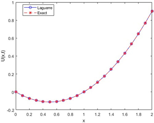
Here, we are represent approximate solution of Example 1 for different value of parameters in Figures 1–9.

Figure 1. Solution for $\gamma =1.5,\eta =0.5$ and t = 0.2.

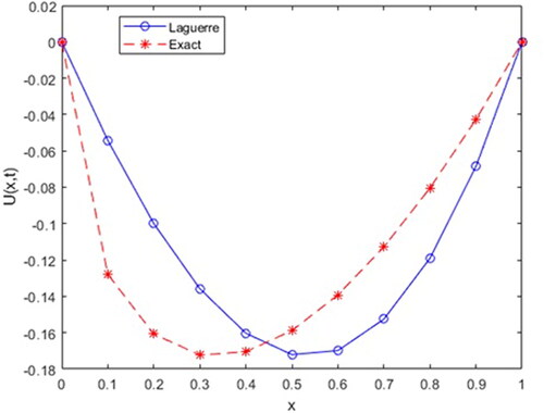
Figure 2. Solution for $\gamma =1.8,\eta =0.7$ and t = 0.2.

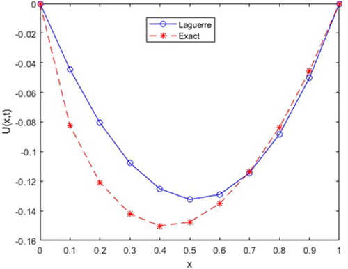
Figure 3. Solution for $\gamma =1.9,\eta =0.9$ and t = 0.2.

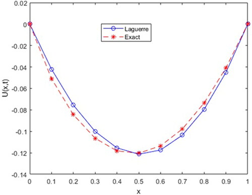
Figure 4. Solution for $\gamma =1.8,\eta =1$ and t = 0.5.

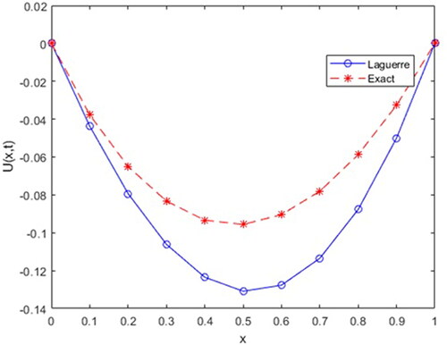
Figure 5. Solution for for $\gamma =1.9,\eta =1$ and t = 0.5.

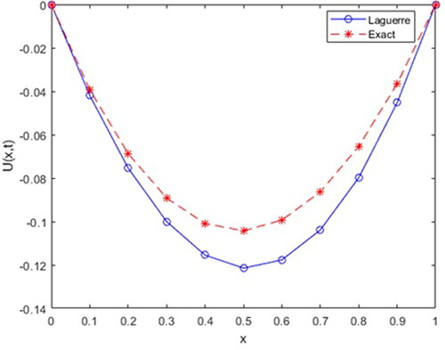
Figure 6. Solution for $\gamma =2,\eta =0.9$ and t = 0.4.

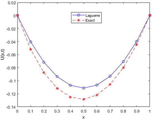
Figure 7. Solution for $\gamma =2,\eta =1$ and t = 0.4.

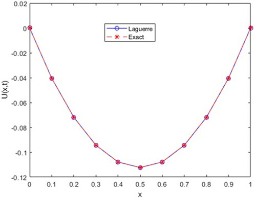
Figure 8. Solution for $\gamma =2,\eta =1$ and t = 0.4.

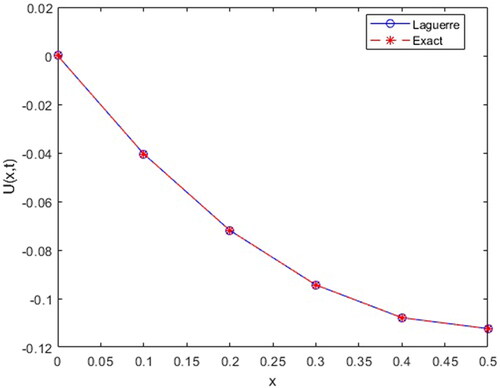
Figure 9. Solution for $\gamma =2,\eta =1$ and t = 0.4.

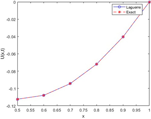
Figure 10. Solution for $\gamma =2,\eta =1$ and t = 0.4.

Example 2.

Find an approximate solution for the given unsteady state space fractional ADE subject to the initial and boundary conditions. (42) $$\frac{\partial u\left(x,t\right)}{\partial t}=\frac{{\partial }^{1.5}u\left(x,t\right)}{\partial x^{1.5}}-2\frac{\partial u\left(x,t\right)}{\partial x}+f\left(x,t\right),(0<x<1,0<t\le T),$$(42) where $f\left(x,t\right)=x\left(x-1\right)\left(2t-1\right)+2t\left(t-1\right)\left(2x-1\right)-\frac{4\sqrt{x}t\left(t-1\right)}{\sqrt{\pi }},$subject to (43) $$u\left(x,0\right)=0,$$(43) (44) $$u\left(0,t\right)=u\left(1,t\right)=0.$$(44)

For comparison, the exact solution of our proposed problem is $u\left(x,t\right)=xt\left(x-1\right)\left(t-1\right)$ (Table 2).

Table 2. The approximate solution, exact solution and their comparison using $T=0.4,m=4,\Delta t=0.0005.$

x	Exact	Laguerre	Error
0	0	3e − 20	3.46e − 20
0.1	0.008	0.008	6.59e − 06
0.2	0.014	0.014	1.08e − 05
0.3	0.019	0.019	1.32e − 05
0.4	0.022	0.022	1.39e − 05
0.5	0.023	0.022	1.33e − 05
0.6	0.022	0.022	1.16e − 05
0.7	0.019	0.019	9.25e − 06
0.8	0.014	0.014	6.35e − 06
0.9	0.008	0.008	3.19e − 06
1	0	1e − 09	1.36e − 09

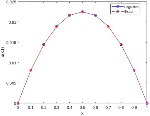
Here, we are represent approximate solution of Example 2 for parameters in Figure 11.

Figure 11. Solution for $\alpha =1.8,\beta =0.9$ and t = 0.4.

5. Conclusion

In this study, we used the Laguerre collocation method to solve a time-dependent fractional order ADE, which is described in a Caputo sense. To better illustrate our method, we provided two examples, and the numerical results, as well as its numerical simulation, show that the proposed method has high agreement and suitability with the exact solution. Furthermore, it is easy to see that the accuracy of the method is also dependent on the order of the proposed partial differential equation. Matlab2020a’s high accuracy algorithm is used to generate all tabular expressions and numerical simulations.

The proposed approach could be used to issues like two-dimensional fractional Zakharov, Cable and Schrödinger equations. Two-sided space-time Caputo PDEs subject to Dirichlet, Robin, and/or non-local conditions could also be considered. This is one area where further research could be conducted.

Authors’ contributions

The authors contributed equally and significantly in writing this paper. All authors read and approved the final manuscript.

Acknowledgements

The authors express their sincere thanks to the reviewers for their careful reading and suggestions that helped to improve this paper.

Disclosure statement

No potential conflict of interest was reported by the author(s).

References

- Ali, K. K., Abd El Salam, M. A., Mohamed, E. M. H., Samet, B., Kumar, S., & Osman, M. S. (2020). Numerical solution for generalized nonlinear fractional integro-differential equations with linear functional arguments using Chebyshev series. Advances in Difference Equations, 2020(1), 494. doi:10.1186/s13662-020-02951-z
- Ali, K. K., Osman, M. S., Baskonus, H. M., Elazabb, N. S., & İlhan, E. (2020). Analytical and numerical study of the HIV-1 infection of CD4+ T-cells conformable fractional mathematical model that causes acquired immunodeficiency syndrome with the effect of antiviral drug therapy. Mathematical Methods in the Applied Sciences. doi:10.1002/mma.7022
- Alshabanat, A., Jleli, M., Kumar, S., & Samet, B. (2020). Generalization of Caputo–Fabrizio fractional derivative and applications to electrical circuits. Frontiers in Physics, 8, 64. doi:10.3389/fphy.2020.00064
- Arslan, D. (2020). The numerical study of a hybrid method for solving telegraph equation. Applied Mathematics and Nonlinear Sciences, 5(1), 293–302. doi:10.2478/amns.2020.1.00027
- Baeumer, B., Benson, D. A., & Meerschaert, M. M. (2005). Advection and dispersion in time and space. Physica A, 350(2–4), 245–262 doi:10.1016/j.physa.2004.11.008
- Bhrawy, A. H. (2014). An efficient Jacobi pseudospectral approximation for non-linear complex generalized Zakharov system. Applied Mathematics and Computations, 247, 30–46 doi:10.1016/j.amc.2014.08.062
- Bhrawy, A. H., Zaky, M. A., & Baleanu, D. (2015). New numerical approximations for space-time fractional Burgers equations via a Legendre spectral collocation method. Romanian Reports in Physics, 67, 340–349.
- Boyd, J. P. (2001). Chebyshev and fourier spectral methods (2nd ed.). Mineola, NY: Dover.
- Canuto, C., Quarteroni, A., Hussaini, M. Y., & Zang, T. A. (2006). Spectral methods: Fundamentals in single domains. Berlin: Springer-Verlag.
- Diethelm, K. (2010). The analysis of fractional differential equations. Berlin: Springer-Verlag.
- Djennadi, S., Shawagfeh, N., Inc, M., Osman, M. S., Gómez-Aguilar, J. F., & Abu Arqub, O. (2021). The Tikhonov regularization method for the inverse source problem of time fractional heat equation in the view of ABC-fractional technique. Physica Scripta, 96(9), 094006. doi:10.1088/1402-4896/ac0867
- Doungmo Goufo, E. F., Kumar, S., & Mugisha, S. B. (2020). Similarities in a fifth-order evolution equation with and with no singular kernel. Chaos, Solitons & Fractals, 130, 109467. doi:10.1016/j.chaos.2019.109467
- Gao, W., Veeresha, P., Prakasha, D. G., & Baskonus, H. M. (2022). Regarding new numerical results for the dynamical model of romantic relationships with fractional derivative. Fractals, 30(1), 2240009. doi:10.1142/S0218348X22400096
- Ghanbari, B., Kumar, S., & Kumar, R. (2020). A study of behaviour for immune and tumor cells in immunogenetic tumour model with non-singular fractional derivative. Chaos, Solitons & Fractals, 133, 109619. doi:10.1016/j.chaos.2020.109619
- Ghosh, S., Kundu, S., & Kumar, S. (2021). Time fractional advection-dispersion model to study transportation of particles with time-memory for unsteady nonequilibrium suspension in open-channel turbulent flows. Physica Scripta, 96(12), 124078. doi:10.1088/1402-4896/ac4378
- Inan, B., Osman, M. S., Ak, T., & Baleanu, D. (2020). Analytical and numerical solutions of mathematical biology models: The Newell–Whitehead–Segel and Allen–Cahn equations. Mathematical Methods in the Applied Sciences, 43(5), 2588–2600. doi:10.1002/mma.6067
- Khader, M. M., Talaat, S., Danaf, E., & Hendy, A. S. (2012). Efficient spectral collocation method for solving multi-term fractional differential equations based on the generalized Laguerre polynomials. Journal of Fractional Calculus and Applications, 3(13), 1–14.
- Kilbas, A. A., Srivastava, H. M., & Trujillo, J. J. (2006). Theory and applications of fractional differential equations. Amsterdam: Elsevier Science B.V.
- Kumar, S., Chauhan, R. P., Osman, M. S., & Mohiuddine, S. A. (2021). A study on fractional HIV-AIDs transmission model with awareness effect. Mathematical Methods in the Applied Sciences. doi:10.1002/mma.7838
- Kumar, S., Ghosh, S., Jleli, M., & Araci, S. (2020a). A fractional system of Cauchy-reaction diffusion equations by adopting Robotnov function. Numerical Methods for Partial Differential Equations, 38, 470– 489. doi:10.1002/num.22649
- Kumar, S., Ghosh, S., Kumar, R., & Jleli, M. (2021). A fractional model for population dynamics of two interacting species by using spectral and Hermite wavelets methods. Numerical Methods for Partial Differential Equations, 37(2), 1652–1672. doi:10.1002/num.22602
- Kumar, S., Kumar, R., Agarwal, R. P., & Samet, B. (2020). A study on fractional Lotka–Volterra population model using Haar wavelet and Adams–Bashforth–Moulton methods. Mathematical Methods in the Applied Sciences, 43(8), 5564–5578. doi:10.1002/mma.6297
- Kumar, S., Kumar, R., Osman, M. S., & Samet, B. (2021). A wavelet based numerical scheme for fractional order SEIR epidemic of measles by using Genocchi polynomials. Numerical Methods for Partial Differential Equations, 37(2), 1250–1268. doi:10.1002/num.22577
- Mistry, L., Khan, A. M., Suthar, D. L., & Kumar, D. (2019). A new numerical method to solve non-linear fractional differential equations. International Journal of Innovative Technology and Exploring Engineering, 8(12), 1–6.
- Mohammadi, H., Kumar, S., Rezapour, S., & Etemad, S. (2021). A theoretical study of the Caputo–Fabrizio fractional modeling for hearing loss due to Mumps virus with optimal control. Chaos, Solitons & Fractals, 144, 110668. doi:10.1016/j.chaos.2021.110668
- Mundewadi, R. A., & Kumbinarasaiah, S. (2019). Numerical solution of Abels integral equations using Hermite wavelet. Applied Mathematics and Nonlinear Sciences, 4(2), 395–406. doi:10.2478/AMNS.2019.2.00037
- Omar, A., A., Osman, M. S., Abdel-Aty, A. H., Mohamed, A., & Momani, S. (2020). A numerical algorithm for the solutions of ABC singular Lane–Emden type models arising in astrophysics using reproducing kernel discretization method. Mathematics, 8(6), 923. doi:10.3390/math8060923
- Pareek, N., Gupta, A., Agarwal, G., & Suthar, D. L. (2021). Natural transform along with HPM technique for solving fractional ADE. Advances in Mathematical Physics, 2021, 1–11. 9915183doi:10.1155/2021/9915183
- Rahaman, M. H., Kamrul Hasan, M., Ali, A., & Shamsul Alam, M. (2021). Implicit methods for numerical solution of singular initial value problems. Applied Mathematics and Nonlinear Sciences, 6(1), 1–8. doi:10.2478/amns.2020.2.00001
- Ramani, P., Khan, A. M., & Suthar, D. L. (2019b). Revisiting analytical-approximate solution of time fractional Rosenau–Hyman equation via fractional reduced differential transform method. International Journal on Emerging Technologies, 10(2), 403–409.
- Sabir, Z., Wahab, H. A., Javeed, S., & Baskonus, H. M. (2021). An efficient stochastic numerical computing framework for the nonlinear higher order singular models. Fractal and Fractional, 5(4), 176. doi:10.3390/fractalfract5040176
- Saw, V., & Kumar, S. (2018). Fourth kind shifted Chebyshev polynomials for solving space fractional order advection–dispersion equation based on collocation method and finite difference approximation. International Journal of Applied and Computational Mathematics, 82(4), 1–17.
- Tatari, M., & Haghighi, M. (2014). A generalized Laguerre–Legendre spectral collocation method for solving initial-boundary value problems. Applied Mathematical Modelling, 38(4), 1351–1364 doi:10.1016/j.apm.2013.08.008
- Veeresha, P., Prakasha, D. G., & Kumar, S. (2020). A fractional model for propagation of classical optical solitons by using nonsingular derivative. Mathematical Methods in the Applied Sciences. doi:10.1002/mma.6335
- Xiao-Yong, Z., & Junlin, L. (2015). Convergence analysis of Jacobi pseudo-spectral method for the Volterra delay integro-differential equations. Applied Mathematics & Information Sciences, 9(1), 135–145.
- Yamac, K., & Erdogan, F. (2020). A numerical scheme for semilinear singularly perturbed reaction-diffusion problems. Applied Mathematics and Nonlinear Sciences, 5(1), 405–412. doi:10.2478/amns.2020.1.00038