Numerical solution of Atangana–Baleanu–Caputo time-space fractional diffusion equation

Abstract

In this article, the time-space fractional diffusion equation is solved by using the fractional operator in Atangana–Baleanu–Caputo (ABC) sense based on the Mittag-Leffler function involving non-singular and non-local kernels. This study mainly develop the numerical method for time-space linear and non-linear ABC fractional diffusion equation by utilising centred difference approximation with second-order accuracy of Riesz fractional derivative in space and trapezoidal formula for fractional integral approximation for a system of ABC integral equations. Also, we examine the stability and show that the proposed scheme converges at the rate of $O(t^2+h^2)$ having space mesh size h and time step size t. Numerical simulations are presented based on the presented method. We finished the article with a conclusion.

Keywords:

• Fractional differential equation
• non-singular operator
• diffusion equation
• numerical approximation
• stability analysis
• convergence analysis

1. Introduction

Fractional calculus was started towards the end of the 17th century and comprises the investigation of derivatives and integrals of real or even complex order. As of late, fractional calculus is encountering an escalated progress in both theory and applications. Important fact is that a fractional derivative can give a more true interpretation of natural phenomenon than classical derivative. Among a few definitions that can be found in the writing for fractional derivatives, one of the most famous is the Riemann–Liouville derivative. In the current era, fractional calculus has been an incredible asset to portray the memory structures, innate impacts and complex dynamics in various fields, for instance, engineering, control theory, science and social sciences (Baskonus & Bulut, 2016; Baskonus, Mekkaoui, Hammouch, & Bulut, 2015; Evirgen & ¨Ozdemir, 2011). Some new generating relations regarding the generalized multi-index Bessel-Maitland function produced by Jain, Nieto, Singh, and Choi (2020). Certain compulsory conditions for the existence-uniqueness of solutions for a general multi-term $\Psi$-fractional differential equation via generalized $\Psi$-integral boundary conditions with regard to the generalized asymmetric operators established by Rezapour, Etemad, Tellab, Agarwal, and Guirao (2021). Partial differential equation model with the new general fractional derivatives involving the kernels of the extended Mittag–Leffler type functions studied by Bao, Baleanu, Minh, and Huy (2020). Elzaki decomposition method, to solve fractional-order multi-dimensional dispersive partial differential equations is presented by Zhou et al. (2021). The fractional differential equations with uncertainty are solved by Salahshour, Ahmadian, Senu, Baleanu, and Agarwal (2015). By utilising the spectral methods, a system of fractional differential equations with the Mittag-Leffler kernel is solved by Baleanu, Shiri, Srivastava, and Al Qurashi (2018).

Most of the real-world phenomena follow three leading mathematical laws categorized by mathematical functions namely power function, exponential decay function and the generalized Mittag-Leffler function. Three types of fractional differentiation were developed from these three mathematical functions. The fractional differentiation based on the power law has a singular kernal. Based on the exponential decay law, Caputo and Fabrizio put forward a new differential operator with fractional order in 2015 (Algahtani, 2016) having non-singular and local kernel. Atangana and Baleanu (2016) came up with a different formation of fractional derivatives that utilized the formal Mittag-Leffler function that has a non-local and non-singular kernel. These new non-singular operators bear a promising opportunity of modelling in various fields of applied sciences. Thus, ABC time-space fractional diffusion equation has many applications in real word problems, notably, in physics (Santos, 2019), in epidemiology (Jajarmi, Arshad, & Baleanu, 2019), in statistics and probability (Henry, Langlands, & Straka, 2009), in science and engineering and in many other fields.

This article deals with the ABC fractional diffusion equation. There exist numerous studies identified with this classification of fractional diffusion equations. Existence and uniqueness results to linear and non-linear fractional differential equations equipped with Atangana–Baleanu fractional derivatives have been established by Syam and Al-Refai (2019) using Banach fixed point theorem. Then, a numerical technique was developed using the Chebyshev collocation method. Two types of diffusion processes using the mean square displacement concept with the fractional diffusion equations described by the ABC fractional derivative to discuss the types of diffusion processes using the Laplace transform method (Sene & Abdelmalek). A difference scheme has been developed by Kumar and Pandey (2020a) for the non-linear reaction-diffusion equation and non-linear integro reaction-diffusion equation involving the ABC in Caputo sense with the help of Taylor series applied to deal with fractional differential term in the time direction and quasi wavelet for space discretisation. Approximation methods for ABC derivative based on finite difference method and Taylor expansion are constructed by Yadav, Pandey, and Shukla (2019) and applied to solve the fractional Advection-Diffusion equation. A numerical approximation to solve a non-linear reaction-diffusion equation and non-linear Burger’s–Huxley equation with ABC derivative developed by Kumar and Pandey (2020b) using Legendre polynomials. ABC Advection-diffusion equation of time fractional derivative is solved by Tajadodi (2020) by using the operational matrix of Atangana–Baleanu fractional integration for the Bernstein polynomials.

By extending the classical diffusion equation, the fractional time-space diffusion equation was obtained by Mainardi, Luchko, and Pagnini (2001). After that, for time-space fractional diffusion equations utilising trapezoidal technique in time and spectral Galerkin methodology in space Huang and Yang (2017) introduced a numerical technique. Our aim is to study the accompanying time–space fractional diffusion equation by utilising the Atangana–Baleanu–Caputo (ABC) fractional derivative. We consider the time-space linear and non-linear fractional diffusion equations with the following initial and Dirichlet boundary conditions (1) $${}^{\mathit{ABC}}{D}_{\tau }^{\alpha }v(y,\tau )=K_{\nu }\frac{{\partial }^{\nu }}{\partial |y{|}^{\nu }}v(y,\tau )+g(y,\tau ),\hspace{1em}a<y<b,\hspace{1em}0<\tau <T,$$(1) (2) $${}^{\mathit{ABC}}{D}_{\tau }^{\alpha }v(y,\tau )=K_{\nu }\frac{{\partial }^{\nu }}{\partial |y{|}^{\nu }}v(y,\tau )+g(v(y,\tau ),y,\tau ),\hspace{1em}a<y<b,\hspace{1em}0<\tau <T,$$(2) (3) $$v(y,0)=\theta (y),\hspace{1em}a\le y\le b,$$(3) (4) $$v(a,\tau )=v(b,\tau )=0,\hspace{1em}0\le \tau \le T,$$(4) where $1<\nu \le 2,$ $0<\alpha \le 1{,}^{\mathit{ABC}}{D}_{\tau }^{\alpha }$ is ABC derivative of order α and ${\partial }^{\nu }/\partial |y{|}^{\nu }$ represents the Riesz derivative of fractional order ν. The article is organized as follows. Section 2 presents important notations and helping lemmas, which we will use in this article. The numerical techniques for time-space linear and non-linear fractional diffusion equations by utilising centred difference approximation with second-order accuracy of Riesz fractional derivative and trapezoidal formula for fractional integral approximation are derived in Section 3. In Section 4, we present the convergence analysis of the proposed scheme. Numerical experiments are presented in Section 5. Finally, we close up the article with Section 6 by giving the conclusions.

2. Preliminaries

The ABC fractional derivative and integral of order α is defined as follows:

For $v\in {\mathbb{H}}^1(0,T)$ and $1>\alpha >0,$ the ABC fractional derivative and integral with order α of $v(y,\tau )$ are denoted by ${}^{\mathit{ABC}}{D}^{\alpha }v(y,\tau )$ and ${}^{\mathit{ABC}}{I}^{\alpha }v(y,\tau ),$ and defined by Atangana and Baleanu (2016) $$\begin{array}{c}{}^{{}^{\mathit{ABC}}}{D}^{\alpha }v(y,\tau )=\frac{m(\alpha )}{1-\alpha }{\int }_0^{\tau }{E}_{\alpha }\left[\frac{-\alpha }{1-\alpha }{(\tau -s)}^{\alpha }\right]\dot{v}(y,s)ds,\\ {}^{{}^{\mathit{ABC}}}{I}^{\alpha }v(y,\tau )=\frac{1-\alpha }{m(\alpha )}v(y,\tau )+\frac{\alpha }{m(\alpha )\Gamma (\alpha )}{\int }_0^{\tau }{(\tau -s)}^{\alpha -1}v(y,s)ds,\end{array}$$ where $m(\alpha )$ with $m(\alpha ){|}_{\alpha =0,1}=1$ appears shows the normalisation function and there $E_{\alpha }$ is the ML function.

Riesz fractional derivative having order ν given by Yang, Liu, and Turner (2010) as (5) $$\frac{{\partial }^{\nu }}{\partial |y{|}^{\nu }}g=-\frac{1}{2\hspace{0.17em}\text{cos}\hspace{0.17em}\frac{\pi \nu }{2}}{[}_{-\infty }{D}_y^{\nu }g{+}_y{D}_{+\infty }^{\nu }g].$$(5)

An approximation of the symmetric Riesz derivative can be obtained with fractional order ν by using the fractional centred difference formula given by Ortigueira (2006) (6) $${\Delta }_h^{\nu }g(y)=\sum _{l=-\infty }^{\infty }\frac{{(-1)}^l\Gamma (\nu +1)}{\Gamma (\nu /2-l+1)\Gamma (\nu /2+l+1)}g(y-lh),\hspace{1em}\nu >-1.$$(6)

Then, (7) $$\underset{h\to 0}{\lim }\frac{{\Delta }_h^{\nu }}{h^{\nu }}g(y)=\underset{h\to 0}{\lim }\frac{1}{h^{\nu }}\sum _{l=-\infty }^{\infty }\frac{{(-1)}^l\Gamma (\nu +1)}{\Gamma (\nu /2-l+1)\Gamma (\nu /2+l+1)}g(y-lh),\hspace{1em}\nu >-1,$$(7) shows the Riesz derivative of order $\nu (1<\nu \le 2)$ with $a=\infty$ and b = – ∞.

Lemma 2.1.

Celik and Duman (2012) Let $g\in C^5(\mathbb{R})$ and all derivatives with utmost order five are in $L^1(\mathbb{R})$ and the fractional centred difference is given by(8) $${\Delta }_h^{\nu }g(y)=\sum _{l=-\infty }^{\infty }\frac{{(-1)}^l\Gamma (\nu +1)}{\Gamma (\nu /2-l+1)\Gamma (\nu /2+l+1)}g(y-lh).$$(8)

Then,(9) $$-\frac{{\Delta }_h^{\nu }g(y)}{h^{\nu }}=\frac{{\partial }^{\nu }g}{\partial |y{|}^{\nu }}+O(h^2),$$(9) where $\frac{{\partial }^{\nu }}{\partial |y{|}^{\nu }}$ represents the Riesz derivative of order $\nu (1<\nu \le 2)$ and $h\to 0$ with $h=(b-a)/M,$whereas g(y) = 0 since $y\notin [a,b]$, we obtain(10) $$\frac{{\partial }^{\nu }}{\partial |y{|}^{\nu }}g(y)=-\frac{1}{h^{\nu }}\sum _{-(b-y)/h}^{l=(y-a)/h}\frac{{(-1)}^l\Gamma (\nu +1)}{\Gamma (\nu /2-l+1)\Gamma (\nu /2+l+1)}g(y-lh)+O(h^2).$$(10)

Lemma 2.2.

Celik and Duman (2012) Consider the numerical method ${\rho }_l^{\nu }={(-1)}^l\Gamma (1+\nu )/\Gamma (1-l+\nu /2)\Gamma (1+l+\nu /2),\mathit{for}\hspace{1em}l=0,\pm 1,\pm 2,\dots ,$ with order $-1<\alpha$. Then,

1. ${\rho }_0^{\nu }=\Gamma (1+\nu )/\Gamma {(1+\nu /2)}^2\ge 0,$

2. ${\rho }_{k+1}^{\nu }=(1-(1+\nu )/(1+k+\nu /2)){\rho }_k\le 0, \mathit{for} k=\pm 1,\pm 2,\dots ,$

3. ${\rho }_k^{\nu }={\rho }_{-k}^{\nu }\le 0,\left|k\right|\ge 1,$

4. ${\Sigma }_{-\infty }^{\infty }{\rho }_k^{\nu }=0,`$

5. We have ${\Sigma }_{k=-m+n}^n {\rho }_k^{\nu }>0$, for all $n,m\in Z^{+}$ with n < m.

3. Approximation by finite difference

For the numerical solution of time-space linear fractional diffusion Equation (1)(1) $${}^{\mathit{ABC}}{D}_{\tau }^{\alpha }v(y,\tau )=K_{\nu }\frac{{\partial }^{\nu }}{\partial |y{|}^{\nu }}v(y,\tau )+g(y,\tau ),\hspace{1em}a<y<b,\hspace{1em}0<\tau <T,$$(1) with the Dirichlet boundary and initial conditions, let the mesh points in space are $y_l=lh,(l=\overline{0,M})$ with $h=(b-a)/M$ and replacing the function $v(y_l,\tau )$ with its numerical solutions $v_l(\tau ).$ The fractional derivative $\frac{{\partial }^{\nu }}{\partial |y{|}^{\nu }}$ discretisation in truncated bounded domain given as (11) $${\delta }_y^{\nu }{v}_l(\tau )=-\frac{1}{h^{\nu }}\sum _{k=-M+l}^l{\rho }_k^{\nu }{v}_{l-k}(\tau )+O(h^2).$$(11)

As defined in above Equation (11)(11) $${\delta }_y^{\nu }{v}_l(\tau )=-\frac{1}{h^{\nu }}\sum _{k=-M+l}^l{\rho }_k^{\nu }{v}_{l-k}(\tau )+O(h^2).$$(11) , we apply approximation and obtained the following result to Riesz fractional derivative (12) $$\begin{array}{c}{}^{\mathit{ABC}}{D}_{\tau }^{\alpha }{v}_l(\tau )=-\frac{K_{\nu }}{h^{\nu }}\sum _{k=-M+l}^l{\rho }_k^{\nu }{v}_{l-k}(\tau )+g(y_l,\tau ),\hspace{1em}1\le l\le M-1,0<\tau <T,\\ v_l(0)=\theta (y_l),\hspace{1em}0\le l\le M,\\ v_0(\tau )=v_M(\tau )=0,\hspace{1em}0<\tau <T,\end{array}$$(12)

Writing the above system in equivalent ABC integral equation as follows (13) $$v_l(\tau )=v_l(0)-\frac{K_{\nu }(1-\alpha )}{h^{\nu }m(\alpha )}\sum _{k=-M+l}^l{\rho }_k^{\nu }{v}_{l-k}(\tau )-\frac{K_{\nu }\alpha }{h^{\nu }m(\alpha )\Gamma (\alpha )}\sum _{k=-M+l}^l{\rho }_k^{\nu }{\int }_0^{\tau }{(\tau -s)}^{\alpha -1}{v}_{l-k}(s)ds+{\tilde{g}}_l(\tau )$$(13) where $0<\tau <T,\hspace{1em}1\le l\le M-1.$ $${\tilde{g}}_l(\tau )=\frac{1-\alpha }{m(\alpha )}{g}_l(\tau )+\frac{\alpha }{m(\alpha )\Gamma (\alpha )}{\int }_0^{\tau }{(\tau -s)}^{\alpha -1}{g}_l(s)ds.$$

3.1. Linear case for fractional trapezoidal formula

Fractional trapezoid formula for linear case to solve Equation (13)(13) $$v_l(\tau )=v_l(0)-\frac{K_{\nu }(1-\alpha )}{h^{\nu }m(\alpha )}\sum _{k=-M+l}^l{\rho }_k^{\nu }{v}_{l-k}(\tau )-\frac{K_{\nu }\alpha }{h^{\nu }m(\alpha )\Gamma (\alpha )}\sum _{k=-M+l}^l{\rho }_k^{\nu }{\int }_0^{\tau }{(\tau -s)}^{\alpha -1}{v}_{l-k}(s)ds+{\tilde{g}}_l(\tau )$$(13) will be discussed in this section. First, define the uniform grid ${\tau }_n=nt,\hspace{1em}n=\overline{0,N}$ is given, where $t=T/N.$ Let $v_l^r,$ be the numerical approximations of $v(y_l,{\tau }_r)(r=\overline{0,n-1}),$ and ${\tilde{g}}_l({\tau }_n)={\tilde{g}}_l^n,\hspace{1em}n=\overline{0,N}.$ For the numerical solution Vⁿ, we use linear interpolation to discretize the integrand in (13(13) $$v_l(\tau )=v_l(0)-\frac{K_{\nu }(1-\alpha )}{h^{\nu }m(\alpha )}\sum _{k=-M+l}^l{\rho }_k^{\nu }{v}_{l-k}(\tau )-\frac{K_{\nu }\alpha }{h^{\nu }m(\alpha )\Gamma (\alpha )}\sum _{k=-M+l}^l{\rho }_k^{\nu }{\int }_0^{\tau }{(\tau -s)}^{\alpha -1}{v}_{l-k}(s)ds+{\tilde{g}}_l(\tau )$$(13) ) as $$\begin{array}{ccc}\hfill & \hfill & v_l({\tau }_n)\hfill \\ =\hfill & v_l(0)-\frac{K_{\nu }(1-\alpha )}{h^{\nu }m(\alpha )}\sum _{k=-M+l}^l{\rho }_k^{\nu }{v}_{l-k}({\tau }_n)\hfill \\ \hfill & -\frac{K_{\nu }\alpha }{h^{\nu }m(\alpha )\Gamma (\alpha )}\sum _{k=-M+l}^l{\rho }_k^{\nu }\sum _{r=0}^{n-1}{\int }_{{\tau }_r}^{{\tau }_{r+1}}{({\tau }_{r+1}-s)}^{\alpha -1}{v}_{l-k}(s)ds+{\tilde{g}}_l({\tau }_n)\hfill \\ \approx \hfill & v_l(0)-\frac{K_{\nu }(1-\alpha )}{h^{\nu }m(\alpha )}\sum _{k=-M+l}^l{\rho }_k^{\nu }{v}_{l-k}({\tau }_n)\hfill \\ \hfill & -\frac{K_{\nu }\alpha }{h^{\nu }m(\alpha )\Gamma (\alpha )}\sum _{k=-M+l}^l{\rho }_k^{\nu }\sum _{r=0}^{n-1}{\int }_{{\tau }_r}^{{\tau }_{r+1}}{({\tau }_{r+1}-s)}^{\alpha -1}\times \left(\frac{{\tau }_{r+1}-s}{t}{v}_{l-k}({\tau }_r)+\frac{s-{\tau }_r}{t}{v}_{l-k}({\tau }_{r+1})\right)ds+{\tilde{g}}_l^n\hfill \\ =\hfill & v_l(0)-\frac{K_{\nu }(1-\alpha )}{h^{\nu }m(\alpha )}\sum _{k=-M+l}^l{\rho }_k^{\nu }{v}_{l-k}({\tau }_n)\hfill \\ \hfill & -\frac{K_{\nu }\alpha }{h^{\nu }m(\alpha )\Gamma (\alpha )}\sum _{k=-M+l}^l{\rho }_k^{\nu }\sum _{r=0}^{n-1}{v}_{l-k}({\tau }_r){\int }_{{\tau }_r}^{{\tau }_{r+1}}{({\tau }_{r+1}-s)}^{\alpha -1}\frac{{\tau }_{r+1}-s}{t}ds\hfill \\ \hfill & -\frac{K_{\nu }\alpha }{h^{\nu }m(\alpha )\Gamma (\alpha )}\sum _{k=-M+l}^l{\rho }_k^{\nu }\sum _{r=0}^{n-1}{v}_{l-k}({\tau }_{r+1}){\int }_{{\tau }_r}^{{\tau }_{r+1}}{({\tau }_{r+1}-s)}^{\alpha -1}\frac{s-{\tau }_r}{t}ds+{\tilde{g}}_l^n\hfill \\ =\hfill & v_l(0)-\frac{K_{\nu }(1-\alpha )}{h^{\nu }m(\alpha )}\sum _{k=-M+l}^l{\rho }_k^{\nu }{v}_{l-k}({\tau }_n)-\frac{t^{\alpha }{K}_{\nu }\alpha }{h^{\nu }m(\alpha )\Gamma (\alpha +2)}\sum _{k=-M+l}^l{\rho }_k^{\nu }\sum _{r=0}^{n-1}{a}_r{v}_{l-k}({\tau }_r)\hfill \\ \hfill & -\frac{t^{\alpha }{K}_{\nu }\alpha }{h^{\nu }m(\alpha )\Gamma (\alpha +2)}\sum _{k=-M+l}^l{\rho }_k^{\nu }{v}_{l-k}({\tau }_n)+{\tilde{g}}_l^n,\hfill \end{array}$$

The above approximation, based on fractional trapezoid formula gives us the following numerical technique for the linear diffusion equation (14) $$v_l^n+\eta \sum _{k=-M+l}^l{\rho }_k^{\nu }{v}_{l-k}^n=v_l(0)-\nu \sum _{k=-M+l}^l{\rho }_k^{\nu }\sum _{r=0}^{n-1}{\omega }_r{v}_{l-k}^r+{\tilde{g}}_l^n,$$(14) where $\mu =\frac{K_{\nu }}{h^{\nu }m(\alpha )},\eta =\mu -\mu \alpha +\nu ,$ $\nu =\frac{\alpha \mu t^{\alpha }}{\Gamma (\alpha +2)}$ and ω_r $(r=0,1,\dots ,n-1)$ are the weights of the fractional trapezoid formula defined as $$\begin{array}{c}{\omega }_0=-(n-1-\alpha )n^{\alpha }+{(n-1)}^{\alpha +1},\\ {\omega }_r={(n-r-1)}^{\alpha +1}+{(n-r+1)}^{\alpha +1}-2{(n-r)}^{\alpha +1},\hspace{1em}r=\overline{1,n-1}.\end{array}$$

The matrix form of the numerical scheme (14) can be written as (15) $$(I+\eta A)V^n=\overline{\theta }-\nu A\sum _{k=0}^{n-1}{\omega }_k{V}^k+{\tilde{G}}^n,$$(15) where $$\begin{array}{c}{V}^n={(v_1^n,v_2^n,\dots ,v_{M-1}^n)}^T,\hspace{1em}{\tilde{G}}^n={({\tilde{g}}_1^n,{\tilde{g}}_2^n,\dots ,{\tilde{g}}_{M-1}^n)}^T\\ \overline{\theta }=({\theta }_1,{\theta }_2,\dots ,{\theta }_{M-1}),\hspace{1em}{\theta }_l=\theta (y_l),\hspace{1em}1\le l\le M-1,\end{array}$$ and I is an identity matrix of order $(M-1)\times (N-1)$ and the matrix B having order $(M-1)\times (N-1)$ satisfies (16) $$B=\left(\begin{array}{cccccc}{\rho }_0^{\nu }& {\rho }_{-1}^{\nu }& {\rho }_{-2}^{\nu }& {\rho }_{-3}^{\nu }& \dots & {\rho }_{-M+2}^{\nu }\\ {\rho }_1^{\nu }& {\rho }_0^{\nu }& {\rho }_{-1}^{\nu }& {\rho }_{-2}^{\nu }& \dots & {\rho }_{-M+3}^{\nu }\\ {\rho }_2^{\nu }& {\rho }_1^{\nu }& {\rho }_0^{\nu }& {\rho }_{-1}^{\nu }& \dots & {\rho }_{-M+4}^{\nu }\\ \dots & \dots & \dots & \dots & \dots & \dots \\ {\rho }_{N-3}^{\nu }& \dots & {\rho }_2^{\nu }& {\rho }_1^{\nu }& {\rho }_0^{\nu }& {\rho }_1^{\nu }\\ {\rho }_{N-2}^{\nu }& {\rho }_{N-3}^{\nu }& \dots & {\rho }_2^{\nu }& {\rho }_1^{\nu }& {\rho }_0^{\nu }\end{array}\right).$$(16)

3.2. Non-linear case for fractional trapezoidal formula

Suppose that the time-space non-linear fractional diffusion Equation (2)(2) $${}^{\mathit{ABC}}{D}_{\tau }^{\alpha }v(y,\tau )=K_{\nu }\frac{{\partial }^{\nu }}{\partial |y{|}^{\nu }}v(y,\tau )+g(v(y,\tau ),y,\tau ),\hspace{1em}a<y<b,\hspace{1em}0<\tau <T,$$(2) with the conditions (3(3) $$v(y,0)=\theta (y),\hspace{1em}a\le y\le b,$$(3) ) and (4(4) $$v(a,\tau )=v(b,\tau )=0,\hspace{1em}0\le \tau \le T,$$(4) ) for $1<\nu \le 2$ and $0<\alpha \le 1.$ $${}^{\mathit{ABC}}{D}_{\tau }^{\alpha }v(y,\tau )=K_{\nu }\frac{{\partial }^{\nu }}{\partial |y{|}^{\nu }}v(y,\tau )+g(v(y,\tau ),y,\tau ),\hspace{1em}a<y<b,\hspace{1em}0<\tau <T.$$

By utilising the same spatial and temporal discretisation, we get $${}^{\mathit{ABC}}{D}_{\tau }^{\alpha }{v}_l(\tau )=-\frac{K_{\nu }}{h^{\nu }}\sum _{k=-M+l}^l{\rho }_k^{\nu }{v}_{l-k}(\tau )+g(v_l(\tau ),y_l,\tau ),\hspace{1em}1\le l\le M-1,\hspace{1em}0<\tau <T,$$

After applying integration on both sides of above equation, we have (17) $$\begin{array}{cc}& v_l(\tau )=v_l(0)-\frac{K_{\nu }(1-\alpha )}{h^{\nu }m(\alpha )}\sum _{k=-M+l}^l{\rho }_k^{\nu }{v}_{l-k}(\tau )-\frac{K_{\nu }\alpha }{h^{\nu }m(\alpha )\Gamma (\alpha )}\sum _{k=-M+l}^l{\rho }_k^{\nu }{\int }_0^{\tau }{(\tau -s)}^{\alpha -1}{v}_{l-k}(s)ds\\ & +\frac{1-\alpha }{m(\alpha )}g(v_l(\tau ),y_l,\tau )+\frac{\alpha }{m(\alpha )\Gamma (\alpha )}{\int }_0^{\tau }{(\tau -s)}^{\alpha -1}g(v_l(s),y_l,s)ds.\end{array}$$(17)

Discretizing, by linear interpolation, the integrals given in (17(17) $$\begin{array}{cc}& v_l(\tau )=v_l(0)-\frac{K_{\nu }(1-\alpha )}{h^{\nu }m(\alpha )}\sum _{k=-M+l}^l{\rho }_k^{\nu }{v}_{l-k}(\tau )-\frac{K_{\nu }\alpha }{h^{\nu }m(\alpha )\Gamma (\alpha )}\sum _{k=-M+l}^l{\rho }_k^{\nu }{\int }_0^{\tau }{(\tau -s)}^{\alpha -1}{v}_{l-k}(s)ds\\ & +\frac{1-\alpha }{m(\alpha )}g(v_l(\tau ),y_l,\tau )+\frac{\alpha }{m(\alpha )\Gamma (\alpha )}{\int }_0^{\tau }{(\tau -s)}^{\alpha -1}g(v_l(s),y_l,s)ds.\end{array}$$(17) ), we obtain $$\begin{array}{c}\begin{array}{ccc}\hfill & \hfill & v_l({\tau }_n)\hfill \\ \hfill & =\hfill & v_l(0)-\frac{K_{\nu }(1-\alpha )}{h^{\nu }m(\alpha )}\sum _{k=-M+l}^l{\rho }_k^{\nu }{v}_{l-k}({\tau }_n)\hfill \\ \hfill & \hfill & -\frac{K_{\nu }\alpha }{h^{\nu }m(\alpha )\Gamma (\alpha )}\sum _{k=-M+l}^l{\rho }_k^{\nu }\sum _{r=0}^{n-1}{\int }_{{\tau }_r}^{{\tau }_{r+1}}{({\tau }_{r+1}-s)}^{\alpha -1}{v}_{l-k}(s)ds\hfill \\ \hfill & \hfill & +\frac{1-\alpha }{m(\alpha )}g(v_l({\tau }_n),y_l,{\tau }_n)+\frac{\alpha }{m(\alpha )\Gamma (\alpha )}\sum _{r=0}^{n-1}{\int }_{{\tau }_r}^{{\tau }_{r+1}}{({\tau }_{r+1}-s)}^{\alpha -1}g(v_l(s),y_l,s)ds\hfill \\ \hfill & \approx \hfill & v_l(0)-\frac{K_{\nu }(1-\alpha )}{h^{\nu }m(\alpha )}\sum _{k=-M+l}^l{\rho }_k^{\nu }{v}_{l-k}({\tau }_n)\hfill \end{array}\\ \begin{array}{cc}\hfill & -\frac{K_{\nu }\alpha }{h^{\nu }m(\alpha )\Gamma (\alpha )}\sum _{k=-M+l}^l{\rho }_k^{\nu }\sum _{r=0}^{n-1}{\int }_{{\tau }_r}^{{\tau }_{r+1}}{({\tau }_{r+1}-s)}^{\alpha -1}\left(\frac{{\tau }_{r+1}-s}{t}v({\tau }_r)+\frac{s-{\tau }_r}{t}v({\tau }_{r+1})\right)ds\hfill \\ \hfill & +\frac{1-\alpha }{m(\alpha )}g(v_l({\tau }_n),y_l,{\tau }_n)\hfill \\ +\frac{\alpha }{m(\alpha )\Gamma (\alpha )}\sum _{r=0}^{n-1}{\int }_{{\tau }_r}^{{\tau }_{r+1}}{({\tau }_{r+1}-s)}^{\alpha -1}\left(\frac{{\tau }_{r+1}-s}{t}g(v_l({\tau }_r),y_l,{\tau }_r)+\frac{s-{\tau }_r}{t}g(v_l({\tau }_{r+1}),y_l,{\tau }_{r+1})\right)ds.\hfill \\ =\hfill & v_l(0)-\frac{K_{\nu }(1-\alpha )}{h^{\nu }m(\alpha )}\sum _{k=-M+l}^l{\rho }_k^{\nu }{v}_{l-k}({\tau }_n)-\frac{t^{\alpha }{K}_{\nu }\alpha }{h^{\nu }m(\alpha )\Gamma (\alpha +2)}\sum _{k=-M+l}^l{\rho }_k^{\nu }\sum _{r=0}^{n-1}{\omega }_r{v}_{l-k}({\tau }_r)-\frac{t^{\alpha }{K}_{\nu }\alpha }{h^{\nu }m(\alpha )\Gamma (\alpha +2)}\sum _{k=-M+l}^l{\rho }_k^{\nu }{v}_{l-k}({\tau }_n)\hfill \\ \hfill & +\frac{1-\alpha }{m(\alpha )}g(v_l({\tau }_n),y_l,{\tau }_n)+\frac{t^{\alpha }\alpha }{m(\alpha )\Gamma (\alpha +2)}\sum _{r=0}^{n-1}{\omega }_{r}g(v_l(t_r),y_l,{\tau }_r)\hfill \\ \hfill & +\frac{t^{\alpha }\alpha }{m(\alpha )\Gamma (\alpha +2)}g(v_l({\tau }_n),y_l,{\tau }_n),\hfill \end{array}\end{array}$$

The above approximation gives us the following numerical technique for the non-linear diffusion equation (18) $$v_l^n=v_l(0)-\nu \sum _{k=-M+l}^l{\rho }_k^{\nu }\sum _{r=0}^{n-1}{\omega }_r{v}_{l-k}^r-\eta \sum _{k=-M+l}^l{\rho }_k^{\nu }{v}_{l-k}^n+\lambda \sum _{r=0}^{n-1}{\omega }_{r}g(v_l^r,y_l,{\tau }_r)+\delta g(v_l^n,y_l,{\tau }_n),$$(18) with $\mu =\frac{K_{\nu }}{h^{\nu }m(\alpha )},\eta =\mu -\mu \alpha +\nu$ and $\nu =\frac{\alpha \mu t^{\alpha }}{\Gamma (\alpha +2)},\delta =\frac{1-\alpha }{m(\alpha )}+\frac{\alpha t^{\alpha }}{m(\alpha )\Gamma (\alpha +2)},\lambda =\frac{\alpha t^{\alpha }}{m(\alpha )\Gamma (\alpha +2)}.$ The numerical scheme (18) in matrix form given as (19) $$V^n+\eta A{V}^n-\delta G(V^n)=\overline{\theta }-\nu A\sum _{k=0}^{n-1}{\omega }_k{V}^k+\lambda \sum _{k=0}^{n-1}{\omega }_{k}G{V}^k,$$(19) where $$G(V^n)=(g(v_1^n),{(g(v_2^n),\dots .g(v_{M-1}^n))}^T.$$

4. Convergence and stability

This section contains the stability and convergence analysis of fractional trapezoid technique. Let the approximate solution of the numerical technique (14(14) $$v_l^n+\eta \sum _{k=-M+l}^l{\rho }_k^{\nu }{v}_{l-k}^n=v_l(0)-\nu \sum _{k=-M+l}^l{\rho }_k^{\nu }\sum _{r=0}^{n-1}{\omega }_r{v}_{l-k}^r+{\tilde{g}}_l^n,$$(14) ) be denoted by ${\widehat{v}}_l^n,$ and assume that $${\epsilon }_l^n=\widehat{v_l^n}-v_l^n,\hspace{1em}n=\overline{0,N},\hspace{1em}l=\overline{1,M-1}.$$

Putting $R^n=({\epsilon }_1^n,{\epsilon }_2^n,\dots ,{\epsilon }_{M-1}^n),\hspace{1em}n=\overline{0,N},$ and suppose that $$R_{\infty }^n=\underset{1\le l\le M-1}{\max }\left|{\epsilon }_l^n\right|=\left|{\epsilon }_{\widehat{l}}^n\right|.$$

Theorem 4.1.

The implicit numerical scheme (14) is unconditionally stable with$$R_{\infty }^n\le R_{\infty }^0,\hspace{1em}n=\overline{0,N}.$$

Proof.

From (14(14) $$v_l^n+\eta \sum _{k=-M+l}^l{\rho }_k^{\nu }{v}_{l-k}^n=v_l(0)-\nu \sum _{k=-M+l}^l{\rho }_k^{\nu }\sum _{r=0}^{n-1}{\omega }_r{v}_{l-k}^r+{\tilde{g}}_l^n,$$(14) ) (20) $${\epsilon }_l^n+\nu \sum _{k=-M+l}^l{\rho }_k^{\nu }\sum _{r=0}^{n-1}{\omega }_r{\epsilon }_{l-k}^r+\eta \sum _{k=-M+l}^l{\rho }_k^{\nu }{\epsilon }_{l-k}^n={\epsilon }_l^0.$$(20)

Taking $\left|{\nu }_1\right|-\left|{\nu }_2\right|\le |{\nu }_1-{\nu }_2|$ with (20(20) $${\epsilon }_l^n+\nu \sum _{k=-M+l}^l{\rho }_k^{\nu }\sum _{r=0}^{n-1}{\omega }_r{\epsilon }_{l-k}^r+\eta \sum _{k=-M+l}^l{\rho }_k^{\nu }{\epsilon }_{l-k}^n={\epsilon }_l^0.$$(20) ), gives $$R_{\infty }^n=\left|{\epsilon }_{\widehat{l}}^n\right|$$ $$\begin{array}{cc}\le \hfill & \left|{\epsilon }_{\widehat{l}}^n\right|+\nu \sum _{k=-M+l}^l{\rho }_k^{\nu }\sum _{r=0}^{n-1}{\omega }_r|{\epsilon }_{\widehat{l}}^r|+\eta \sum _{k=-M+l}^l{\rho }_k^{\nu }|{\epsilon }_{\widehat{l}}^n|\hfill \\ =\hfill & (\left|{\epsilon }_{\widehat{l}}^n\right|+\eta {\rho }_0^{\nu }\left|{\epsilon }_{\widehat{l}}^n\right|+\nu {\rho }_0^{\nu }\sum _{r=0}^{n-1}{\omega }_r|{\epsilon }_{\widehat{l}}^r|)+\nu \sum _{k=-M+l,k\ne 0}^l{\rho }_k^{\nu }\sum _{r=0}^{n-1}{\omega }_r|{\epsilon }_{\widehat{l}}^r|\hfill \\ \hfill & +\eta \sum _{k=-M+l,k\ne 0}^l{\rho }_k^{\nu }|{\epsilon }_{\widehat{l}}^n|\hfill \\ \le \hfill & (\left|{\epsilon }_{\widehat{l}}^n\right|+\eta {\rho }_0^{\nu }\left|{\epsilon }_{\widehat{l}}^n\right|+\nu {\rho }_0^{\nu }\sum _{r=0}^{n-1}{\omega }_r|{\epsilon }_{\widehat{l}}^r|)+\nu \sum _{k=-M+l,k\ne 0}^l{\rho }_k^{\nu }\sum _{r=0}^{n-1}{\omega }_r|{\epsilon }_{\widehat{l}-k}^r|\hfill \\ \hfill & +\eta \sum _{k=-M+l,k\ne 0}^l{\rho }_k^{\nu }|{\epsilon }_{\widehat{l}-k}^n|\hfill \\ \le \hfill & |({\epsilon }_{\widehat{l}}^n+\eta {\rho }_0^{\nu }{\epsilon }_{\widehat{l}}^n+\nu {\rho }_0^{\nu }\sum _{r=0}^{n-1}{\omega }_r{\epsilon }_{\widehat{l}}^r)+\nu \sum _{k=-M+l,k\ne 0}^l{\rho }_k^{\nu }\sum _{r=0}^{n-1}{\omega }_r{\epsilon }_{\widehat{l}-k}^r+\eta \sum _{k=-M+l,k\ne 0}^l{\rho }_k^{\nu }{\epsilon }_{\widehat{l}-k}^n|\hfill \\ =\hfill & |{\epsilon }_{\widehat{l}}^n+\nu \sum _{k=-M+l}^l{\rho }_k^{\nu }\sum _{r=0}^{n-1}{\omega }_r{\epsilon }_{{\widehat{l}}_{-}k}^r+\eta \sum _{k=-M+l}^l{\rho }_k^{\nu }{\epsilon }_{\widehat{l}-k}^n|\hfill \\ =\hfill & \left|{\epsilon }_{\widehat{l}}^0\right|.\hfill \end{array}$$

Hence, $R_{\infty }^n\le R_{\infty }^0$ for $n=\overline{0,N}.$□

To prove the convergence of fractional trapezoidal formula (15(15) $$(I+\eta A)V^n=\overline{\theta }-\nu A\sum _{k=0}^{n-1}{\omega }_k{V}^k+{\tilde{G}}^n,$$(15) ), we first introduce three lemmas.

Lemma 4.2

(Huang & Yang, 2017). Assuming $h(\tau )\in C^2([0,T])$, then there forms a constant $\mathcal{C}$ as$$\frac{1}{\Gamma (\alpha )}|{\int }_{{\tau }_0}^{{\tau }_{n+1}}{({\tau }_{n+1}-s)}^{\alpha -1}h(s)ds-t^{\alpha }\sum _{l=0}^{n+1}{\omega }_{l}h({\tau }_l)|\le \frac{T^{\alpha }\mathcal{C}{t}^2}{2\Gamma (\alpha +1)}.$$

Proof:

By using Quadratic Lagrange interpolation, we have $$\sum _{l=0}^n\frac{1}{2\Gamma (\alpha )}{\int }_{{\tau }_l}^{{\tau }_{l+1}}{({\tau }_{n+1}-s)}^{\alpha -1}|h^{″}({\xi }_l)(s-{\tau }_l)(s-{\tau }_{l+1})|ds$$ and then following truncation error of second order accuracy obtained $$\frac{T^{\alpha }\mathcal{C}{t}^2}{2\Gamma (\alpha +1)}.$$

Lemma 4.3

(Huang & Yang, 2017). The weights ${\omega }_r, (r=0,1,2,\dots ,n-2)$ in Equation (15), for $0<\alpha <2$ have the order of magnitude as:(21) $${\omega }_r=O{(n-r)}^{\alpha -1}.$$(21)

In order to establish the convergence the Grownwall inequality by Dixon and S. McKee (1986) and Huang, Tang, and V¨azquez (2012), is mandatory.

Lemma 4.4.

Let ν_n satisfy the inequality$$t^{\alpha }{\mathcal{C}}_1\sum _{r=0}^{n-1}{(n-r)}^{\alpha -1}|{\nu }_r|+{\mathcal{C}}_2\ge \left|{\nu }_n\right|,\hspace{1em}r=\overline{0,n-1},\hspace{1em}T\ge nt,$$where $0<{\mathcal{C}}_1$ not depending on $t,0\le {\mathcal{C}}_2$ and $1\ge \alpha >0.$ Then(22) $${\mathcal{C}}_2{E}_{\alpha }({\mathcal{C}}_1\Gamma (\alpha )T^{\alpha })\ge \left|{\nu }_n\right|,\hspace{1em}T\ge nt,$$(22)

The $E_{\alpha }$ in (22) explicit the one parameter Mittage-Leffler function. The above inequality (22), for α = 1 appears in$${\mathcal{C}}_2{e}^{{\mathcal{C}}_{1}T}\ge \left|{\nu }_n\right|,\hspace{1em}T\ge nt.$$

Setting $e_l^n=v(y_l,{\tau }_n)-v_l^n$ and $E^n={(e_1^n,e_2^n,\dots ,e_{M-1}^n)}^T,$ then $e_l^0=0$ and by using Equation (18)(18) $$v_l^n=v_l(0)-\nu \sum _{k=-M+l}^l{\rho }_k^{\nu }\sum _{r=0}^{n-1}{\omega }_r{v}_{l-k}^r-\eta \sum _{k=-M+l}^l{\rho }_k^{\nu }{v}_{l-k}^n+\lambda \sum _{r=0}^{n-1}{\omega }_{r}g(v_l^r,y_l,{\tau }_r)+\delta g(v_l^n,y_l,{\tau }_n),$$(18) and Lemmas $2.1,4.2,$ the error $e_l^n$ gives (23) $$\begin{array}{cc}& e_l^n+\nu \sum _{k=-M+l}^l{\rho }_k^{\nu }\sum _{r=0}^{n-1}{\omega }_r{e}_{l-k}^r+\eta \sum _{k=-M+l}^l{\rho }_k^{\nu }{e}_{l-k}^n=\lambda \sum _{r=0}^{n-1}{\omega }_r[g(v(y_l,{\tau }_r),y_l,{\tau }_r)-g(v_l^r)y_l,{\tau }_r]\\ & +\delta [g(v_l^n,y_l,{\tau }_n)-g(v(y_l,{\tau }_n),y_l,{\tau }_n)]+\mathcal{C}(t^2+h^2),\hspace{1em}l=\overline{1,M-1}.\end{array}$$(23)

Suppose that $$E_{\infty }^n=\underset{1\le l\le M-1}{\max }\left|e_l^n\right|.$$

The above can be reformulated for convenience as follows: $$E_{\infty }^n=\left|e_{\widehat{l}}^n\right|.$$

Theorem 4.5:

Assume that fractional diffusion equation has a smooth solution and a function $g(v,y,\tau )$ satisfies a Lipschitz condition with constant L (24) $$|g(v_1,y,\tau )-g(v_2,y,\tau )|\le L|v_1-v_2|,\hspace{1em}\mathit{for}\hspace{1em}\mathit{all}\hspace{1em}{v}_1,v_2.$$(24)

Then for sufficiently small t, the fractional numerical scheme (15) is convergent. That is there exits a constant ${\mathcal{C}}^{\ast }>0$ such that $${\mathcal{C}}^{\ast }(t^2+h^2)\ge E_{\infty }^n,\hspace{1em}n=\overline{1,N}.$$

Proof:

Taking Equations (23)(23) $$\begin{array}{cc}& e_l^n+\nu \sum _{k=-M+l}^l{\rho }_k^{\nu }\sum _{r=0}^{n-1}{\omega }_r{e}_{l-k}^r+\eta \sum _{k=-M+l}^l{\rho }_k^{\nu }{e}_{l-k}^n=\lambda \sum _{r=0}^{n-1}{\omega }_r[g(v(y_l,{\tau }_r),y_l,{\tau }_r)-g(v_l^r)y_l,{\tau }_r]\\ & +\delta [g(v_l^n,y_l,{\tau }_n)-g(v(y_l,{\tau }_n),y_l,{\tau }_n)]+\mathcal{C}(t^2+h^2),\hspace{1em}l=\overline{1,M-1}.\end{array}$$(23) ,$(24),$ we get (25) $$|e_l^n+\nu \sum _{k=-M+l}^l{\rho }_k^{\nu }\sum _{r=0}^{n-1}{\omega }_r{e}_{l-k}^r+\eta \sum _{k=-M+l}^l{\rho }_k^{\nu }{e}_{l-k}^n|\le \lambda L\sum _{r=0}^{n-1}{\omega }_r|e_l^r|+\delta L\left|e_l^n\right|+\mathcal{C}(t^2+h^2).$$(25)

Taking $\left|{\nu }_1\right|-\left|{\nu }_2\right|\le |{\nu }_1-{\nu }_2|$ with the inequality (25(25) $$|e_l^n+\nu \sum _{k=-M+l}^l{\rho }_k^{\nu }\sum _{r=0}^{n-1}{\omega }_r{e}_{l-k}^r+\eta \sum _{k=-M+l}^l{\rho }_k^{\nu }{e}_{l-k}^n|\le \lambda L\sum _{r=0}^{n-1}{\omega }_r|e_l^r|+\delta L\left|e_l^n\right|+\mathcal{C}(t^2+h^2).$$(25) ) and also by using Lemmas 4.2 and Lemma 4.3, we get $E_{\infty }^n=\left|e_{\widehat{l}}^n\right|.$ $$\begin{array}{c}\le \left|e_{\widehat{l}}^n\right|+\nu \sum _{k=-M+l}^l{\rho }_k^{\nu }\sum _{r=0}^{n-1}{\omega }_r|e_{\widehat{l}}^r|+\eta \sum _{k=-M+l}^l{\rho }_k^{\nu }|e_{\widehat{l}}^n|\hfill \\ =\left(\left|e_{\widehat{l}}^n\right|+\eta {\rho }_0^{\nu }\left|e_{\widehat{l}}^n\right|+\nu {\rho }_0^{\nu }\sum _{r=0}^{n-1}{\omega }_r|e_{\widehat{l}}^r|\right)+\nu \sum _{k=-M+l,k\ne 0}^l{\rho }_k^{\nu }\sum _{r=0}^{n-1}{\omega }_r|e_{\widehat{l}}^r|+\eta \sum _{k=-M+l,k\ne 0}^l{\rho }_k^{\nu }|e_{\widehat{l}}^n|\hfill \\ \le \left(\left|e_{\widehat{l}}^n\right|+\eta {\rho }_0^{\nu }\left|e_{\widehat{l}}^n\right|+\nu {\rho }_0^{\nu }\sum _{r=0}^{n-1}{\omega }_r|e_{\widehat{l}}^r|\right)+\nu \sum _{k=-M+l,k\ne 0}^l{\rho }_k^{\nu }\sum _{r=0}^{n-1}{\omega }_r|e_{\widehat{l}-k}^r|+\eta \sum _{k=-M+l,k\ne 0}^l{\rho }_k^{\nu }|e_{\widehat{l}-k}^n|\hfill \\ \le |\left(e_{\widehat{l}}^n+\eta {\rho }_0^{\nu }{e}_{\widehat{l}}^n+\nu {\rho }_0^{\nu }\sum _{r=0}^{n-1}{\omega }_r{e}_{\widehat{l}}^r\right)+\nu \sum _{k=-M+l,k\ne 0}^l{\rho }_k^{\nu }\sum _{r=0}^{n-1}{\omega }_r{e}_{\widehat{l}-k}^r+\eta \sum _{k=-M+l,k\ne 0}^l{\rho }_k^{\nu }{e}_{\widehat{l}-k}^n|\hfill \\ =|e_{\widehat{l}}^n+\nu \sum _{k=-M+l}^l{\rho }_k^{\nu }\sum _{r=0}^{n-1}{\omega }_r{e}_{\widehat{l}-k}^r+\eta \sum _{k=-M+l}^l{\rho }_k^{\nu }{e}_{\widehat{l}-k}^n|\hfill \\ \le \lambda L\sum _{r=0}^{n-1}{\omega }_r|e_{\widehat{l}}^r|+\delta L\left|e_{\widehat{l}}^n\right|+\mathcal{C}(t^2+h^2)\hfill \\ \le \lambda L\sum _{r=0}^{n-1}{(n-r)}^{\alpha -1}|e_{\widehat{l}}^r|+\delta L\left|e_{\widehat{l}}^n\right|+\mathcal{C}(t^2+h^2),\hfill \end{array}$$

This yield $$|e_{\widehat{l}}^n|\left(1-\frac{((1-\alpha )\Gamma (\alpha +2)+\alpha t^{\alpha })L}{m(\alpha )\Gamma (\alpha +2)}\right)\le \frac{\alpha t^{\alpha }L}{m(\alpha )\Gamma (\alpha +2)}\sum _{r=0}^{n-1}{(n-r)}^{\alpha -1}|e_{\widehat{l}}^r|+\mathcal{C}(t^2+h^2).$$

There is a constant ${\mathcal{C}}_1$ for sufficiently small t such that $${\left(1-\frac{((1-\alpha )\Gamma (\alpha +2)+\alpha t^{\alpha })L}{m(\alpha )\Gamma (\alpha +2)}\right)}^{-1}\le {\mathcal{C}}_1,$$

Thus, $$\left|e_{\widehat{l}}^n\right|\le {\mathcal{C}}_1\frac{\alpha t^{\alpha }L}{m(\alpha )\Gamma (\alpha +2)}\sum _{r=0}^{n-l}{(n-r)}^{\alpha -1}|e_{\widehat{l}}^r|+{\mathcal{C}}^{\ast }(t^2+h^2).$$

From Grownwall inequality in $\mathit{Lemma}\hspace{1em}4.4,$ we deduce that $${\mathcal{C}}^{\ast }(t^2+h^2)\ge E_{\infty }^n,\hspace{1em}n=\overline{0,N}.$$

So, the scheme in (15(15) $$(I+\eta A)V^n=\overline{\theta }-\nu A\sum _{k=0}^{n-1}{\omega }_k{V}^k+{\tilde{G}}^n,$$(15) ) converges.

5. Numerical simulations

Consider the time–space ABC fractional diffusion equation with the following initial and Dirichlet boundary conditions (26) $${}^{\mathit{ABC}}{D}_{\tau }^{\alpha }v(y,\tau )=K_{\nu }\frac{{\partial }^{\nu }}{\partial |y{|}^{\nu }}v(y,\tau ),\hspace{1em}0<y<1,0<\tau <1,$$(26) (27) $$v(y,0)=4y(1-y),\hspace{1em}0\le y\le 1,$$(27) (28) $$v(0,\tau )=v(1,\tau )=0,\hspace{1em}0\le \tau \le 1.$$(28) where $(0<\alpha \le 1, 1<\nu <2).$ Figure 1 demonstrates the solution profiles of fractional diffusion Equations (26)–(28) by fractional trapezoidal scheme with $K_{\nu }=1/4, \tau =0.002, h=0.0314.$ The outcome of fractional order in space for fixed $\alpha =0.9$ and varying ν can be seen in Figure 1. 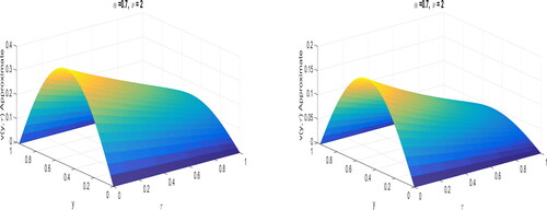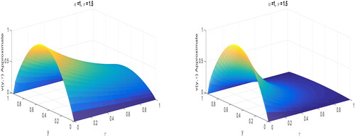The impact of fractional order in time for fixed $\nu =1.9$ and varying α is presented in Figure 2. It can be observed that the fractional order α and ν moulds the shape of the solutions. The influence of co-efficient $K_{\nu }$ on solution profile of (26(26) $${}^{\mathit{ABC}}{D}_{\tau }^{\alpha }v(y,\tau )=K_{\nu }\frac{{\partial }^{\nu }}{\partial |y{|}^{\nu }}v(y,\tau ),\hspace{1em}0<y<1,0<\tau <1,$$(26) ) for $\alpha =0.7, \nu =2$ and $\alpha =1, \nu =1.5$ can be viewed in Figures 3 and 4, respectively. This concludes that the dynamics of fractional diffusion equation also dependent on the diffusion coefficient.

Figure 1. Numerical solutions for $K_{\nu }=0.25, \tau =0.002, h=0.0314,\alpha =0.9$ and $\nu =1.2,1.7.$

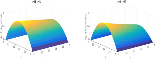
Figure 2. Numerical solutions for $K_{\nu }=0.25, \tau =0.002, h=0.0314,\nu =1.9$ and $\alpha =0.2,0.7.$

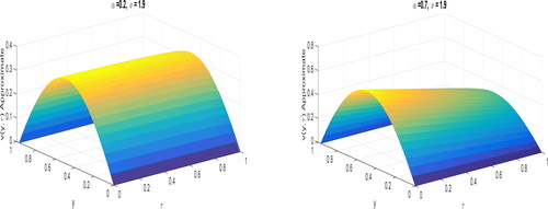
Figure 3. Effect of varying diffusion co-efficient $K_{\nu }$ for $\alpha =0.7, \nu =2, \tau =0.002, h=0.0314.$

6. Conclusion

In this article, we analysed the fractional diffusion equations by using the new fractional derivative recently introduced by Abdon Atangana and Dumitru Baleanu based on the Mittag-Leffler function involving non-singular and non-local kernels. The above mentioned aspects permit better description of the systems with memory that is dissipative and complex identically. The numerical scheme for solving the linear and non-linear time-space fractional diffusion equation governed by ABC fractional derivative of order. Primarily, we combined the trapezoidal formula for fractional integral approximation with a centered difference approximation of the Riesz fractional derivative with second-order accuracy in space to attain the numerical scheme for the linear time-space fractional diffusion equation. Afterwards, we have extended the scheme to get the solution of the non-linear time-space fractional diffusion equation. The stability of the proposed scheme has been established analytically. Also, we investigated the convergence of the proposed scheme and proved that the proposed scheme converges at the rate of $O(t^2+h^2)$ having space mesh size h and time step t. Numerical simulations are presented to demonstrate the effect of fractional order in space and time and the impact of varying the diffusion co-efficient $K_{\nu }$ on fractional diffusion equations in Figures 1–4.

Figure 4. Effect of varying diffusion co-efficient $K_{\nu }$ for $\alpha =1, \nu =1.5, \tau =0.002, h=0.0314.$

Disclosure statement

No potential conflict of interest was reported by the authors.

References

- Algahtani, O. J. J. (2016). Comparing the Atangana–Baleanu and Caputo–Fabrizio derivative with fractional order: Allen Cahn model. Chaos, Solitons and Fractals, 89, 552–559. doi:10.1016/j.chaos.2016.03.026
- Atangana, A., & Baleanu, D. (2016). New fractional derivatives with nonlocal and non-singular kernel: Theory and application to heat transfer model. Thermal Science, 20(2), 763–769. doi:10.2298/TSCI160111018A
- Bao, N. T., Baleanu, D., Minh, D. L. T., & Huy, T. N. (2020). Regularity results for fractional diffusion equations involving fractional derivative with Mittag–Leffler kernel. Mathematical Methods in the Applied Sciences, 43(12), 7208–7226. doi:10.1002/mma.6459
- Baleanu, D., Shiri, B., Srivastava, H. M., & Qurashi, M. A. (2018). A Chebyshev spectral method based on operational matrix for fractional differential equations involving non-singular Mittag-Leffler kernel. Advances in Difference Equations, 1, 1–23.
- Baskonus, H. M., & Bulut, H. (2016). Regarding on the prototype solutions for the nonlinear fractional-order biological population model. AIP Conference Proceedings, 1738(1), 1–5.
- Baskonus, H. M., Mekkaoui, T., Hammouch, Z., & Bulut, H. (2015). Active control of a chaotic fractional order economic system. Entropy, 17(12), 5771–5783. doi:10.3390/e17085771
- Celik, C., & Duman, M. (2012). Crank–Nicolson method for the fractional diffusion equation with the Riesz fractional derivative. Journal of Computational Physics, 231(4), 1743–1750. doi:10.1016/j.jcp.2011.11.008
- Dixon, J., & McKee, S. (1986). Weakly singular discrete Gronwall inequalities. ZAMM - Journal of Applied Mathematics and Mechanics/Zeitschrift Für Angewandte Mathematik Und Mechanik, 66(11), 535–544. doi:10.1002/zamm.19860661107
- Evirgen, F., & Özdemir, N. (2011). Multistage adomian decomposition method for solving NLP problems over a nonlinear fractional dynamical system. Journal of Computational and Nonlinear Dynamics, 6(2), 021003–021009.
- Henry, B. I., Langlands, T. A. M., & Straka, P. (2009). An Introduction to Fractional Diffusion. World Science Review, doi:10.1142/9789814277327_0002
- Huang, J., & Yang, D. (2017). A unified difference-spectral method for time-space fractional diffusion equations. International Journal of Computer Mathematics, 94(6), 1172–1184. doi:10.1080/00207160.2016.1184262
- Huang, J. F., Tang, Y. F., & Väzquez, L. (2012). Convergence analysis of a block-by-block method for fractional differential equations. Numerical Mathematics: Theory, Methods and Applications, 5(2), 229–241. doi:10.4208/nmtma.2012.m1038
- Jain, S., Nieto, J. J., Singh, G., & Choi, J. (2020). Certain generating relations involving the generalized multi-index Bessel–Maitland function. Mathematical Problems in Engineering, 2020, 1–5.
- Jajarmi, A., Arshad, S., & Baleanu, D. (2019). A new fractional modelling and control strategy for the outbreak of dengue fever. Physica A: Statistical Mechanics and Its Applications, 535, 122524. doi:10.1016/j.physa.2019.122524
- Kumar, S., & Pandey, P. (2020a). Quasi wavelet numerical approach of non-linear reaction diffusion and integro reaction-diffusion equation with Atangana–Baleanu time fractional derivative. Chaos, Solitons and Fractals, 130, 109456. doi:10.1016/j.chaos.2019.109456
- Kumar, S., & Pandey, P. (2020b). A Legendre spectral finite difference method for the solution of non-linear space-time fractional Burger’s–Huxley and reaction-diffusion equation with Atangana–Baleanu derivative. Chaos, Solitons and Fractals, 130, 109402. doi:10.1016/j.chaos.2019.109402
- Mainardi, F., Luchko, Y., & Pagnini, G. (2001). The fundamental solution of the space-time fractional diffusion equation. Fractional Calculus and Applied Analysis, 4(2), 153–192.
- Ortigueira, M. D. (2006). Riesz potential operators and inverses via fractional centred derivatives. International Journal of Mathematics and Mathematical Sciences, 2006, 1–12. doi:10.1155/IJMMS/2006/48391
- Rezapour, S., Etemad, S., Tellab, B., Agarwal, P., & Guirao, J. L. G. (2021). Numerical Solutions Caused by DGJIM and ADM methods for multi-term fractional BVP involving the generalized ψ-RL-operators. Symmetry, 13(4), 1–21.
- Salahshour, S., Ahmadian, A., Senu, N., Baleanu, D., & Agarwal, P. (2015). On analytical solutions of the fractional differential equation with uncertainty: application to the Basset problem. Entropy, 17(2), 885–902. doi:10.3390/e17020885
- Santos, M. D. (2018). Non-Gaussian distributions to random walk in the context of memory kernels. Fractal and Fractional, 2(3), 1–15.
- Santos, M. D. (2019). Fractional prabhakar derivative in diffusion equation with non-static stochastic resetting. Physics, 1(1), 40–58.
- Sene, N. (2018!). Stokes first problem for heated flat plate with Atangana Baleanu fractional derivative. Chaos, Solitons and Fractals, 117, 68–75. doi:10.1016/j.chaos.2018.10.014
- Sene, N., & Abdelmalek, K. (2019). Analysis of the fractional diffusion equations described by Atangana-Baleanu-Caputo fractional derivative. Chaos, Solitons and Fractals, 127, 158–164. doi:10.1016/j.chaos.2019.06.036
- Syam, M. I., & Al-Refai, M. (2019). Fractional differential equations with Atangana–Baleanu fractional derivative: analysis and applications. Chaos, Solitons and Fractals: X, 2, 100013. doi:10.1016/j.csfx.2019.100013
- Tajadodi, H. (2020). A Numerical approach of fractional advection-diffusion equation with Atangana–Baleanu derivative. Chaos, Solitons and Fractals, 130, 109527. doi:10.1016/j.chaos.2019.109527
- Yadav, S., Pandey, R. K., & Shukla, A. (2019). Numerical approximations of Atangana–Baleanu Caputo derivative and its application. Chaos, Solitons and Fractals, 118, 58–64. doi:10.1016/j.chaos.2018.11.009
- Yang, Q., Liu, F., & Turner, I. (2010). Numerical methods for fractional partial differential equations with Riesz space fractional derivatives. Applied Mathematical Modelling, 34(1), 200–218. doi:10.1016/j.apm.2009.04.006
- Zhou, S. S., Areshi, M., Agarwal, P., Shah, N. A., Chung, J. D., & Nonlaopon, K. (2021). Analytical analysis of fractional-order multi-dimensional dispersive partial differential equations. Symmetry, 13(6), 939–913. doi:10.3390/sym13060939