Incommensurate conformable-type three-dimensional Lotka–Volterra model: discretization, stability, and bifurcation

Abstract

The classic Lotka–Volterra model is a two-dimensional system of differential equations used to model population dynamics among two-species: a predator and its prey. In this article, we consider a modified three-dimensional fractional-order Lotka–Volterra system that models population dynamics among three-species: a predator, an omnivore and their mutual prey. Biologically speaking, population models with a discrete and continuous structure often provide richer dynamics than either discrete or continuous models, so we first discretize the model while keeping one time-continuous dependent variable in each equation. Then, we analyze the stability and bifurcation near the equilibria. The results demonstrated that the dynamic behaviors of the discretized model are sensitive to the fractional-order parameter and discretization parameter. Finally, numerical simulations are performed to explain and validate the findings, and the maximum Lyapunov exponents is computed to confirm the presence of chaotic behavior in the studied model.

Keywords:

• Conformable fractional derivative
• prey–predator– omnivore system
• discretization
• stability
• bifurcations
• chaos

1. Introduction

The dynamic behaviors studies of nonlinear models emerging in engineering and science play a considerable role in our daily activities. Population dynamics models are widely used in ecology. Understanding the dynamics of prey–predator interactions is one of the most primary operations that shape the framework and function of ecological societies (Rilov, 2009). For instance, some recent experimental studies have demonstrated that ocean acidification influence prey–predator interactions (Kroeker, Sanford, Jellison, & Gaylord, 2014) as ocean acidification makes it difficult for sea snails to burrow from their sea star predators (Jellison, Ninokawa, Hill, Sanford, & Gaylord, 2016). The oldest and most celebrated prey–predator model is the Lotka–Volterra model, independently introduced by Lotka (Lotka, 1925) and Volterra (Volterra, 1926). This model is formulated in ordinary differential equations such that any slight change of the model will lead to a qualitatively different type of behavior. The Lotka–Volterra model may indeed be the simplest possible prey–predator model. Nevertheless, it is a useful tool that contains the essential features of real ecosystems, and serves as a robust foundation from which it is possible to develop more sophisticated generalized models (Korobeinikov & Wake, 1999).

Recently, it has been shown that many mathematical models can be effectively reformulated via noninteger-order differential equations owing to the unsuitability and ability of the integer-order differential equations in modeling many phenomena (Yousef et al., 2019). The noninteger-order derivatives are oftentimes called fractional-order derivatives or artlessly fractional derivatives. It is well known that the derivatives with integer-order are in local nature, unlike the derivatives with fractional-order (Yousef et al., 2019). It has been evinced that the nonlocality merit of the fractional derivatives is employed to make them a suitable tool for describing the dynamic behaviours of many life phenomena and dynamical models that have inherited the properties of memory (Du, Wang, & Hu, 2013; Alquran, Yousef, Alquran, Sulaiman, & Yusuf, 2021). Consequently, many existing differential equations describing various phenomena in engineering and science have been recast by means of fractional derivatives (Gurcan, Kaya, & Kartal, 2019; Wang, Xie, Lu, & Li, 2019; Elsadany & Matouk, 2015; Ahmed & Elgazzar, 2007; Ahmed, El-Sayed, & El-Saka, 2007; Yousef, Semmar, & Al Nasr, 2022), and their solutions and dynamic behaviors continue to gain widespread attention today in many other disciplines (Abu Arqub, 2018; Yousef, Alkam, & Saker, 2020; Arqub, Osman, Abdel-Aty, Mohamed, & Momani, 2020; Djennadi, Shawagfeh, Osman, Gómez-Aguilar, & Arqub, 2021; Ali et al., 2020; Inan, Osman, Ak, & Baleanu, 2020; Kumar, Chauhan, Osman, & Mohiuddine, 2021; Kumar, Chauhan, et al., 2021; Jaradat et al., 2020; Jaradat, Alquran, Yousef, Momani, & Baleanu, 2019; Maayah, Yousef, Arqub, Momani, & Alsaedi, 2019; Momani, Arqub, Maayah, Yousef, & Alsaedi, 2018).

In an ecosystem, we may accept a three-species model that includes prey, predator, and omnivore. An omnivore is a predator that feeds on several trophic levels (Diethelm & Ford, 2002), and it has been seen in food chain models of three or more species. In the present work, we will consider an incommensurate conformable-type fractional-order prey–predator–omnivore model. It is noteworthy that the omnivore considered in the current work is presented as a top scavenger predator, which not only devours the corpses of the predator, but also predates the thoroughbred prey. The investigated system reads as: (1) $$\{\begin{array}{c}{D}_s^{\alpha }x(t)=rx(t)(1-x(t))-ax(t)y(t)-x(t)z(t),\hfill \\ D_s^{\beta }y(t)=y(t)(-c+dx(t)),\hfill \\ D_s^{\gamma }z(t)=x(t)z(t)-bz(t)+ey(t)z(t)-f{z}^2(t),\hfill \end{array}$$(1) where the conformable fractional derivative $D_s^{\tilde{\alpha }}$ is defined for a function $f:[s,\infty )\to \mathbb{R},s\ge 0,$ as (Khalil, Al Horani, Yousef, & Sababheh, 2014) (2) $$D_s^{\tilde{\alpha }}f(t)=\underset{ϵ\to 0}{\lim }\frac{f\left(t+ϵ{(t-s)}^{1-\tilde{\alpha }}\right)-f(t)}{ϵ},\hspace{1em}0<\tilde{\alpha }<1,$$(2) and all the constant coefficients $a,b,c,d,e,f$ and r are positive real numbers. In this model, the positive functions $x(t),y(t),$ and z(t) stand for the prey, predator and omnivore densities at time t, respectively.

From Equation (2)(2) $$D_s^{\tilde{\alpha }}f(t)=\underset{ϵ\to 0}{\lim }\frac{f\left(t+ϵ{(t-s)}^{1-\tilde{\alpha }}\right)-f(t)}{ϵ},\hspace{1em}0<\tilde{\alpha }<1,$$(2) , it has been evinced in (Abdeljawad, 2015) the following necessary fact (3) $$D_s^{\tilde{\alpha }}f(t)={(t-s)}^{1-\tilde{\alpha }}f\prime (t).$$(3)

2. Discretization process

Several studies revealed that the discrete-time system exhibits much fruitful dynamic behaviors, such as bifurcations and chaos, than those of its continuous-time system counterpart. Consequently, in this section, we aim to discretize the model (1)(1) $$\{\begin{array}{c}{D}_s^{\alpha }x(t)=rx(t)(1-x(t))-ax(t)y(t)-x(t)z(t),\hfill \\ D_s^{\beta }y(t)=y(t)(-c+dx(t)),\hfill \\ D_s^{\gamma }z(t)=x(t)z(t)-bz(t)+ey(t)z(t)-f{z}^2(t),\hfill \end{array}$$(1) making use of the piecewise-constant approximation (Kartal & Gurcan, 2019) as shown below. (4) $$\{\begin{array}{c}{D}_s^{\alpha }x(t)=rx(t)(1-x(t))-ax(t)y\left(\right[\frac{t}{h}\left]h\right)-x(t)z\left(\right[\frac{t}{h}\left]h\right),\hfill \\ D_s^{\beta }y(t)=y(t)(-c+dx(\left[\frac{t}{h}\right]h)),\hfill \\ D_s^{\gamma }z(t)=x\left(\right[\frac{t}{h}\left]h\right)z(t)-bz(t)+ey\left(\right[\frac{t}{h}\left]h\right)z(t)-f{z}^2(t),\hfill \end{array}$$(4) where $[\frac{t}{h}]$ denotes the integer part of $t\in [nh,(n+1)h),n=0,1,\dots ,$ and h > 0 is a discretization parameter.

Applying the rule in Equation (3)(3) $$D_s^{\tilde{\alpha }}f(t)={(t-s)}^{1-\tilde{\alpha }}f\prime (t).$$(3) to the first equation in the system (4)(4) $$\{\begin{array}{c}{D}_s^{\alpha }x(t)=rx(t)(1-x(t))-ax(t)y\left(\right[\frac{t}{h}\left]h\right)-x(t)z\left(\right[\frac{t}{h}\left]h\right),\hfill \\ D_s^{\beta }y(t)=y(t)(-c+dx(\left[\frac{t}{h}\right]h)),\hfill \\ D_s^{\gamma }z(t)=x\left(\right[\frac{t}{h}\left]h\right)z(t)-bz(t)+ey\left(\right[\frac{t}{h}\left]h\right)z(t)-f{z}^2(t),\hfill \end{array}$$(4) , gives the following Bernoulli differential equation: (5) $${(t-nh)}^{1-\alpha }\frac{dx(t)}{dt}+(z(nh)+ay(nh)-r)x(t)=-r{x}^2(t),$$(5) which leads to (6) $$-\frac{x\prime (t)}{x^2(t)}+\frac{(r-z(nh)-ay(nh))}{x(t){(t-nh)}^{1-\alpha }}=\frac{r}{{(t-nh)}^{1-\alpha }}.$$(6)

Next, multiply Equation (6)(6) $$-\frac{x\prime (t)}{x^2(t)}+\frac{(r-z(nh)-ay(nh))}{x(t){(t-nh)}^{1-\alpha }}=\frac{r}{{(t-nh)}^{1-\alpha }}.$$(6) by $e^{(r-z(nh)-ay(nh))\frac{{(t-nh)}^{\alpha }}{\alpha }},$ to obtain (7) $$\frac{d}{dt}\left(\frac{1}{x(t)}{e}^{(r-z(nh)-ay(nh))\frac{{(t-nh)}^{\alpha }}{\alpha }}\right)=\frac{r}{{(t-nh)}^{1-\alpha }}{e}^{(r-z(nh)-ay(nh))\frac{{(t-nh)}^{\alpha }}{\alpha }},t\in [nh,(n+1)h).$$(7)

Integrating Equation (7)(7) $$\frac{d}{dt}\left(\frac{1}{x(t)}{e}^{(r-z(nh)-ay(nh))\frac{{(t-nh)}^{\alpha }}{\alpha }}\right)=\frac{r}{{(t-nh)}^{1-\alpha }}{e}^{(r-z(nh)-ay(nh))\frac{{(t-nh)}^{\alpha }}{\alpha }},t\in [nh,(n+1)h).$$(7) on the interval $[nh,t),$ we get (8) $$\frac{1}{x(t)}{e}^{(r-z(nh)-ay(nh))\frac{{(t-nh)}^{\alpha }}{\alpha }}-\frac{1}{x(nh)}=\frac{r}{(r-z(nh)-ay(nh))}[e^{(r-z(nh)-ay(nh))\frac{{(t-nh)}^{\alpha }}{\alpha }}-1].$$(8)

Let $t\to (n+1)h$ in Equation (8)(8) $$\frac{1}{x(t)}{e}^{(r-z(nh)-ay(nh))\frac{{(t-nh)}^{\alpha }}{\alpha }}-\frac{1}{x(nh)}=\frac{r}{(r-z(nh)-ay(nh))}[e^{(r-z(nh)-ay(nh))\frac{{(t-nh)}^{\alpha }}{\alpha }}-1].$$(8) and replace x(nh) by x_n, yields (9) $$x_{n+1}=\frac{x_n(r-z_n-a{y}_n)}{r{x}_n+(r-z_n-a{y}_n-r{x}_n)e^{-(r-z_n-a{y}_n)\frac{h^{\alpha }}{\alpha }}}.$$(9)

On a similar manner, from the second equation in the system (4)(4) $$\{\begin{array}{c}{D}_s^{\alpha }x(t)=rx(t)(1-x(t))-ax(t)y\left(\right[\frac{t}{h}\left]h\right)-x(t)z\left(\right[\frac{t}{h}\left]h\right),\hfill \\ D_s^{\beta }y(t)=y(t)(-c+dx(\left[\frac{t}{h}\right]h)),\hfill \\ D_s^{\gamma }z(t)=x\left(\right[\frac{t}{h}\left]h\right)z(t)-bz(t)+ey\left(\right[\frac{t}{h}\left]h\right)z(t)-f{z}^2(t),\hfill \end{array}$$(4) , we have (10) $$\frac{dy(t)}{y(t)}=\frac{(dx(nh)-c)}{{(t-nh)}^{1-\beta }}dt.$$(10)

Integrating both sides of Equation (10)(10) $$\frac{dy(t)}{y(t)}=\frac{(dx(nh)-c)}{{(t-nh)}^{1-\beta }}dt.$$(10) on the interval $[nh,t),$ leads to (11) $$\text{ln}\hspace{0.17em}y(t)-\hspace{0.17em}\text{ln}\hspace{0.17em}y(nh)=(dx(nh)-c)\frac{{(t-nh)}^{\beta }}{\beta },t\in [nh,(n+1)h).$$(11)

For $t\to (n+1)h$ in Equation (11)(11) $$\text{ln}\hspace{0.17em}y(t)-\hspace{0.17em}\text{ln}\hspace{0.17em}y(nh)=(dx(nh)-c)\frac{{(t-nh)}^{\beta }}{\beta },t\in [nh,(n+1)h).$$(11) and replacing y(nh) with y_n, we obtain (12) $$y_{n+1}=y_n{e}^{(d{x}_n-c)\frac{h^{\beta }}{\beta }}.$$(12)

Again, similar to the first equation, we get (13) $$z_{n+1}=\frac{z_n(x_n+e{y}_n-b)}{f{z}_n+(x_n+e{y}_n-f{z}_n-b)e^{-(x_n+e{y}_n-b)\frac{h^{\gamma }}{\gamma }}}.$$(13)

As a consequence, the discrete version of the model (4)(4) $$\{\begin{array}{c}{D}_s^{\alpha }x(t)=rx(t)(1-x(t))-ax(t)y\left(\right[\frac{t}{h}\left]h\right)-x(t)z\left(\right[\frac{t}{h}\left]h\right),\hfill \\ D_s^{\beta }y(t)=y(t)(-c+dx(\left[\frac{t}{h}\right]h)),\hfill \\ D_s^{\gamma }z(t)=x\left(\right[\frac{t}{h}\left]h\right)z(t)-bz(t)+ey\left(\right[\frac{t}{h}\left]h\right)z(t)-f{z}^2(t),\hfill \end{array}$$(4) is given by the following difference equations: (14) $$\{\begin{array}{c}{x}_{n+1}=\frac{x_n(r-z_n-a{y}_n)}{r{x}_n+(r-z_n-a{y}_n-r{x}_n)e^{-(r-z_n-a{y}_n)\frac{h^{\alpha }}{\alpha }}},\hfill \\ y_{n+1}=y_n{e}^{(d{x}_n-c)\frac{h^{\beta }}{\beta }},\hfill \\ z_{n+1}=\frac{z_n(x_n+e{y}_n-b)}{f{z}_n+(x_n+e{y}_n-f{z}_n-b)e^{-(x_n+e{y}_n-b)\frac{h^{\gamma }}{\gamma }}}.\hfill \end{array}$$(14)

3. Equilibria and analysis of local stability

In this section, we explore the local stability for the system of difference Equation (14)(14) $$\{\begin{array}{c}{x}_{n+1}=\frac{x_n(r-z_n-a{y}_n)}{r{x}_n+(r-z_n-a{y}_n-r{x}_n)e^{-(r-z_n-a{y}_n)\frac{h^{\alpha }}{\alpha }}},\hfill \\ y_{n+1}=y_n{e}^{(d{x}_n-c)\frac{h^{\beta }}{\beta }},\hfill \\ z_{n+1}=\frac{z_n(x_n+e{y}_n-b)}{f{z}_n+(x_n+e{y}_n-f{z}_n-b)e^{-(x_n+e{y}_n-b)\frac{h^{\gamma }}{\gamma }}}.\hfill \end{array}$$(14) around selected equilibria. It is readily verified that the following points are from the equilibria of system (1)(1) $$\{\begin{array}{c}{D}_s^{\alpha }x(t)=rx(t)(1-x(t))-ax(t)y(t)-x(t)z(t),\hfill \\ D_s^{\beta }y(t)=y(t)(-c+dx(t)),\hfill \\ D_s^{\gamma }z(t)=x(t)z(t)-bz(t)+ey(t)z(t)-f{z}^2(t),\hfill \end{array}$$(1) :

The trivial state $E_0=(0,0,0),$ the axial state $E_1=(1,0,0),$ the boundary state $E_2=(\frac{c}{d},\frac{r(d-c)}{ad},0),$ and the coexistence state $E_3=(\frac{c}{d},\frac{d(b+rf)-c(1+rf)}{d(e+af)},\frac{a(c-bd)-re(c-d)}{d(e+af)}).$

Theorem 3.1.

The equilibrium $E_0=(0,0,0)$ of system (14) is a saddle point.

Proof.

The Jacobian matrix computed at the equilibrium E₀ is given as $$J(E_0)=\left(\begin{array}{ccc}{e}^{r\frac{h^{\alpha }}{\alpha }}& 0& 0\\ 0& e^{-c\frac{h^{\beta }}{\beta }}& 0\\ 0& 0& e^{-b\frac{h^{\gamma }}{\gamma }}\end{array}\right)$$ and has eigenvalues ${\lambda }_1=e^{r\frac{h^{\alpha }}{\alpha }},$ ${\lambda }_2=e^{-c\frac{h^{\beta }}{\beta }}$ and ${\lambda }_3=e^{-b\frac{h^{\gamma }}{\gamma }}.$ Thus, E₀ is a saddle point since $\left|{\lambda }_1\right|>1,\left|{\lambda }_2\right|<1$ and $\left|{\lambda }_3\right|<1.$ □

Theorem 3.2.

The equilibrium $E_1=(1,0,0)$ of system (14)(14) $$\{\begin{array}{c}{x}_{n+1}=\frac{x_n(r-z_n-a{y}_n)}{r{x}_n+(r-z_n-a{y}_n-r{x}_n)e^{-(r-z_n-a{y}_n)\frac{h^{\alpha }}{\alpha }}},\hfill \\ y_{n+1}=y_n{e}^{(d{x}_n-c)\frac{h^{\beta }}{\beta }},\hfill \\ z_{n+1}=\frac{z_n(x_n+e{y}_n-b)}{f{z}_n+(x_n+e{y}_n-f{z}_n-b)e^{-(x_n+e{y}_n-b)\frac{h^{\gamma }}{\gamma }}}.\hfill \end{array}$$(14) is a

1. saddle point if $d>c$ or $b<1$;

2. sink if $d<c$ and $b>1$;

3. non-hyperbolic if $d=c$ or $b=1.$

Proof.

The Jacobian matrix computed at the equilibrium E₁ of the linearization of system (14)(14) $$\{\begin{array}{c}{x}_{n+1}=\frac{x_n(r-z_n-a{y}_n)}{r{x}_n+(r-z_n-a{y}_n-r{x}_n)e^{-(r-z_n-a{y}_n)\frac{h^{\alpha }}{\alpha }}},\hfill \\ y_{n+1}=y_n{e}^{(d{x}_n-c)\frac{h^{\beta }}{\beta }},\hfill \\ z_{n+1}=\frac{z_n(x_n+e{y}_n-b)}{f{z}_n+(x_n+e{y}_n-f{z}_n-b)e^{-(x_n+e{y}_n-b)\frac{h^{\gamma }}{\gamma }}}.\hfill \end{array}$$(14) is given as $$J(E_1)=\left(\begin{array}{ccc}{e}^{-r\frac{h^{\alpha }}{\alpha }}& \frac{a}{r}(-1+e^{-r\frac{h^{\alpha }}{\alpha }})& \frac{1}{r}(-1+e^{-r\frac{h^{\alpha }}{\alpha }})\\ 0& e^{(-c+d)\frac{h^{\beta }}{\beta }}& 0\\ 0& 0& e^{(1-b)\frac{h^{\gamma }}{\gamma }}\end{array}\right)$$ and has eigenvalues ${\lambda }_1=e^{-r\frac{h^{\alpha }}{\alpha }},$ which satisfy $\left|{\lambda }_1\right|<1,{\lambda }_2=e^{(-c+d)\frac{h^{\beta }}{\beta }}$ and ${\lambda }_3=e^{(1-b)\frac{h^{\gamma }}{\gamma }}.$ Now, we consider the following cases:

1. if $d>c$ or $b<1,$ then $\left|{\lambda }_2\right|>1$ or $\left|{\lambda }_3\right|>1$ and E₁ is a saddle point;

2. if $d<c$ and $b>1,$ then $\left|{\lambda }_2\right|<1$ and $\left|{\lambda }_3\right|<1$ and E₁ is a sink;

3. if $d=c$ or $b=1,$ then $\left|{\lambda }_2\right|=1$ or $\left|{\lambda }_3\right|=1$ and E₁ is a non-hyperbolic.

Theorem 3.3.

The equilibrium $E_2=(\frac{c}{d},\frac{r(d-c)}{ad},0)$ is local asymptotically stable if $d<(c+\frac{\beta }{h^{\beta }})$ and $r<\frac{a(bd-c)}{e(d-c)}.$

Proof.

The Jacobian matrix for system (14)(14) $$\{\begin{array}{c}{x}_{n+1}=\frac{x_n(r-z_n-a{y}_n)}{r{x}_n+(r-z_n-a{y}_n-r{x}_n)e^{-(r-z_n-a{y}_n)\frac{h^{\alpha }}{\alpha }}},\hfill \\ y_{n+1}=y_n{e}^{(d{x}_n-c)\frac{h^{\beta }}{\beta }},\hfill \\ z_{n+1}=\frac{z_n(x_n+e{y}_n-b)}{f{z}_n+(x_n+e{y}_n-f{z}_n-b)e^{-(x_n+e{y}_n-b)\frac{h^{\gamma }}{\gamma }}}.\hfill \end{array}$$(14) computed at the equilibrium E₂ is given as $$J(E_2)=\left(\begin{array}{ccc}{e}^{-\frac{rc{h}^{\alpha }}{d\alpha }}& \frac{a}{r}(-1+e^{-\frac{rc{h}^{\alpha }}{d\alpha }})& \frac{1}{r}(-1+e^{-\frac{rc{h}^{\alpha }}{d\alpha }})\\ r(d-c)\frac{h^{\beta }}{a\beta }& 1& 0\\ 0& 0& e^{[\frac{c}{d}-b+\frac{er}{ad}(d-c)]\frac{h^{\gamma }}{\gamma }}\end{array}\right),$$ where the eigenvalues are ${\lambda }_1=e^{[\frac{c}{d}-b+\frac{er}{ad}(d-c)]\frac{h^{\gamma }}{\gamma }}$ and $${\lambda }_{2,3}=\frac{1}{2}(1+e^{-\frac{rc{h}^{\alpha }}{d\alpha }})\pm \frac{1}{2}{e}^{-\frac{rc{h}^{\alpha }}{d\alpha }}\sqrt{1-2e^{\frac{rc{h}^{\alpha }}{d\alpha }}+e^{2\frac{rc{h}^{\alpha }}{d\alpha }}+4e^{2\frac{rc{h}^{\alpha }}{d\alpha }}(-1+e^{-\frac{rc{h}^{\alpha }}{d\alpha }})(d-c)\frac{h^{\beta }}{\beta }}.$$

It’s effortless to check that ${\lambda }_{2,3}$ fulfill the equation ${\lambda }^2-\lambda Tr(M)+\mathit{Det}(M)=0,$ where (15) $$\begin{array}{c}M=\left(\begin{array}{cc}{e}^{-\frac{rc{h}^{\alpha }}{d\alpha }}& \frac{a}{r}(-1+e^{-\frac{rc{h}^{\alpha }}{d\alpha }})\\ r(d-c)\frac{h^{\beta }}{a\beta }& 1\end{array}\right),\\ Tr(M)=1+e^{-\frac{rc{h}^{\alpha }}{d\alpha }}\text{and\hspace{0.5em}Det}(M)=e^{-\frac{{\mathit{\text{rch}}}^{\alpha }}{d\alpha }}+\frac{h^{\beta }}{\beta }(d-c)\left({1-e}^{-\frac{{\mathit{\text{rch}}}^{\alpha }}{d\alpha }}\right).\end{array}$$(15)

Now, $\left|{\lambda }_1\right|<1$ whenever $r<\frac{a(bd-c)}{e(d-c)},$ and according to the Jury conditions (Kot, 2001), $\left|{\lambda }_{2,3}\right|<1$ whenever $d<(c+\frac{\beta }{h^{\beta }}).$ □

Theorem 3.4.

The positive equilibrium $E_3=(\frac{c}{d},\frac{d(b+rf)-c(1+rf)}{d(e+af)},\frac{a(c-bd)-re(c-d)}{d(e+af)})$ of system (14)(14) $$\{\begin{array}{c}{x}_{n+1}=\frac{x_n(r-z_n-a{y}_n)}{r{x}_n+(r-z_n-a{y}_n-r{x}_n)e^{-(r-z_n-a{y}_n)\frac{h^{\alpha }}{\alpha }}},\hfill \\ y_{n+1}=y_n{e}^{(d{x}_n-c)\frac{h^{\beta }}{\beta }},\hfill \\ z_{n+1}=\frac{z_n(x_n+e{y}_n-b)}{f{z}_n+(x_n+e{y}_n-f{z}_n-b)e^{-(x_n+e{y}_n-b)\frac{h^{\gamma }}{\gamma }}}.\hfill \end{array}$$(14) is local asymptotically stable if these inequalities are satisfied$$|C_1+C_3|<1+C_2,|C_1-3C_3|<3-C_2,\mathit{\text{and}}{\mathrm{C}}_3^2{+\mathrm{C}}_2{-\mathrm{C}}_1{\mathrm{C}}_3<1,$$where$$C_1=-1-e^{-\frac{rc{h}^{\alpha }}{d\alpha }}-e^{-[a(c-bd)+re(d-c)]\frac{f{h}^{\gamma }}{d\gamma (e+af)}},C_2=e^{-\frac{rc{h}^{\alpha }}{d\alpha }}+e^{-[a(c-bd)+re(d-c)]\frac{f{h}^{\gamma }}{d\gamma (e+af)}}(1+e^{-\frac{rc{h}^{\alpha }}{d\alpha }})+\frac{a{h}^{\beta }}{r\beta (e+af)}(1-e^{-\frac{rc{h}^{\alpha }}{d\alpha }})[d(b+rf)-c(1+rf)]+\frac{1}{fr}(1-e^{-\frac{rc{h}^{\alpha }}{d\alpha }})(1-e^{-[a(c-bd)+re(d-c)]\frac{f{h}^{\gamma }}{d\gamma (e+af)}}),$$and(16) $$\begin{array}{c}{C}_3=-e^{-[a(c-bd)+re(d-c)]\frac{f{h}^{\gamma }}{d\gamma (e+af)}}(e^{-\frac{rc{h}^{\alpha }}{d\alpha }}+\frac{a{h}^{\beta }}{r\beta (e+af)}(1-e^{-\frac{rc{h}^{\alpha }}{d\alpha }}\left)\right[d(b+rf)-c(1+rf)])\\ +\frac{1}{rf}(1-e^{-\frac{rc{h}^{\alpha }}{d\alpha }})(1-e^{-[a(c-bd)+re(d-c)]\frac{f{h}^{\gamma }}{d\gamma (e+af)}})[\frac{e{h}^{\beta }}{\beta (e+af)}(d(b+rf)-c(1+rf))-1].\end{array}$$(16)

Proof.

The Jacobian matrix for system (14)(14) $$\{\begin{array}{c}{x}_{n+1}=\frac{x_n(r-z_n-a{y}_n)}{r{x}_n+(r-z_n-a{y}_n-r{x}_n)e^{-(r-z_n-a{y}_n)\frac{h^{\alpha }}{\alpha }}},\hfill \\ y_{n+1}=y_n{e}^{(d{x}_n-c)\frac{h^{\beta }}{\beta }},\hfill \\ z_{n+1}=\frac{z_n(x_n+e{y}_n-b)}{f{z}_n+(x_n+e{y}_n-f{z}_n-b)e^{-(x_n+e{y}_n-b)\frac{h^{\gamma }}{\gamma }}}.\hfill \end{array}$$(14) computed at the equilibrium E₃ is given as $$J(E_3)=\left(\begin{array}{ccc}{e}^{-\frac{rc{h}^{\alpha }}{d\alpha }}& \frac{a}{r}(-1+e^{-\frac{rc{h}^{\alpha }}{d\alpha }})& \frac{1}{r}(-1+e^{-\frac{rc{h}^{\alpha }}{d\alpha }})\\ \frac{h^{\beta }}{\beta (e+af)}[d(b+rf)-c(1+rf)]& 1& 0\\ \frac{1}{f}(1-e^{-[a(c-bd)+re(d-c)]\frac{f{h}^{\gamma }}{d\gamma (e+af)}})& \frac{e}{f}(1-e^{-[a(c-bd)+re(d-c)]\frac{f{h}^{\gamma }}{d\gamma (e+af)}})& e^{-[a(c-bd)+re(d-c)]\frac{f{h}^{\gamma }}{d\gamma (e+af)}}\end{array}\right).$$

The characteristic polynomial for the above-mentioned Jacobian matrix is derived as: (17) $$P(\lambda )={\lambda }^3+C_1{\lambda }^2+C_2\lambda +C_3,$$(17) where the values of $C_1,C_2,$ and C₃ are as given in the Equation (16)(16) $$\begin{array}{c}{C}_3=-e^{-[a(c-bd)+re(d-c)]\frac{f{h}^{\gamma }}{d\gamma (e+af)}}(e^{-\frac{rc{h}^{\alpha }}{d\alpha }}+\frac{a{h}^{\beta }}{r\beta (e+af)}(1-e^{-\frac{rc{h}^{\alpha }}{d\alpha }}\left)\right[d(b+rf)-c(1+rf)])\\ +\frac{1}{rf}(1-e^{-\frac{rc{h}^{\alpha }}{d\alpha }})(1-e^{-[a(c-bd)+re(d-c)]\frac{f{h}^{\gamma }}{d\gamma (e+af)}})[\frac{e{h}^{\beta }}{\beta (e+af)}(d(b+rf)-c(1+rf))-1].\end{array}$$(16) .

Now, according to the Jury conditions (Grove & Ladas, 2004), the positive equilibrium E₃ of system (14)(14) $$\{\begin{array}{c}{x}_{n+1}=\frac{x_n(r-z_n-a{y}_n)}{r{x}_n+(r-z_n-a{y}_n-r{x}_n)e^{-(r-z_n-a{y}_n)\frac{h^{\alpha }}{\alpha }}},\hfill \\ y_{n+1}=y_n{e}^{(d{x}_n-c)\frac{h^{\beta }}{\beta }},\hfill \\ z_{n+1}=\frac{z_n(x_n+e{y}_n-b)}{f{z}_n+(x_n+e{y}_n-f{z}_n-b)e^{-(x_n+e{y}_n-b)\frac{h^{\gamma }}{\gamma }}}.\hfill \end{array}$$(14) is locally asymptotically stable if following conditions are hold: $|C_1+C_3|<1+C_2,|C_1-3C_3|<3-C_2$ and $C_3^2+C_2-C_1{C}_3<1.$ □

4. Neimark–Sacker bifurcation analysis

In this section, we investigate the presence of Neimark–Sacker bifurcation at the positive equilibria E₂ and E₃ of the discrete system (14)(14) $$\{\begin{array}{c}{x}_{n+1}=\frac{x_n(r-z_n-a{y}_n)}{r{x}_n+(r-z_n-a{y}_n-r{x}_n)e^{-(r-z_n-a{y}_n)\frac{h^{\alpha }}{\alpha }}},\hfill \\ y_{n+1}=y_n{e}^{(d{x}_n-c)\frac{h^{\beta }}{\beta }},\hfill \\ z_{n+1}=\frac{z_n(x_n+e{y}_n-b)}{f{z}_n+(x_n+e{y}_n-f{z}_n-b)e^{-(x_n+e{y}_n-b)\frac{h^{\gamma }}{\gamma }}}.\hfill \end{array}$$(14) .

Theorem 4.1.

The positive equilibrium point $E_2=(\frac{c}{d},\frac{r(d-c)}{ad},0)$ loses its stability via a Neimark–Sacker bifurcation when $d=c+\frac{\beta }{h^{\beta }}.$

Proof.

From Equation (15)(15) $$\begin{array}{c}M=\left(\begin{array}{cc}{e}^{-\frac{rc{h}^{\alpha }}{d\alpha }}& \frac{a}{r}(-1+e^{-\frac{rc{h}^{\alpha }}{d\alpha }})\\ r(d-c)\frac{h^{\beta }}{a\beta }& 1\end{array}\right),\\ Tr(M)=1+e^{-\frac{rc{h}^{\alpha }}{d\alpha }}\text{and\hspace{0.5em}Det}(M)=e^{-\frac{{\mathit{\text{rch}}}^{\alpha }}{d\alpha }}+\frac{h^{\beta }}{\beta }(d-c)\left({1-e}^{-\frac{{\mathit{\text{rch}}}^{\alpha }}{d\alpha }}\right).\end{array}$$(15) , we have Det(M) = 1 when $d=c+\frac{\beta }{h^{\beta }}.$ Hence, the equilibrium E₂ loses its stability via a Neimark–Sacker bifurcation when $d=c+\frac{\beta }{h^{\beta }}.$ □

Theorem 4.2.

The positive equilibrium $E_3=(\frac{c}{d},\frac{d(b+rf)-c(1+rf)}{d(e+af)},\frac{a(c-bd)-re(c-d)}{d(e+af)})$ of system (14)(14) $$\{\begin{array}{c}{x}_{n+1}=\frac{x_n(r-z_n-a{y}_n)}{r{x}_n+(r-z_n-a{y}_n-r{x}_n)e^{-(r-z_n-a{y}_n)\frac{h^{\alpha }}{\alpha }}},\hfill \\ y_{n+1}=y_n{e}^{(d{x}_n-c)\frac{h^{\beta }}{\beta }},\hfill \\ z_{n+1}=\frac{z_n(x_n+e{y}_n-b)}{f{z}_n+(x_n+e{y}_n-f{z}_n-b)e^{-(x_n+e{y}_n-b)\frac{h^{\gamma }}{\gamma }}}.\hfill \end{array}$$(14) undergoes a Neimark–Sacker bifurcation for $d(b+rf)>c(1+rf)$ and $a(c-bd)>re(c-d)$ if the following conditions are satisfied:$$1-C_2+C_3(C_1-C_3)=0,1+C_2-C_3(C_1+C_3)>0,1+C_1+C_2+C_3>0\text{and}{1-\mathrm{C}}_1{+\mathrm{C}}_2{-\mathrm{C}}_3>0,$$where the values of $C_1,C_2,$ and C₃ are as given in the Equation (16)(16) $$\begin{array}{c}{C}_3=-e^{-[a(c-bd)+re(d-c)]\frac{f{h}^{\gamma }}{d\gamma (e+af)}}(e^{-\frac{rc{h}^{\alpha }}{d\alpha }}+\frac{a{h}^{\beta }}{r\beta (e+af)}(1-e^{-\frac{rc{h}^{\alpha }}{d\alpha }}\left)\right[d(b+rf)-c(1+rf)])\\ +\frac{1}{rf}(1-e^{-\frac{rc{h}^{\alpha }}{d\alpha }})(1-e^{-[a(c-bd)+re(d-c)]\frac{f{h}^{\gamma }}{d\gamma (e+af)}})[\frac{e{h}^{\beta }}{\beta (e+af)}(d(b+rf)-c(1+rf))-1].\end{array}$$(16) .

Proof.

The characteristic polynomial for the Jacobian matrix of system (14)(14) $$\{\begin{array}{c}{x}_{n+1}=\frac{x_n(r-z_n-a{y}_n)}{r{x}_n+(r-z_n-a{y}_n-r{x}_n)e^{-(r-z_n-a{y}_n)\frac{h^{\alpha }}{\alpha }}},\hfill \\ y_{n+1}=y_n{e}^{(d{x}_n-c)\frac{h^{\beta }}{\beta }},\hfill \\ z_{n+1}=\frac{z_n(x_n+e{y}_n-b)}{f{z}_n+(x_n+e{y}_n-f{z}_n-b)e^{-(x_n+e{y}_n-b)\frac{h^{\gamma }}{\gamma }}}.\hfill \end{array}$$(14) computed at the equilibrium E₃ is given in Equation (17)(17) $$P(\lambda )={\lambda }^3+C_1{\lambda }^2+C_2\lambda +C_3,$$(17) . According to Lemma 4.1 in (Ali, Saeed, & Din, 2019) for n = 3, the positive equilibrium E₃ of system (14) undergoes a Neimark–Sacker bifurcation if the above-mentioned conditions are satisfied. □

5. Numerical simulations

Here, we aim to validate the above theoretical findings through numerical simulations where the numerical computations have been accomplished through the use of MATLAB-R2020a software. Let $a=0.61,b=0.197,c=0.16,d=0.93,e=0.651,f=0.673,h=0.75$ and $r=1,$ subject to the initial condition $(x(0),y(0),z(0))=(0.1,0.2,0.3).$ Figure 1 demonstrates the stable dynamic behaviors of the three-dimensional discrete system (14)(14) $$\{\begin{array}{c}{x}_{n+1}=\frac{x_n(r-z_n-a{y}_n)}{r{x}_n+(r-z_n-a{y}_n-r{x}_n)e^{-(r-z_n-a{y}_n)\frac{h^{\alpha }}{\alpha }}},\hfill \\ y_{n+1}=y_n{e}^{(d{x}_n-c)\frac{h^{\beta }}{\beta }},\hfill \\ z_{n+1}=\frac{z_n(x_n+e{y}_n-b)}{f{z}_n+(x_n+e{y}_n-f{z}_n-b)e^{-(x_n+e{y}_n-b)\frac{h^{\gamma }}{\gamma }}}.\hfill \end{array}$$(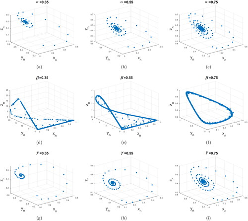14) , at the positive equilibrium E₃ by increasing one of the fractional-order parameters and fixing the other two. Note that if we increase the value of the fractional-order parameter α (taking α approaches one) with β and γ values fixed at 0.95, or if we increase the value of the fractional-order parameter γ (taking γ approaches one) with α and β values fixed at 0.95, then the discrete system (14)(14) $$\{\begin{array}{c}{x}_{n+1}=\frac{x_n(r-z_n-a{y}_n)}{r{x}_n+(r-z_n-a{y}_n-r{x}_n)e^{-(r-z_n-a{y}_n)\frac{h^{\alpha }}{\alpha }}},\hfill \\ y_{n+1}=y_n{e}^{(d{x}_n-c)\frac{h^{\beta }}{\beta }},\hfill \\ z_{n+1}=\frac{z_n(x_n+e{y}_n-b)}{f{z}_n+(x_n+e{y}_n-f{z}_n-b)e^{-(x_n+e{y}_n-b)\frac{h^{\gamma }}{\gamma }}}.\hfill \end{array}$$(14) going to stabilized. Whereas, increasing the value of the fractional-order parameter β with α and γ values fixed at 0.95, then chaotic behavior occurs.

Figure 1. Stable dynamical behavior of system (14)(14) $$\{\begin{array}{c}{x}_{n+1}=\frac{x_n(r-z_n-a{y}_n)}{r{x}_n+(r-z_n-a{y}_n-r{x}_n)e^{-(r-z_n-a{y}_n)\frac{h^{\alpha }}{\alpha }}},\hfill \\ y_{n+1}=y_n{e}^{(d{x}_n-c)\frac{h^{\beta }}{\beta }},\hfill \\ z_{n+1}=\frac{z_n(x_n+e{y}_n-b)}{f{z}_n+(x_n+e{y}_n-f{z}_n-b)e^{-(x_n+e{y}_n-b)\frac{h^{\gamma }}{\gamma }}}.\hfill \end{array}$$(14) subject to the initial condition $(x(0),y(0),z(0))=(0.1,0.2,0.3)$ for the parameters $a=0.61,b=0.197,c=0.16,d=0.93,e=0.651,f=0.673,h=0.75,$ and r = 1: (a)-(c) $\beta =\gamma =0.95,$ (d)-(f) $\alpha =\gamma =0.95,$ (g)-(i) $\alpha =\beta =0.95.$

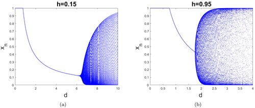
The bifurcation diagrams in Figure 2 show that with increasing value of the discretization parameter h with α, β and γ values fixed at 0.95 leads to destabilize the equilibrium E₂ through a Neimark–Sacker bifurcation.

Figure 2. Bifurcation diagram for the discrete system (14)(14) $$\{\begin{array}{c}{x}_{n+1}=\frac{x_n(r-z_n-a{y}_n)}{r{x}_n+(r-z_n-a{y}_n-r{x}_n)e^{-(r-z_n-a{y}_n)\frac{h^{\alpha }}{\alpha }}},\hfill \\ y_{n+1}=y_n{e}^{(d{x}_n-c)\frac{h^{\beta }}{\beta }},\hfill \\ z_{n+1}=\frac{z_n(x_n+e{y}_n-b)}{f{z}_n+(x_n+e{y}_n-f{z}_n-b)e^{-(x_n+e{y}_n-b)\frac{h^{\gamma }}{\gamma }}}.\hfill \end{array}$$(14) as a function of d for the parameters $a=1.5,b=2,c=0.75,e=0.951,f=0.89,r=1$ and $\alpha =0.95:$ (a) h = 0.15 and (b) h = 0.95.

Next, we examined the bifurcation and limit cycle for the system (14)(14) $$\{\begin{array}{c}{x}_{n+1}=\frac{x_n(r-z_n-a{y}_n)}{r{x}_n+(r-z_n-a{y}_n-r{x}_n)e^{-(r-z_n-a{y}_n)\frac{h^{\alpha }}{\alpha }}},\hfill \\ y_{n+1}=y_n{e}^{(d{x}_n-c)\frac{h^{\beta }}{\beta }},\hfill \\ z_{n+1}=\frac{z_n(x_n+e{y}_n-b)}{f{z}_n+(x_n+e{y}_n-f{z}_n-b)e^{-(x_n+e{y}_n-b)\frac{h^{\gamma }}{\gamma }}}.\hfill \end{array}$$(14) at the coexistence state E₃, choosing r as a bifurcation parameter. Figure 3 demonstrates that E₃ of system (14)(14) $$\{\begin{array}{c}{x}_{n+1}=\frac{x_n(r-z_n-a{y}_n)}{r{x}_n+(r-z_n-a{y}_n-r{x}_n)e^{-(r-z_n-a{y}_n)\frac{h^{\alpha }}{\alpha }}},\hfill \\ y_{n+1}=y_n{e}^{(d{x}_n-c)\frac{h^{\beta }}{\beta }},\hfill \\ z_{n+1}=\frac{z_n(x_n+e{y}_n-b)}{f{z}_n+(x_n+e{y}_n-f{z}_n-b)e^{-(x_n+e{y}_n-b)\frac{h^{\gamma }}{\gamma }}}.\hfill \end{array}$$(14) is stable for r < 0.275 and loses its stability thought a Neimark–Sacker bifurcation when r = 0.275 and an invariant circle appears for $0.275<r<0.595.$ Thereafter, for $r>0.595$ 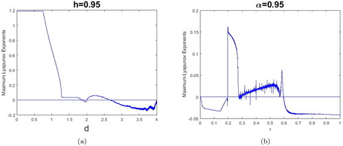the discrete system (14) return to stabilize. The maximum Lyapunov exponents corresponding to Figures 2(b) and 3(b) are given in Figure 4.

Figure 3. (a) Period-1 limit cycle for the discrete system (14)(14) $$\{\begin{array}{c}{x}_{n+1}=\frac{x_n(r-z_n-a{y}_n)}{r{x}_n+(r-z_n-a{y}_n-r{x}_n)e^{-(r-z_n-a{y}_n)\frac{h^{\alpha }}{\alpha }}},\hfill \\ y_{n+1}=y_n{e}^{(d{x}_n-c)\frac{h^{\beta }}{\beta }},\hfill \\ z_{n+1}=\frac{z_n(x_n+e{y}_n-b)}{f{z}_n+(x_n+e{y}_n-f{z}_n-b)e^{-(x_n+e{y}_n-b)\frac{h^{\gamma }}{\gamma }}}.\hfill \end{array}$$(14) by adopting the parameter values $a=0.61,b=0.397,c=0.16,e=0.651,f=0.17,d=0.673$ and $\alpha =0.95.$ (b) Bifurcation diagram of period-1 limit cycle of system (14)(14) $$\{\begin{array}{c}{x}_{n+1}=\frac{x_n(r-z_n-a{y}_n)}{r{x}_n+(r-z_n-a{y}_n-r{x}_n)e^{-(r-z_n-a{y}_n)\frac{h^{\alpha }}{\alpha }}},\hfill \\ y_{n+1}=y_n{e}^{(d{x}_n-c)\frac{h^{\beta }}{\beta }},\hfill \\ z_{n+1}=\frac{z_n(x_n+e{y}_n-b)}{f{z}_n+(x_n+e{y}_n-f{z}_n-b)e^{-(x_n+e{y}_n-b)\frac{h^{\gamma }}{\gamma }}}.\hfill \end{array}$$(14) .

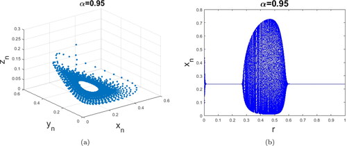
Figure 4. Maximum Lyapunov exponents corresponding to: (a) Fig. 2(b) and (b) Fig. 3(b).

6. Results and discussion

In this article, the dynamics of the incommensurate conformable-type fractional-order Lotka–Volterra model with omnivore are investigated. We have shown that the fractional-order parameters α, β and γ have impact on the stability of the discrete system. Chaos in the discrete system is studied. It is found that the system exhibits chaotic behavior when increasing β with fixing the fractional-order parameters α and γ. The simulation results displayed that the discretization parameter h is a key factor that affects dynamic behavior and is only responsible for a Neimark–Sacker bifurcation and chaos in the dynamic of the system (14)(14) $$\{\begin{array}{c}{x}_{n+1}=\frac{x_n(r-z_n-a{y}_n)}{r{x}_n+(r-z_n-a{y}_n-r{x}_n)e^{-(r-z_n-a{y}_n)\frac{h^{\alpha }}{\alpha }}},\hfill \\ y_{n+1}=y_n{e}^{(d{x}_n-c)\frac{h^{\beta }}{\beta }},\hfill \\ z_{n+1}=\frac{z_n(x_n+e{y}_n-b)}{f{z}_n+(x_n+e{y}_n-f{z}_n-b)e^{-(x_n+e{y}_n-b)\frac{h^{\gamma }}{\gamma }}}.\hfill \end{array}$$(14) . 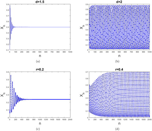When increasing the discretization parameter h with fixing the fractional-order parameters $\alpha ,\beta$ and γ, the discrete conformable-type system is destabilized and chaotic behavior occurs. In the analysis, d and r were chosen as bifurcation parameters for the equilibria E₂ and E₃, respectively. The results exhibited that the equilibrium E₃ possesses two Neimark–Sacker bifurcation points. To further confirm the chaos, we plot the time series of the system (14)(14) $$\{\begin{array}{c}{x}_{n+1}=\frac{x_n(r-z_n-a{y}_n)}{r{x}_n+(r-z_n-a{y}_n-r{x}_n)e^{-(r-z_n-a{y}_n)\frac{h^{\alpha }}{\alpha }}},\hfill \\ y_{n+1}=y_n{e}^{(d{x}_n-c)\frac{h^{\beta }}{\beta }},\hfill \\ z_{n+1}=\frac{z_n(x_n+e{y}_n-b)}{f{z}_n+(x_n+e{y}_n-f{z}_n-b)e^{-(x_n+e{y}_n-b)\frac{h^{\gamma }}{\gamma }}}.\hfill \end{array}$$(14) , see Figure 5. It is clear that when the bifurcation parameters d and r are increasing, this leads to chaotic behaviour in the system (14)(14) $$\{\begin{array}{c}{x}_{n+1}=\frac{x_n(r-z_n-a{y}_n)}{r{x}_n+(r-z_n-a{y}_n-r{x}_n)e^{-(r-z_n-a{y}_n)\frac{h^{\alpha }}{\alpha }}},\hfill \\ y_{n+1}=y_n{e}^{(d{x}_n-c)\frac{h^{\beta }}{\beta }},\hfill \\ z_{n+1}=\frac{z_n(x_n+e{y}_n-b)}{f{z}_n+(x_n+e{y}_n-f{z}_n-b)e^{-(x_n+e{y}_n-b)\frac{h^{\gamma }}{\gamma }}}.\hfill \end{array}$$(14) .

Figure 5. Time series plot of system (14)(14) $$\{\begin{array}{c}{x}_{n+1}=\frac{x_n(r-z_n-a{y}_n)}{r{x}_n+(r-z_n-a{y}_n-r{x}_n)e^{-(r-z_n-a{y}_n)\frac{h^{\alpha }}{\alpha }}},\hfill \\ y_{n+1}=y_n{e}^{(d{x}_n-c)\frac{h^{\beta }}{\beta }},\hfill \\ z_{n+1}=\frac{z_n(x_n+e{y}_n-b)}{f{z}_n+(x_n+e{y}_n-f{z}_n-b)e^{-(x_n+e{y}_n-b)\frac{h^{\gamma }}{\gamma }}}.\hfill \end{array}$$(14) with respect to Fig. 2(b) and Fig. 3(b): (a) Asymptotically stable for d = 1.5; (b) Chaotic for d = 2; (c) Asymptotically stable for r = 0.2; and (d) Chaotic for r = 0.4.

Disclosure statement

No potential conflict of interest was reported by the authors.

References

- Abdeljawad, T. (2015). On conformable fractional calculus. Journal of Computational and Applied Mathematics, 279, 57–66. doi:10.1016/j.cam.2014.10.016
- Abu Arqub, O. (2018). Numerical solutions of systems of first-order, two-point BVPs based on the reproducing kernel algorithm. Calcolo, 55(3), 1–28. doi:10.1007/s10092-018-0274-3
- Ahmed, E., & Elgazzar, A. S. (2007). On fractional order differential equations model for nonlocal epidemics. Physica A, 379(2), 607–614. doi:10.1016/j.physa.2007.01.010
- Ahmed, E., El-Sayed, A., & El-Saka, H. (2007). Equilibrium points, stability and numerical solutions of fractional-order predator–prey and rabies models. Journal of Mathematical Analysis and Applications, 325(1), 542–553. doi:10.1016/j.jmaa.2006.01.087
- Ali, I., Saeed, U., & Din, Q. (2019). Bifurcation analysis and chaos control in discrete-time system of three competing species. Arabian Journal of Mathematics, 8(1), 1–14. doi:10.1007/s40065-018-0207-7
- Ali, K. K., Abd El Salam, M. A., Mohamed, E. M., Samet, B., Kumar, S., & Osman, M. S. (2020). Numerical solution for generalized nonlinear fractional integro-differential equations with linear functional arguments using Chebyshev series. Advances in Continuous and Discrete Models, 2020, 1–23.
- Alquran, M., Yousef, F., Alquran, F., Sulaiman, T. A., & Yusuf, A. (2021). Dual-wave solutions for the quadratic-cubic conformable-Caputo time-fractional Klein-Fock-Gordon equation. Mathematics and Computers in Simulation, 185, 62–76. doi:10.1016/j.matcom.2020.12.014
- Arqub, O. A., Osman, M. S., Abdel-Aty, A. H., Mohamed, A., & Momani, S. (2020). A numerical algorithm for the solutions of ABC singular Lane–Emden type models arising in astrophysics using reproducing kernel discretization method. Mathematics, 8(6), 923. doi:10.3390/math8060923
- Diethelm, K., & Ford, N. J. (2002). Analysis of fractional differential equations. Journal of Mathematical Analysis and Applications, 265(2), 229–248. doi:10.1006/jmaa.2000.7194
- Djennadi, S., Shawagfeh, N., Osman, M. S., Gómez-Aguilar, J. F., & Arqub, O. A. (2021). The Tikhonov regularization method for the inverse source problem of time fractional heat equation in the view of ABC-fractional technique. Physica Scripta, 96(9):094006.
- Du, M., Wang, Z., & Hu, H. (2013). Measuring memory with the order of fractional derivative. Scientific Reports, 3(1), 1–3.
- Elsadany, A. A., & Matouk, A. E. (2015). Dynamical behaviors of fractional-order Lotka–Volterra predator–prey model and its discretization. Journal of Applied Mathematics and Computing, 49(1-2), 269–283. doi:10.1007/s12190-014-0838-6
- Grove, E. A., & Ladas, G. (2004). Periodicities in nonlinear difference equations (Vol. 4). Boca Raton: CRC Press.
- Gurcan, F., Kaya, G., & Kartal, S. (2019). Conformable fractional order lotka–volterra predator–prey model: Discretization, stability and bifurcation. J. Comput. Nonlinear Dynam, 14(11), 111007. doi:10.1115/1.4044313
- Inan, B., Osman, M. S., Ak, T., & Baleanu, D. (2020). Analytical and numerical solutions of mathematical biology models: The Newell–Whitehead–Segel and Allen-Cahn equations. Mathematical Methods in the Applied Sciences, 43(5), 2588–2600. doi:10.1002/mma.6067
- Jaradat, I., Alquran, M., Katatbeh, Q., Yousef, F., Momani, S., & Baleanu, D. (2020). An avant-garde handling of temporal-spatial fractional physical models. International Journal of Nonlinear Sciences and Numerical Simulation, 21(2), 183–194. doi:10.1515/ijnsns-2018-0363
- Jaradat, I., Alquran, M., Yousef, F., Momani, S., & Baleanu, D. 2019). On (2+1)-dimensional physical models endowed with decoupled spatial and temporal memory indices. The European Physical Journal plus, 134(7), 360. doi:10.1140/epjp/i2019-12769-8
- Jellison, B. M., Ninokawa, A. T., Hill, T. M., Sanford, E., & Gaylord, B. (2016). Ocean acidification alters the response of intertidal snails to a key sea star predator. Proceedings of the Royal Society B: Biological Sciences, 283(1833), 20160890. doi:10.1098/rspb.2016.0890
- Kartal, S., & Gurcan, F. (2019). Discretization of conformable fractional differential equations by a piecewise constant approximation. International Journal of Computer Mathematics, 96(9), 1849–1860. doi:10.1080/00207160.2018.1536782
- Khalil, R., Al Horani, M., Yousef, A., & Sababheh, M. (2014). A new definition of fractional derivative. Journal of Computational and Applied Mathematics, 264, 65–70. doi:10.1016/j.cam.2014.01.002
- Korobeinikov, A., & Wake, G. C. (1999). Global properties of the three-dimensional predator–prey Lotka–Volterra systems. Journal of Applied Mathematics Decision Sciences, 3(2), 155–162. doi:10.1155/S1173912699000085
- Kot, M. (2001). Elements of mathematical ecology. Cambridge: Cambridge University Press.
- Kroeker, K. J., Sanford, E., Jellison, B. M., & Gaylord, B. (2014). Predicting the effects of ocean acidification on predator-prey interactions: A conceptual framework based on coastal molluscs. The Biological Bulletin, 226(3), 211–222. doi:10.1086/BBLv226n3p211
- Kumar, S., Chauhan, R. P., Osman, M. S., & Mohiuddine, S. A. (2021). A study on fractional HIV-AIDs transmission model with awareness effect. Mathematical Methods in the Applied Sciences.
- Kumar, S., Kumar, R., Osman, M. S., & Samet, B. (2021). A wavelet based numerical scheme for fractional order SEIR epidemic of measles by using Genocchi polynomials. Numerical Methods for Partial Differential Equations, 37(2), 1250–1268. doi:10.1002/num.22577
- Lotka, A. J. (1925). Elements of physical biology. Philadelphia: Williams and Wilkins.
- Maayah, B., Yousef, F., Arqub, O. A., Momani, S., & Alsaedi, A. (2019). Computing bifurcations behavior of mixed type singular time-fractional partial integrodifferential equations of Dirichlet functions types in Hilbert space with error analysis. Filomat, 33(12), 3845–3853. doi:10.2298/FIL1912845M
- Momani, S., Arqub, O. A., Maayah, B., Yousef, F., & Alsaedi, A. (2018). A reliable algorithm for solving linear and nonlinear Schrödinger equations. Applied and Computational Mathematics, 17(2), 151–160.
- Rilov, G. (2009). Predator–prey interactions of marine invaders. In Biological invasions in marine ecosystems (pp. 261–285). Berlin, Heidelberg: Springer.
- Volterra, V. (1926). Fluctuations in the abundance of a species considered mathematically. Nature, 118(2972), 558–560. doi:10.1038/118558a0
- Wang, Z., Xie, Y., Lu, J., & Li, Y. (2019). Stability and bifurcation of a delayed generalized fractional-order prey–predator model with interspecific competition. Applied Mathematics and Computation, 347, 360–369. doi:10.1016/j.amc.2018.11.016
- Yousef, F., Alkam, O., & Saker, I. (2020). The dynamics of new motion styles in the time-dependent four-body problem: Weaving periodic solutions. The European Physical Journal Plus, 135(9), 742. doi:10.1140/epjp/s13360-020-00774-1
- Yousef, F., Alquran, M., Jaradat, I., Momani, S., & Baleanu, D. (2019). Ternary-fractional differential transform schema: Theory and application. Advances in Continuous and Discrete Models, (2019), 197. doi:10.1186/s13662-019-2137-x
- Yousef, F., Alquran, M., Jaradat, I., Momani, S., & Baleanu, D. (2019). New fractional analytical study of three-dimensional evolution equation equipped with three memory indices. Journal of Computtional and Nonlinear Dynamics, 14(11), 111008. doi:10.1115/1.4044585
- Yousef, F., Semmar, B., & Al Nasr, K. (2022). Dynamics and simulations of discretized Caputo-conformable fractional-order Lotka–Volterra models. Nonlinear Engineering, 11(1), 100–111. doi:10.1515/nleng-2022-0013