Optimal control analysis for the coinfection of COVID-19 and TB

Abstract

The COVID-19 pandemic continues to clame the lives of many people globally and controlling the disease has became the most challenging part of the modern health care system. Tuberculosis (TB) is also a major global health threat affecting millions of people every year. In this study, we extended the deterministic mathematical model to provide insight for the coinfection of COVID-19 and TB into an optimal control problem. The validity of the coinfection model is qualitatively studied by showing the well-posedness and positivity of the solutions. The analytical computations on the impacts of the disease revealed that an increase in infected individuals with TB has a positive impact on the spread of COVID-19 while under some conditions, an increase in the number of COVID-19 cases has a positive impact on the spread of TB disease. We add four control measures in the deterministic model such as: the prevention effort against TB, prevention techniques against COVID-19, treatments for TB infections and medical care for COVID-19 infection to optimally manage the diseases. The extended optimal control problem is analyzed with the help of Pontryagin’s Minimum Principle. The existence and uniqueness of optimal control are proved. We fitted the parameter values of our proposed model with collected epidemiological data using a modified combination of the Bayesian and least square estimation technique. Different simulation cases were performed to compare the analytical results and to identify the most appropriate control intervention strategies. The simulation results show that the prevalence of the coinfection reduced when all the four control measures were concurrently implemented.

Keywords:

• TB
• COVID-19
• coinfection
• optimal control
• Pontryagin’s Minimum Principle

1. Introduction

Coronavirus disease (COVID-19) and tuberculosis (TB) are both infectious diseases that primarily attack the respiratory system. People infected with COVID-19 and TB show matching symptoms such as cough, fever, and difficulty breathing (World Health Organization, 2020, 2021). Both diseases spread mainly through close contact between infected and healthy people, but the precise mode of transmission and control measures to mitigate the two differ. People can acquire TB infections through droplets when active patients with TB cough, sneeze or shout, and healthy people inhale them. However, the main way for the spreading of COVID-19 is through tiny aerosol particles of respiratory droplets produced when coughing, sneezing, exhaling, and speaking of the infected person, and in contact with the mouth, nose, or eyes of the healthier ones (World Health Organization, 2020).

The relationship between COVID-19 and TB is a public health concern and the coinfection of the two diseases exist when individuals are infected with both diseases simultaneously. Some aspects of clinical evidence argue that COVID-19 occurs in any case of TB occurrence before, during, or after active TB detection (Visca et al., 2021), and studies have described that both latent and active TB are risk factors for COVID-19 infections (Chen et al., 2020). Patients with active or latent TB are more susceptible, and the symptom progression of the COVID-19 infection is more rapid and severe (Fund, 2021). There was concern about the high mortality of about 12.3% in the cases with apparent coinfections, which is higher than that for COVID-19 alone (Khurana & Aggarwal, 2020; Tadolini et al., 2020).

The impact of the COVID-19 pandemic on the fight against TB has been highly destructive worldwide. It affects the treatment and management of TB in many ways. For example, lock-down and other measures introduced to slow the transmission of COVID-19 have interrupted access to routine care and prevention services, thereby affecting the extent of case management such as testing and treatment (Beyne, Sitota, Tegegn, & Bobobsha, 2021; Cilloni et al., 2020). In 2019 and 2020, the number of people treated for infected TB in countries where the invested Global Fund dropped by 19%, is decreased with that of 37% (Fund, 2021). About one million fewer infected people with TB were medicated in 2020 compared with 2019 (Fund, 2021). While continued TB prevention and treatment initiatives will be vital to reducing pressure on public health during the COVID-19 pandemic, the presence of these two diseases could lead to a deadly coinfection cycle (Feldman & Anderson, 2021). In consequence, enhancing surveillance principles to investigate whether COVID-19 and TB are synergistic epidemics (syndemics), and determining the possible rates of coinfection could help mitigate the potential impact of their coinfections (Fund, 2021).

An optimal control problem for the mathematical models of infectious disease is a successful method in understanding ways to decrease the spread of the diseases by developing optimal intervention strategies (Sharomi & Malik, 2017). The method is applied to suggest the most effective mitigation strategies to minimize the number of individuals who become infected while efficiently balancing for prevention, and treatment applied to the models with various controlling scenarios (Deressa & Duressa, 2021; Gaff & Schaefer, 2009; Obsu & Balcha, 2020). In Abdullahi Baba, Nasidi, and Baleanu (2021), they formulated a mathematical model for the dynamics of COVID-19, extended it to an optimal control problem by incorporating three control efforts such as quarantine, isolation and hospitalization. A mathematical model with fractal-fractional derivatives is proposed and analyzed in Akgül et al. (2021). The MERS-CoV transmission model between humans and the camel populations is performed in Caputo operator sense (Ain et al., 2022). Recently, a nonlinear deterministic model for the transmission dynamics of COVID-19 was developed and studied by estimating the model parameters in Kifle and Obsu (2022), and they suggested that the virus will be managed by minimizing the contact rate of infected individuals and increasing the quarantine of exposed. Optimal control strategies for COVID-19 dynamic models using different intervention measures are applied in Asamoah et al. (2022), Nana-Kyere et al. (2022) and Treesatayapun (2022). Some measures for reducing the spread of COVID-19 include keeping physical distancing, vaccination, keeping rooms well ventilated, wearing face masks and handwashing with soap (Obsu & Balcha, 2020; World Health Organization, 2020; World Health Organization); and implementations used to mitigate the spread of TB include Bacille Calmette-Guérin (BCG) vaccination, infection control with personal protection measures, and contact tracing (Visca et al., 2021). Medical treatments for infected individuals with TB, COVID-19, and their coinfections are also measures to reduce the number of diseases occurred.

The mathematical perspective study of TB and COVID-19 coinfection is at an infant stage. These few studies can be found in Fatima and Zaman (2020), Goudiaby et al. (2022), Marimuthu, Nagappa, Sharma, Basu, and Chopra (2020) and Omame, Abbas, and Onyenegecha (2021). The study in Marimuthu et al. (2020) estimated the number of TB and C0VID-19 coinfection in India with and without public health interventions. The model proposed in Fatima and Zaman (2020) represents the Middle East respiratory syndrome coronavirus and TB coinfection. The study concluded that the primary prevention measures should be emphasized, especially for the patients with TB and that TB treatment centres need to be arranged for the early diagnosis of COVID-19 in patients with TB. A mathematical model with fractional order derivative for the coinfection of COVID-19 and TB was proposed in Omame et al. (2021). The results of their study reveal that reducing the risk of COVID-19 infection, particularly with latent infected individuals with TB significantly halter the co-dynamics in the population. Theoretical investigations on the long-term dynamics of the coinfection of COVID-19 and TB were studied by formulating and analyzing a mathematical model in Goudiaby et al. (2022). They also extended their developed model into an optimal control system by incorporating five control measures: TB awareness campaign, prevention against COVID-19, control against coinfection, TB and COVID-19 treatment. The prevention, treatment and control of coinfection reveals a better outcome for reducing the number of COVID-19 cases.

In this work, we propose and analyze a control induced model for the coinfection of TB and COVID-19 to reduce the prevalence of the disease. Indeed, we introduced four control measures in the proposed model: the prevention effort against TB, prevention techniques against COVID-19, treatments by taking antibiotic medicines for TB, and treatment effort for reducing the risk of severe COVID-19 to optimally manage the coinfections of both diseases. This paper is organized as follows. The developed model is described well, and its biological meaningfulness is justified in Section 2. The control induced model is then developed, and the existence and characterizations of the optimal control are well studied in Section 3. Numerical simulations to support the analytical results of the deterministic and control induced models are given in Section 4. Finally, conclusions and recommendations of the study are given in Section 5.

2. Model formulation

A deterministic SEIR type mathematical model to analyze the dynamics of TB and COVID-19 coinfection is formulated in Mekonen, Balcha, Obsu, and Hassen (2022). They divided the total population into eight mutually exclusive compartments: the susceptible class (S); TB-latent class (L_T); active TB-infected class (I_T); exposed COVID-19 class (E_C); COVID-19 infected class (I_C); TB-latent co-infected with symptomatic COVID-19 class (L_TC); symptomatic COVID-19 co-infected with active TB class (I_TC) and the recovered class (R). The total population N(t) is given as $$N(t)=S(t)+L_T(t)+I_T(t)+E_C(t)+I_C(t)+L_{TC}(t)+I_{TC}(t)+R(t).$$

Thus, the above partitions of individuals, a TB and COVID-19 coinfection model is proposed in a nonlinear system of first-order ordinary differential equations given as follows (Mekonen et al., 2022): (1) $$\{\begin{array}{l}\frac{dS}{dt}=\Lambda -({\lambda }_T+{\lambda }_C+\mu )S,\\ \frac{d{L}_T}{dt}={\lambda }_{T}S-(\mu +\alpha +\eta {\lambda }_C+\omega )L_T,\\ \frac{d{I}_T}{dt}=\alpha L_T+q\sigma L_{TC}+n\tau I_{TC}-(\mu +\theta +{\delta }_T+\gamma )I_T,\\ \frac{d{E}_C}{dt}={\lambda }_{C}S-(\mu +ϵ{\lambda }_T+\phi +\pi )E_C,\\ \frac{d{I}_C}{dt}=\phi E_C+p\sigma L_{TC}+m\tau I_{TC}-(\mu +{\delta }_C+\nu +\psi )I_C,\\ \frac{d{L}_{TC}}{dt}=\eta {\lambda }_C{L}_T+ϵ{\lambda }_T{E}_C-(\mu +{\delta }_C+\rho +\sigma )L_{TC},\\ \frac{d{I}_{TC}}{dt}=\rho L_{TC}+\theta I_T+\nu I_C-(\mu +{\delta }_{TC}+\tau )I_{TC},\\ \frac{dR}{dt}=\omega L_T+\pi E_C+\gamma I_T+\psi I_C+(1-(p+q))\sigma L_{TC}+(1-(m+n))\tau I_{TC}-\mu R.\end{array}$$(1) where (2) $${\lambda }_T(t)=\frac{{\beta }_1}{N(t)}\left(I_T(t)+I_{TC}(t)\right).$$(2) (3) $${\lambda }_C(t)=\frac{{\beta }_2}{N(t)}\left(E_C(t)+I_C(t)+L_{TC}(t)+I_{TC}(t)\right).$$(3)

With $m+n<1,p+q<1,$ and non negative initial conditions $S(0)>0,E_T(0)\ge 0,I_T(0)\ge 0,E_C(0)\ge 0,I_C(0)\ge 0,L_{TC}(0)\ge 0,I_{TC}(0)\ge 0$ and $R(0)\ge 0.$ All parameters of the model are assumed to be positive.

The model is described as follows. The susceptible individuals increases by a constant recruitment rate Λ, and individuals in all compartments die with a natural death rate μ. Susceptible individuals acquire TB through contact with active TB-infectious individuals at a force of infection λ_T given as in Equation (2)(2) $${\lambda }_T(t)=\frac{{\beta }_1}{N(t)}\left(I_T(t)+I_{TC}(t)\right).$$(2) . Besides, susceptible individuals obtain COVID-19 infection through effective contact with COVID-19 infected individuals at a force of infection λ_C defined in Equation (3)(3) $${\lambda }_C(t)=\frac{{\beta }_2}{N(t)}\left(E_C(t)+I_C(t)+L_{TC}(t)+I_{TC}(t)\right).$$(3) .

Furthermore, individuals in a latent TB class (L_T) progress to an active TB infectious with a constant rate α, and leaves the compartment by becoming co-infected with COVID-19 at a force of infection $\eta {\lambda }_C$ or recovered at a rate ω. The population in the compartment I_T become recovered at a recovery rate γ or acquire coinfection of TB and COVID-19 at a rate θ while TB-induced death rate is denoted as δ_T. Further, individuals in the co-infected compartment L_TC progress to the I_TC class at a rate ρ while the remaining leave the class with a transfer rate σ or dies due to COVID-19 induced death rate δ_C. In the same way, individuals in compartment I_TC leave at a constant rate τ while the coinfection induced death rate is represented as δ_TC or become recovered simultaneous from both disease at a constant rate $(1-(m+n))\tau .$

Moreover, individuals in compartment E_C develop COVID-19 symptom and progress to class I_C at a rate $\phi$ while $ϵ{\lambda }_T$ jointed compartment L_TC or becomes recover at a constant rate π. Also, individuals in class I_C becomes recover from the disease at a rate ψ. The remaining individuals either transfer to the coinfection compartment at a rate ν or dies due to the COVID-19 induced death at a rate δ_C.

The descriptions of the model parameters are given in (Table 1).

Table 1. Description of the model parameters.

Parameter	Description of the model parameters
Λ	Recruitment rate for the susceptible individuals
β1	TB transmission rate
β2	The effective contact rate for COVID-19 transmission
α	Transferring rate TB exposed individuals to become infected
λT	Force of infection for TB disease
λC	Force of infection for COVID-19 infections
ν	TB infection rate from the COVID-19 infected classes
θ	COVID-19 infection rate from the TB infected ones
π	Recovery rate of the exposed COVID-19 individuals
σ	Rate at which individuals leave the LTH class
p	Recovery rate of LTC individuals from the latent TB infections
q	Recovery rate of the LTC individuals from the COVID-19 infections
τ	Rate at which individuals leave the ITH class
m	Recovery rate of ITC individuals from the active TB disease
n	The COVID-19 recovery rate of ITC individuals
η	Rate of TB exposed individuals becoming exposed with COVID-19
γ	Recovery rate of the TB infected (IT) individuals
δT	TB induced death rate
δC	Death rate due to the induced COVID-19
δTC	Death rate due to both TB and COVID-19
μ	The natural death rate of all individuals
ρ	Transfer rate of TB latent individuals co-infected with COVID-19 to become
	infected with both disease
$\phi$	Transfer rate of the exposed COVID-19 individuals to become infected
ψ	Recovery rate of infected COVID-19 individual
ϵ	Rate of COVID-19 exposed individuals to become co-infected with latent TB
ω	Recovery rate of TB latent infected individuals (Treatment rate for LT individuals)

2.1. Positivity of the solutions of the model

The system of Equation (1)(1) $$\{\begin{array}{l}\frac{dS}{dt}=\Lambda -({\lambda }_T+{\lambda }_C+\mu )S,\\ \frac{d{L}_T}{dt}={\lambda }_{T}S-(\mu +\alpha +\eta {\lambda }_C+\omega )L_T,\\ \frac{d{I}_T}{dt}=\alpha L_T+q\sigma L_{TC}+n\tau I_{TC}-(\mu +\theta +{\delta }_T+\gamma )I_T,\\ \frac{d{E}_C}{dt}={\lambda }_{C}S-(\mu +ϵ{\lambda }_T+\phi +\pi )E_C,\\ \frac{d{I}_C}{dt}=\phi E_C+p\sigma L_{TC}+m\tau I_{TC}-(\mu +{\delta }_C+\nu +\psi )I_C,\\ \frac{d{L}_{TC}}{dt}=\eta {\lambda }_C{L}_T+ϵ{\lambda }_T{E}_C-(\mu +{\delta }_C+\rho +\sigma )L_{TC},\\ \frac{d{I}_{TC}}{dt}=\rho L_{TC}+\theta I_T+\nu I_C-(\mu +{\delta }_{TC}+\tau )I_{TC},\\ \frac{dR}{dt}=\omega L_T+\pi E_C+\gamma I_T+\psi I_C+(1-(p+q))\sigma L_{TC}+(1-(m+n))\tau I_{TC}-\mu R.\end{array}$$(1) governs the co-dynamics of both disease and can be used to guide the policy makers in the control of these infectious disease provided that the proposed model is well posed. Thus, in this section, we examine the existence, uniqueness, positivity and boundedness of solutions using standard theorems.

Theorem 2.1.

The solutions of the system of Equation (1)(1) $$\{\begin{array}{l}\frac{dS}{dt}=\Lambda -({\lambda }_T+{\lambda }_C+\mu )S,\\ \frac{d{L}_T}{dt}={\lambda }_{T}S-(\mu +\alpha +\eta {\lambda }_C+\omega )L_T,\\ \frac{d{I}_T}{dt}=\alpha L_T+q\sigma L_{TC}+n\tau I_{TC}-(\mu +\theta +{\delta }_T+\gamma )I_T,\\ \frac{d{E}_C}{dt}={\lambda }_{C}S-(\mu +ϵ{\lambda }_T+\phi +\pi )E_C,\\ \frac{d{I}_C}{dt}=\phi E_C+p\sigma L_{TC}+m\tau I_{TC}-(\mu +{\delta }_C+\nu +\psi )I_C,\\ \frac{d{L}_{TC}}{dt}=\eta {\lambda }_C{L}_T+ϵ{\lambda }_T{E}_C-(\mu +{\delta }_C+\rho +\sigma )L_{TC},\\ \frac{d{I}_{TC}}{dt}=\rho L_{TC}+\theta I_T+\nu I_C-(\mu +{\delta }_{TC}+\tau )I_{TC},\\ \frac{dR}{dt}=\omega L_T+\pi E_C+\gamma I_T+\psi I_C+(1-(p+q))\sigma L_{TC}+(1-(m+n))\tau I_{TC}-\mu R.\end{array}$$(1) are positive and invariant in the region $$\Omega =\{(S,L_T,I_T,E_C,I_C,L_{TC},I_{TC},R)\in {\mathbb{R}}_{+}^8:0\le N(t)\le \frac{\Lambda }{\mu }\}.$$

Proof.

All the functions on the right hand side of Equation (1)(1) $$\{\begin{array}{l}\frac{dS}{dt}=\Lambda -({\lambda }_T+{\lambda }_C+\mu )S,\\ \frac{d{L}_T}{dt}={\lambda }_{T}S-(\mu +\alpha +\eta {\lambda }_C+\omega )L_T,\\ \frac{d{I}_T}{dt}=\alpha L_T+q\sigma L_{TC}+n\tau I_{TC}-(\mu +\theta +{\delta }_T+\gamma )I_T,\\ \frac{d{E}_C}{dt}={\lambda }_{C}S-(\mu +ϵ{\lambda }_T+\phi +\pi )E_C,\\ \frac{d{I}_C}{dt}=\phi E_C+p\sigma L_{TC}+m\tau I_{TC}-(\mu +{\delta }_C+\nu +\psi )I_C,\\ \frac{d{L}_{TC}}{dt}=\eta {\lambda }_C{L}_T+ϵ{\lambda }_T{E}_C-(\mu +{\delta }_C+\rho +\sigma )L_{TC},\\ \frac{d{I}_{TC}}{dt}=\rho L_{TC}+\theta I_T+\nu I_C-(\mu +{\delta }_{TC}+\tau )I_{TC},\\ \frac{dR}{dt}=\omega L_T+\pi E_C+\gamma I_T+\psi I_C+(1-(p+q))\sigma L_{TC}+(1-(m+n))\tau I_{TC}-\mu R.\end{array}$$(1) are C¹(${\mathbb{R}}_{+}^8$). Thus, by the Picard–Lindel$\ddot{o}$f theorem (Schroers, 2011), the model Equation (1)(1) $$\{\begin{array}{l}\frac{dS}{dt}=\Lambda -({\lambda }_T+{\lambda }_C+\mu )S,\\ \frac{d{L}_T}{dt}={\lambda }_{T}S-(\mu +\alpha +\eta {\lambda }_C+\omega )L_T,\\ \frac{d{I}_T}{dt}=\alpha L_T+q\sigma L_{TC}+n\tau I_{TC}-(\mu +\theta +{\delta }_T+\gamma )I_T,\\ \frac{d{E}_C}{dt}={\lambda }_{C}S-(\mu +ϵ{\lambda }_T+\phi +\pi )E_C,\\ \frac{d{I}_C}{dt}=\phi E_C+p\sigma L_{TC}+m\tau I_{TC}-(\mu +{\delta }_C+\nu +\psi )I_C,\\ \frac{d{L}_{TC}}{dt}=\eta {\lambda }_C{L}_T+ϵ{\lambda }_T{E}_C-(\mu +{\delta }_C+\rho +\sigma )L_{TC},\\ \frac{d{I}_{TC}}{dt}=\rho L_{TC}+\theta I_T+\nu I_C-(\mu +{\delta }_{TC}+\tau )I_{TC},\\ \frac{dR}{dt}=\omega L_T+\pi E_C+\gamma I_T+\psi I_C+(1-(p+q))\sigma L_{TC}+(1-(m+n))\tau I_{TC}-\mu R.\end{array}$$(1) has a unique solution.

From the equation of susceptible individuals $\frac{dS}{dt}=\Lambda -({\lambda }_T+{\lambda }_C+\mu )S,$ one can obtain that $\frac{dS}{dt}+({\lambda }_T+{\lambda }_C+\mu )S=\Lambda .$ This is a separable first order ordinary differential equation for the variable S. Integrating the equation and after some simplification, we obtain the solution in terms of λ_T and λ_C as follows: $$S(t)=\left(S(0)+\Lambda t)\right)e^{-({\lambda }_T+{\lambda }_C+\mu )t}.$$

Using a non negative initial condition $S(0)>0$ and for $t\ge 0,$ the solution for S(t) is always positive. Again, from the second equation $$\frac{d{L}_T}{dt}={\lambda }_{T}S-(\mu +\alpha +\eta {\lambda }_C+\omega )L_T.$$

Here, $\frac{d{L}_T}{dt}\ge -(\mu +\alpha +\eta {\lambda }_C+\omega )L_T$ for $S\ge 0.$ Solving this equation one can obtain that $L_T(t)\ge L_T(0)e^{-(\mu +\alpha +\eta {\lambda }_C+\omega )}$ which is always positive for a non-negative initial condition $L_T(0)\ge 0.$ The positivity of the remaining state variables can be proved in the same procedure. The dynamics of total population N(t) with respect to time t is governed by: $$\frac{dN}{dt}=\Lambda -{\delta }_T{I}_T-{\delta }_c(I_c+L_{TC})-{\delta }_{TC}{I}_{TC}-\mu N\le \Lambda -\mu N.$$

In the absence of disease induced death, that is, ${\delta }_T={\delta }_c={\delta }_{TC}=0,$ the dynamics becomes $\frac{dN}{dt}\le \Lambda -\mu N.$ The solution for this equation becomes $N(t)\le N(0)e^{-\mu t}+\frac{\Lambda }{\mu }(1-e^{-\mu t}).$ Thus, for $t\to \infty ,N(0)\le \frac{\Lambda }{\mu },$ and $$0\le N(t)\le \frac{\Lambda }{\mu }.$$

Hence, all the solutions of the model exist, are unique and bounded in a feasible region Ω, which concludes the proof. □

2.2. Impacts of TB on COVID-19

We comparatively study the impact of each disease via their reproduction number. For this, first we analyze the contribution of tuberculosis on the spread of COVID-19 in the community.

The basic reproduction number for the COVID-19 only sub-model is given by (Mekonen et al., 2022): (4) $$R_0^C=\frac{{\beta }_2(\mu +{\delta }_C+\psi +\phi )}{(\mu +\phi +\pi )(\mu +{\delta }_C+\psi )}.$$(4)

Likewise, the basic reproduction number for TB only sub-model is given as (5) $$R_0^T=\frac{{\beta }_1\alpha }{(\mu +\alpha +\omega )(\mu +{\delta }_T+\gamma )}.$$(5)

To analyze the impact of the TB disease in facilitating COVID-19 pandemic, we begin by expressing the basic reproduction numbers $R_0^C$ in terms of $R_0^T$ (Okosun & Makinde, 2014). Expressing the parameter μ in the Equation (5)(5) $$R_0^T=\frac{{\beta }_1\alpha }{(\mu +\alpha +\omega )(\mu +{\delta }_T+\gamma )}.$$(5) in terms of $R_0^T,$ we have $$R_0^T=\frac{{\beta }_1 \alpha }{\left(\mu +k_1\right)\left(\mu +k_2\right)},\hspace{1em}\mathrm{ }\text{where}\mathrm{ } k_1=\alpha +\omega , k_2={\delta }_T+\gamma .$$

Solving for μ and simplifying it we obtain $$\mu = \frac{\sqrt{R_0^T \left({\left(k_1-k_2\right)}^2{R}_0^T+4 \alpha {\beta }_1\right)}-\left(k_1+k_2\right)R_0^T}{2R_0^T}.$$

Substituting this value of μ in $R_0^C$ (in the Equation (4)(4) $$R_0^C=\frac{{\beta }_2(\mu +{\delta }_C+\psi +\phi )}{(\mu +\phi +\pi )(\mu +{\delta }_C+\psi )}.$$(4) ), we obtain $R_0^C$ in terms of $R_0^T$ as $$R_0^C=\frac{{\beta }_2{R}_0^T\left(h_1+\frac{\sqrt{h_2}}{2}\right)}{\left(\frac{\sqrt{h_2}}{2}+\left(\phi +\psi \right)R_0^T-\frac{\left(k_1+k_2\right)R_0^T}{2}\right)\left(\frac{\sqrt{h_2}}{2}+\left({\delta }_C+\psi \right)R_0^T-\frac{\left(k_1+k_2\right)R_0^T}{2}\right)},$$ where, $h_1=R_0^T(({\delta }_C+\phi +\psi )-\frac{k_1+k_2}{2}),$ and $h_2=R_0^T({(k_1-k_2)}^2{R}_0^T+4\alpha {\beta }_1).$

The partial derivative of $R_0^C$ with respect to $R_0^T$ is then given by $$\frac{\partial R_0^C}{\partial R_0^T}=\frac{{\beta }_2{R}_0^T\left(h_1\sqrt{h_2}+h_3+h_4\right)\left(\sqrt{h_2}\left(k_1+k_2\right)-{\left(k_1-k_2\right)}^2{R}_0^T-2\alpha {\beta }_1\right)}{2\sqrt{h_2}{\left(\frac{\sqrt{h_2}}{2}+\left(\phi +\psi \right)R_0^T-\frac{\left(k_1+k_2\right)R_0^T}{2}\right)}^2{\left(\frac{\sqrt{h_2}}{2}+\left({\delta }_C+\psi \right)R_0^T-\frac{\left(k_1+k_2\right)R_0^T}{2}\right)}^2},$$ with $h_3=({\phi }^2+(\pi +{\delta }_C+\psi )\phi +{({\delta }_C+\psi )}^2){(R_0^T)}^2,$ and $$h_4=R_0^T\left(\frac{\left(k_1^2+k_2^2\right)R_0^T+2\alpha {\beta }_1}{2}-\left(k_1+k_2\right)\left({\delta }_C+\phi +\psi \right)R_0^T\right).$$

Here, we observe $\frac{\partial R_0^C}{\partial R_0^T}$ is positive which implies that the expansion of TB infection exacerbates the pandemic of COVID-19 in the community. This means, the increases of TB infection in the community positively influence the spread of COVID-19.

Remark 2.2.

If $\frac{\partial R_0^C}{\partial R_0^T}=0$, the expansion of TB in the community have no significant impact on the spread of COVID-19. In the contrary, when $\frac{\partial R_0^C}{\partial R_0^T}<0$, the increase in TB epidemic will negatively influence the spread of COVID-19.

2.3. Impacts of COVID-19 on TB

In this subsection, we study the role of COVID-19 pandemic on the expansion of TB epidemic. For this, we write the expression of $R_0^T$ in terms of $R_0^C$ and identify the sign of the partial derivative of $R_0^T$ with respect to $R_0^C.$ For $R_0^C$ given in Equation (4)(4) $$R_0^C=\frac{{\beta }_2(\mu +{\delta }_C+\psi +\phi )}{(\mu +\phi +\pi )(\mu +{\delta }_C+\psi )}.$$(4) , we have $$R_0^C=\frac{{\beta }_2(\mu +a_1+\phi )}{(\mu +\phi +\pi )(\mu +a_1)},\hspace{1em}\mathrm{ }\text{where}\mathrm{ } a_1={\delta }_C+\psi .$$

Simplifying and writing the equation as a function of μ, we obtain: $$\mu =\frac{\sqrt{h_5}-\left(\pi +\phi +a_1\right)R_0^C+{\beta }_2}{2R_0^C},$$ where, $h_5={(\pi +\phi -a_1)}^2{(R_0^C)}^2+2{\beta }_2(\phi +a_1-\pi )R_0^C+{\beta }_2{}^2.$

Substituting the expression μ in $R_0^T=\frac{{\beta }_1\alpha }{(\mu +k_1)(\mu +k_2)},$ we have the following expression for $R_0^T$ in terms of $R_0^C.$ $$R_0^T=\frac{4\alpha {\beta }_1{(R_0^C)}^2}{\left(\sqrt{h_5}-\left(\pi +\phi +a_1\right)R_0^C+{\beta }_2+2R_0^C{k}_1\right)\left(\sqrt{h_5}-\left(\pi +\phi +a_1\right)R_0^C+{\beta }_2+2R_0^C{k}_2\right)}.$$

The simplified form for the partial derivative of $R_0^T$ with respect to $R_0^C$ is then given by: $$\frac{\partial R_0^T}{\partial R_0^C}=\frac{8\alpha R_0^C{\beta }_1{\beta }_2\left(\sqrt{h_5}+R_0^C \left(\phi +a_1-\pi \right)+{\beta }_2\right)\left(\sqrt{h_5}+\left(k_1+k_2-(\pi +\phi +a_1)\right)R_0^C+{\beta }_2\right)}{\sqrt{h_5}{\left(\sqrt{h_5}-\left(\pi +\phi +a_1-2 k_1\right)R_0^C+{\beta }_2\right)}^2{\left(\sqrt{h_5}-\left(\pi +\phi +a_1-2 k_2\right)R_0^C+{\beta }_2\right)}^2}.$$

Observe that the denominator of the expression $\frac{\partial R_0^T}{\partial R_0^C}$ is always positive, and the numerator is positive if $\phi +a_1>\pi$ and $k_1+k_2>(\pi +\phi +a_1).$ Hence, an increase in the number of COVID-19 infected individuals has a positive impact for the spread of TB disease.

In Mekonen et al. (2022), they proposed and studied certain characteristics of coinfection without giving ways to interfere and prevent the disease induced burden. This is done in the next section.

3. Control induced model for TB and COVID-19 coinfection

We extended the model proposed in Mekonen et al. (2022) by incorporating four control functions $u_1(t),u_2(t),u_3(t)$ and $u_4(t)$ to reduce coinfection induced burdens. Optimal control strategies have proposed to reduce the number of individuals infected with TB, COVID-19 and their coinfections. The goal is to find the optimal values of the control functions $u=(u_1,u_2,u_3,u_4)$ so that the associated states are the solution of the governing system (1) satisfy the corresponding initial conditions and at the same time minimize the objective functional. Thus, the control functions are defined as:

1. $u_1(t)$ denotes prevention effort against TB. The prevention measures include: self-protective, ventilation systems, isolation of infected individuals with TB and regular screening of exposed individuals,

2. $u_2(t)$ represent the prevention techniques against COVID-19 that comprise wearing a mask, keeping physical distance, contact tracing, handwashing and vaccination that helps to reduce contact rate,

3. $u_3(t)$ stands for the effort made to for the treatment of infected individuals with TB through intensive medical case,

4. $u_4(t)$ represents medical care for COVID-19 infected individuals.

Precisely, the governing control induced mathematical model is given by a system of nonlinear ordinary differential equations: (6) $$\begin{array}{cc}\hfill & \frac{dS}{dt}=\Lambda -\left((1-u_1){\lambda }_T+(1-u_2){\lambda }_C+\mu \right)S,\hfill \\ \hfill & \frac{d{L}_T}{dt}=(1-u_1){\lambda }_{T}S-(\mu +\alpha +\eta (1-u_2){\lambda }_C+\omega )L_T,\hfill \\ \hfill & \frac{d{I}_T}{dt}=\alpha L_T+q\sigma L_{TC}+n\tau I_{TC}-(\mu +\theta +{\delta }_T+\gamma +u_3)I_T,\hfill \\ \hfill & \frac{d{E}_C}{dt}=(1-u_2){\lambda }_{C}S-(\mu +ϵ(1-u_1){\lambda }_T+\phi +\pi )E_C,\hfill \\ \hfill & \frac{d{I}_C}{dt}=\phi E_C+p\sigma L_{TC}+m\tau I_{TC}-(\mu +{\delta }_C+\nu +\psi +u_4)I_C,\hfill \\ \hfill & \frac{d{L}_{TC}}{dt}=\eta (1-u_2){\lambda }_C{L}_T+ϵ(1-u_1){\lambda }_T{E}_C-(\mu +{\delta }_C+\rho +\sigma +u_4)L_{TC},\hfill \\ \hfill & \frac{d{I}_{TC}}{dt}=\rho L_{TC}+\theta I_T+\nu I_C-(\mu +{\delta }_{TC}+\tau +u_3+u_4)I_{TC},\hfill \\ \hfill & \frac{dR}{dt}=\omega L_T+\pi E_C+(\gamma +u_3)I_T+(\psi +u_4)I_C+((1-(p+q))\sigma +u_4)L_{TC}\hfill \\ \hfill & \mathrm{\hspace{1em}}\mathrm{\hspace{1em}}+((1-(m+n))\tau +u_3+u_4)I_{TC}-\mu R.\hfill \end{array}.$$(6)

Here, we need to minimize infected populations with TB, COVID-19, TB and COVID-19 coinfection and cost incurred due to intervention. With this aim, we define the objective functional for the minimization problem as (7) $$P(u)=\underset{u}{\min }{\int }_0^{t_f}\left[w_1{I}_T(t)+w_2{I}_C(t)+w_3{L}_{TC}(t)+w_4{I}_{TC}(t)+\frac{1}{2}\sum _{i=1}^4{b}_i{u}_i^2\right]dt$$(7) subject to the constraint given in (6) with the same initial data. The parameters $b_i, i=1,2,3,4$ measure relative cost of the interventions associated with the controls $u_i i=1,2,3,4$ while the coefficients, $w_i, i=1,2,3,4$ represent the weight constants corresponding to infected individuals that can be chosen to balance cost factors. The four control functions $u_1(t),u_2(t),u_3(t)$ and $u_4(t)$ are assumed as bounded and Lebesgue integrable functions. Besides, in the cost functional, the term $w_1{I}_T(t)$ describes the cost related to infected TB, $w_2{I}_C(t)$ expresses the cost associated with COVID-19 infected population, while $w_3{L}_{TC}(t)$ represents the cost allied to latent infected individuals with TB co-infected with COVID-19, and $w_4{I}_{TC}(t)$ denotes the cost incurred due to coinfection of TB and COVID-19. Furthermore, the fixed constant t_f denotes the final intervention time. The integrand is defined in quadratic form because we assumed that costs are non-linear in its nature (Obsu & Balcha, 2020; Silva & Torres, 2014). Thus, we will find an optimal control $u^{*}=(u_1^{*},u_2^{*},u_3^{*},u_4^{*})$ such that: (8) $$P(u^{*})=\min P(u)|u=(u_1,u_2,u_3,u_4)\in \Gamma$$(8) and the associated state trajectories solve the system (1)–(3). Here, Γ denotes an admissible control set defined by:

$\Gamma =\{(u_1,u_2,u_3,u_4)|u_i\text{is}\text{measurable}\text{with}0\le u_i(t)\le 1,t\in [0,t_f],i=1,2,3,4\}.$

The lower bounds for $u_i, i=1,2,3,4$ corresponds to no control interventions are taken while the upper bounds assumed to be the maximum effort exerted to minimize the epidemic and related costs.

3.1. Existence of optimal controls

Here, observe that all the solutions of the state system (1)–(3) are bounded in ${\mathbb{R}}_{+}^8$ and the objective functional is convex with respect to each control function. Hence, the existence and uniqueness of optimal controls of our control induced model is a direct result of conditions in Theorem 4.1 and its corresponding Corollary 4.1 given in Fleming and Rishel (2012). Thus, we have the following result.

Theorem 3.1.

For $t\in [0,t_f],$ there exist optimal controls $u^{*}=(u_1^{*},u_2^{*},u_3^{*},u_4^{*})$ with a corresponding state solution $(S^{*},L_T^{*},I_T^{*},E_c^{*},I_C^{*},L_{TC}^{*},I_{TC}^{*},R^{*})$ to control induced initial value problem (6) that minimizes the objective functional J(u) of (7) over the set of admissible control Γ.

Proof.

The proof of Theorem 3.1 is based on the result of Fleming and Rishel (2012). The necessary conditions for existence are stated and verified as follows

1. The set of all solutions of the control system (6) and its associated initial conditions and the corresponding control functions on Γ is non-empty.

2. The control system is written as a linear function of the control variables with coefficients dependent on time and state variables.

3. The integrand, (9) $$\mathcal{L}(t,x,u)=w_1{I}_T(t)+w_2{I}_C(t)+w_3{L}_{TC}(t)+w_4{I}_{TC}(t)+\frac{1}{2}\sum _{i=1}^4{b}_i{u}_i^2$$(9) of the objective functional of Equation (7)(7) $$P(u)=\underset{u}{\min }{\int }_0^{t_f}\left[w_1{I}_T(t)+w_2{I}_C(t)+w_3{L}_{TC}(t)+w_4{I}_{TC}(t)+\frac{1}{2}\sum _{i=1}^4{b}_i{u}_i^2\right]dt$$(7) is convex in u, where X denotes the state variable and u represents the control variable.

To verify the above conditions, we write the right hand equations of the control induced system (6) as: (10) $$\begin{array}{c}R(t,\overrightarrow{x},\overrightarrow{u})=\left(\begin{array}{c}\Lambda -\left((1-u_1){\lambda }_T+(1-u_2){\lambda }_C+\mu \right)S\hfill \\ (1-u_1){\lambda }_{T}S-(\mu +\alpha +\eta (1-u_2){\lambda }_C+\omega )L_T\hfill \\ \alpha L_T+q\sigma L_{TC}+n\tau I_{TC}-(\mu +\theta +{\delta }_T+\gamma +u_3)I_T\hfill \\ (1-u_2){\lambda }_{C}S-(\mu +ϵ(1-u_1){\lambda }_T+\phi +\pi )E_C\hfill \\ \phi E_C+p\sigma L_{TC}+m\tau I_{TC}-(\mu +{\delta }_C+\nu +\psi +u_4)I_C\hfill \\ \eta (1-u_2){\lambda }_C{L}_T+ϵ(1-u_1){\lambda }_T{E}_C-(\mu +{\delta }_C+\rho +\sigma +u_4)L_{TC}\hfill \\ \rho L_{TC}+\theta I_T+\nu I_C-(\mu +{\delta }_{TC}+\tau +u_3+u_4)I_{TC}\hfill \\ \omega L_T+\pi E_C+(\gamma +u_3)I_T+(\psi +u_4)I_C+((1-(p+q))\sigma +u_4)L_{TC}+\hfill \\ ((1-(m+n))\tau +u_3+u_4)I_{TC}-\mu R\hfill \end{array}\right)\hfill \end{array}.$$(10)

The right hand sides of the control induced system (10) are of class C¹, bounded from below and above. As a result, the solutions of the state equations are bounded. The Picard–Lindel$\ddot{o}$f theorem (Schroers, 2011) implies that the system is Lipschitz with respect to the state variables. Thus, condition (i) holds.

The right hand side equation of the control system $F(t,x,u)$ of Equation (6)(6) $$\begin{array}{cc}\hfill & \frac{dS}{dt}=\Lambda -\left((1-u_1){\lambda }_T+(1-u_2){\lambda }_C+\mu \right)S,\hfill \\ \hfill & \frac{d{L}_T}{dt}=(1-u_1){\lambda }_{T}S-(\mu +\alpha +\eta (1-u_2){\lambda }_C+\omega )L_T,\hfill \\ \hfill & \frac{d{I}_T}{dt}=\alpha L_T+q\sigma L_{TC}+n\tau I_{TC}-(\mu +\theta +{\delta }_T+\gamma +u_3)I_T,\hfill \\ \hfill & \frac{d{E}_C}{dt}=(1-u_2){\lambda }_{C}S-(\mu +ϵ(1-u_1){\lambda }_T+\phi +\pi )E_C,\hfill \\ \hfill & \frac{d{I}_C}{dt}=\phi E_C+p\sigma L_{TC}+m\tau I_{TC}-(\mu +{\delta }_C+\nu +\psi +u_4)I_C,\hfill \\ \hfill & \frac{d{L}_{TC}}{dt}=\eta (1-u_2){\lambda }_C{L}_T+ϵ(1-u_1){\lambda }_T{E}_C-(\mu +{\delta }_C+\rho +\sigma +u_4)L_{TC},\hfill \\ \hfill & \frac{d{I}_{TC}}{dt}=\rho L_{TC}+\theta I_T+\nu I_C-(\mu +{\delta }_{TC}+\tau +u_3+u_4)I_{TC},\hfill \\ \hfill & \frac{dR}{dt}=\omega L_T+\pi E_C+(\gamma +u_3)I_T+(\psi +u_4)I_C+((1-(p+q))\sigma +u_4)L_{TC}\hfill \\ \hfill & \mathrm{\hspace{1em}}\mathrm{\hspace{1em}}+((1-(m+n))\tau +u_3+u_4)I_{TC}-\mu R.\hfill \end{array}.$$(6) is given by: (11) $$\begin{array}{c}F(t,x,u)=\left(\begin{array}{c}{f}_1\\ f_2\\ f_3\\ f_4\\ f_5\\ f_6\\ f_7\\ f_8\end{array}\right)+\left(\begin{array}{cccc}{\lambda }_{T}S& {\lambda }_{C}S& 0& 0\\ -{\lambda }_{T}S& \eta {\lambda }_C{L}_T& 0& 0\\ 0& 0& -I_T& 0\\ ϵ{\lambda }_T{E}_C& -{\lambda }_{C}S& 0& 0\\ 0& 0& 0& -I_T\\ -ϵ{\lambda }_T{E}_C& -\eta {\lambda }_C{L}_T& 0& -L_{TC}\\ 0& 0& -\mathit{ITC}& -I_{TC}\\ 0& 0& I_T+I_{TC}& I_C+L_{TC}+I_{TC}\end{array}\right)\left(\begin{array}{c}{u}_1\\ u_2\\ u_3\\ u_4\end{array}\right)\hfill \end{array}.$$(11) where, $$\begin{array}{cc}{f}_1=\hfill & \Lambda -\left({\lambda }_T+{\lambda }_C+\mu \right)S,\hfill \\ f_2=\hfill & {\lambda }_{T}S-(\mu +\alpha +\eta {\lambda }_C+\omega )L_T,\hfill \\ f_3=\hfill & \alpha L_T+q\sigma L_{TC}+n\tau I_{TC}-(\mu +\theta +{\delta }_T+\gamma )I_T,\hfill \\ f_4=\hfill & {\lambda }_{C}S-(\mu +ϵ{\lambda }_T+\phi +\pi )E_C,\hfill \\ f_5=\hfill & \phi E_C+p\sigma L_{TC}+m\tau I_{TC}-(\mu +{\delta }_C+\nu +\psi )I_C,\hfill \\ f_6=\hfill & \eta {\lambda }_C{L}_T+ϵ{\lambda }_T{E}_C-(\mu +{\delta }_C+\rho +\sigma )L_{TC},\hfill \\ f_7=\hfill & \rho L_{TC}+\theta I_T+\nu I_C-(\mu +{\delta }_{TC}+\tau +)I_{TC}, \mathrm{ }\text{and}\mathrm{ }\hfill \\ f_8=\hfill & \omega L_T+\pi E_C+(\gamma )I_T+(\psi )I_C+((1-(p+q))\sigma )L_{TC}+((1-(m+n))\tau )I_{TC}-\mu R.\hfill \end{array}$$

Clearly, (11) are linearly dependent on the controls u₁, u₂, u₃ and u₄. Thus, condition (ii) also holds.

To prove condition (iii), we want to prove for any $\theta \in (0,1)$ such that, $$(1-\theta )\mathcal{L}(t,x,u)+\theta \mathcal{L}(t,x,v)\ge \mathcal{L}(t,x,(1-\theta )u+\theta v).$$

Here, $$(1-\theta )\mathcal{L}(t,x,u)+\theta \mathcal{L}(t,x,v)=w_1{I}_T(t)+w_2{I}_C(t)+w_3{L}_{TC}(t)+w_4{I}_{TC}(t)+\frac{1-\theta }{2}\sum _{i=1}^4{b}_i{u}_i^2+\frac{\theta }{2}\sum _{i=1}^4{b}_i{v}_i^2,$$ and $$\mathcal{L}(t,x,(1-\theta )u+\theta v)=w_1{I}_T(t)+w_2{I}_C(t)+w_3{L}_{TC}(t)+w_4{I}_{TC}(t)+\frac{1}{2}\sum _{i=1}^4{b}_i{((1-\theta )u_i+\theta v_i)}^2.$$

Further, $$\begin{array}{l}(1-\theta )\mathcal{L}(t,x,u)+\theta \mathcal{L}(t,x,v)-\mathcal{L}(t,x,(1-\theta )u+\theta v)\\ =\frac{(1-\theta )}{2}\sum _{i=1}^4{b}_i{u}_i^2+\frac{\theta }{2}\sum _{i=1}^4{b}_i{v}_i^2-\frac{1}{2}\sum _{i=1}^4{b}_i{((1-\theta )u_i+\theta v_i)}^2\\ =\frac{1}{2}\sum _{i=1}^4{b}_i\left[(1-\theta )u_i^2+\theta v_i^2-{((1-\theta )u_i+\theta v_i)}^2\right]\\ =\frac{1}{2}\sum _{i=1}^4{b}_i{\left(\sqrt{\theta (1-\theta )}{u}_i-\sqrt{\theta (1-\theta )}{v}_i\right)}^2\\ =\frac{1}{2}\theta (1-\theta )\sum _{i=1}^4{b}_i{\left(u_i-v_i\right)}^2\ge 0.\end{array}$$

Hence, the integrand is convex with respect to the control u on the admissible set Γ. This completes the proof.□

3.2. Characterization of optimal control solutions

In this section, we characterize the optimal controls $u^{*}=(u_1^{*},u_2^{*},u_3^{*},u_4^{*})$ which gives the optimal values for the control measures and the corresponding state variables $(S^{*},L_T^{*},I_T^{*},E_C^{*},I_C^{*},L_{TC}^{*},I_{TC}^{*},R^{*}).$ The necessary conditions for the optimal controls are obtained using the Pontryagin’s Minimum Principle (Pontryagin, 2018). This principle converts the model system (6) into a problem of minimizing point wise a Hamiltonian function $\mathcal{H}=\mathcal{L}(t,x,u)+\lambda (t)F(t,x,u)$ with F the right hand parts of the Equation (6)(6) $$\begin{array}{cc}\hfill & \frac{dS}{dt}=\Lambda -\left((1-u_1){\lambda }_T+(1-u_2){\lambda }_C+\mu \right)S,\hfill \\ \hfill & \frac{d{L}_T}{dt}=(1-u_1){\lambda }_{T}S-(\mu +\alpha +\eta (1-u_2){\lambda }_C+\omega )L_T,\hfill \\ \hfill & \frac{d{I}_T}{dt}=\alpha L_T+q\sigma L_{TC}+n\tau I_{TC}-(\mu +\theta +{\delta }_T+\gamma +u_3)I_T,\hfill \\ \hfill & \frac{d{E}_C}{dt}=(1-u_2){\lambda }_{C}S-(\mu +ϵ(1-u_1){\lambda }_T+\phi +\pi )E_C,\hfill \\ \hfill & \frac{d{I}_C}{dt}=\phi E_C+p\sigma L_{TC}+m\tau I_{TC}-(\mu +{\delta }_C+\nu +\psi +u_4)I_C,\hfill \\ \hfill & \frac{d{L}_{TC}}{dt}=\eta (1-u_2){\lambda }_C{L}_T+ϵ(1-u_1){\lambda }_T{E}_C-(\mu +{\delta }_C+\rho +\sigma +u_4)L_{TC},\hfill \\ \hfill & \frac{d{I}_{TC}}{dt}=\rho L_{TC}+\theta I_T+\nu I_C-(\mu +{\delta }_{TC}+\tau +u_3+u_4)I_{TC},\hfill \\ \hfill & \frac{dR}{dt}=\omega L_T+\pi E_C+(\gamma +u_3)I_T+(\psi +u_4)I_C+((1-(p+q))\sigma +u_4)L_{TC}\hfill \\ \hfill & \mathrm{\hspace{1em}}\mathrm{\hspace{1em}}+((1-(m+n))\tau +u_3+u_4)I_{TC}-\mu R.\hfill \end{array}.$$(6) , $\mathcal{L}$ is the integrand given in Equation (9)(9) $$\mathcal{L}(t,x,u)=w_1{I}_T(t)+w_2{I}_C(t)+w_3{L}_{TC}(t)+w_4{I}_{TC}(t)+\frac{1}{2}\sum _{i=1}^4{b}_i{u}_i^2$$(9) and λ’s are the adjoint variables, that is, (12) $$\begin{array}{cc}\mathcal{H}=\hfill & w_1{I}_T(t)+w_2{I}_C(t)+w_3{L}_{TC}(t)+w_4{I}_{TC}(t)+\frac{1}{2}{b}_1{u}_1^2+\frac{1}{2}{b}_2{u}_2^2+\frac{1}{2}{b}_3{u}_3^2+\frac{1}{2}{b}_4{u}_4^2\hfill \\ +\hfill & {\lambda }_1\left(\Lambda -\left((1-u_1){\lambda }_T+(1-u_2){\lambda }_C+\mu \right)S\right)+{\lambda }_2\left((1-u_1){\lambda }_{T}S-(\mu +\alpha +\eta (1-u_2){\lambda }_C+\omega )L_T\right)\hfill \\ +\hfill & {\lambda }_3\left(\alpha L_T+q\sigma L_{TC}+n\tau I_{TC}-(\mu +\theta +{\delta }_T+\gamma +u_3)I_T\right)+{\lambda }_4\left((1-u_2){\lambda }_{C}S-(\mu +ϵ(1-u_1){\lambda }_T\right)\hfill \\ +\hfill & {\lambda }_4\left(\phi +\pi )E_C\right)+{\lambda }_5\left(\phi E_C+p\sigma L_{TC}+m\tau I_{TC}-(\mu +{\delta }_C+\nu +\psi +u_4)I_C\right)+{\lambda }_6\eta (1-u_2){\lambda }_C{L}_T\hfill \\ +\hfill & {\lambda }_6\left(ϵ(1-u_1){\lambda }_T{E}_C-(\mu +{\delta }_C+\rho +\sigma +u_4)L_{TC}\right)+{\lambda }_7\left(\rho L_{TC}-(\mu +{\delta }_{TC}+\tau +u_3+u_4)I_{TC}\right)\hfill \\ +\hfill & {\lambda }_7(\theta I_T+\nu I_C)+{\lambda }_8\left(\omega L_T+\pi E_C+(\gamma +u_3)I_T+(\psi +u_4)I_C+((1-(p+q))\sigma +u_4)L_{TC}\right)\hfill \\ +\hfill & {\lambda }_8\left(((1-(m+n))\tau +u_3+u_4)I_{TC}-\mu R\right).\hfill \end{array}$$(12) with respect to the control functions u₁, u₂, u₃ and u₄ as detailed below.

Theorem 3.2.

Let $x=(S,L_T,I_T,E_C,I_C,L_{TC},I_{TC},R)$ and $u=(u_1,u_2,u_3,u_4)$. If $(x^{*}(t),u^{*}(t))$ is an optimal control pair, then there exists a continuously differentiable vector $\lambda (t)=({\lambda }_1(t),{\lambda }_2(t),{\lambda }_3(t),{\lambda }_4(t),{\lambda }_5(t),{\lambda }_6(t),{\lambda }_7(t),{\lambda }_8(t))$ satisfying the following: (13) $$\{\begin{array}{c}\begin{array}{cc}{\lambda }_1\prime (t)=\hfill & \left(({\lambda }_1-{\lambda }_2)(1-u_1){\beta }_1\frac{(I_T+I_{TC})(N-S)}{N^2}+({\lambda }_1-{\lambda }_4)(1-u_2){\beta }_2\frac{(E_C+I_C+L_{TC}+I_{TC})(N-S)}{N^2}\right)\hfill \\ \hfill & +\left(({\lambda }_6-{\lambda }_2)\eta (1-u_2){\beta }_2{L}_T\frac{(E_C+I_C+L_{TC}+I_{TC})}{N^2}+({\lambda }_6-{\lambda }_4)ϵ(1-u_1){\beta }_1{E}_C\frac{(I_T+I_{TC})}{N^2}-{\lambda }_1\mu \right),\hfill \\ {\lambda }_2\prime (t)=\hfill & \left(\left(({\lambda }_2-{\lambda }_1)S+ϵE_C({\lambda }_6-{\lambda }_4)\right)(1-u_1){\beta }_1\frac{(I_T+I_{TC})}{N^2}+{\lambda }_2(\mu +\alpha +\omega )+{\lambda }_3\alpha +{\lambda }_8\omega \right)\hfill \\ \hfill & +\left(\left(({\lambda }_4-{\lambda }_1)S+\eta L_T({\lambda }_6-{\lambda }_2)\right)(1-u_2){\beta }_2\frac{(E_C+I_C+L_{TC}+I_{TC})}{N^2}+({\lambda }_6-{\lambda }_2)\eta (1-u_2){\lambda }_c\right),\hfill \end{array}\\ \begin{array}{cc}{\lambda }_3\prime (t)=\hfill & \left(-w_1+[({\lambda }_1-{\lambda }_2)S+ϵE_C({\lambda }_4-{\lambda }_6)](1-u_1){\beta }_1\frac{(N-(I_T+I_{TC}))}{N^2}+{\lambda }_3(\mu +\theta +{\delta }_T+\gamma +u_3)\right)\hfill \\ \hfill & +\left(\left(({\lambda }_4-{\lambda }_1)S+\eta L_T({\lambda }_6-{\lambda }_2)\right)(1-u_2){\beta }_2\frac{(E_C+I_C+L_{TC}+I_{TC})}{N^2}-{\lambda }_7\theta -{\lambda }_8(\gamma +u_3)\right),\hfill \\ {\lambda }_4\prime (t)=\hfill & \left(\left(({\lambda }_2-{\lambda }_1)S+ϵE_C({\lambda }_6-{\lambda }_4)\right)(1-u_1){\beta }_1\frac{(I_T+I_{TC})}{N^2}+{\lambda }_4(\mu +\phi +\pi )+({\lambda }_4-{\lambda }_6)ϵ(1-u_1){\lambda }_T\right)\hfill \\ \hfill & +\left(\left(({\lambda }_1-{\lambda }_4)S+\eta L_T({\lambda }_2-{\lambda }_6)\right)(1-u_2){\beta }_2\frac{(S+L_T+I_T+R)}{N^2}-{\lambda }_5\phi -{\lambda }_8\pi \right),\hfill \\ {\lambda }_5\prime (t)=\hfill & \left(-w_2+\left(({\lambda }_2-{\lambda }_1)S+ϵE_C({\lambda }_6-{\lambda }_4)\right)(1-u_1){\beta }_1\frac{(I_T+I_{TC})}{N^2}+{\lambda }_5(\mu +{\delta }_C+\nu +\psi +u_4)\right)\hfill \end{array}\\ \begin{array}{cc}\hfill & +\left(\left(({\lambda }_1-{\lambda }_4)S+\eta L_T({\lambda }_2-{\lambda }_6)\right)(1-u_2){\beta }_2\frac{(S+L_T+I_T+R)}{N^2}-{\lambda }_7\nu -{\lambda }_8(\psi +u_4)\right),\hfill \\ {\lambda }_6\prime (t)=\hfill & \left(-w_3+[({\lambda }_2-{\lambda }_1)S+ϵE_C({\lambda }_6-{\lambda }_4)](1-u_1){\beta }_1\frac{(I_T+I_{TC})}{N^2}+{\lambda }_6(\mu +{\delta }_C+\rho +\sigma +u_4)\right)\hfill \\ \hfill & +\left(({\lambda }_1-{\lambda }_4)S(1-u_2){\beta }_2\frac{(S+L_T+I_T+R)}{N^2}+\eta L_T({\lambda }_2-{\lambda }_6)(1-u_2){\beta }_2\frac{(E_C+I_C+L_{TC}+I_{TC})}{N^2}\right)\hfill \\ \hfill & -\left[({\lambda }_{3}q+{\lambda }_{5}p)\sigma +{\lambda }_7\rho +{\lambda }_8((1-(p+q))\sigma +u_4)\right],\hfill \\ {\lambda }_7\prime (t)=\hfill & \left(-w_4+({\lambda }_2-{\lambda }_1)(1-u_1){\beta }_{1}S\frac{(I_T+I_{TC})}{N^2}+{\lambda }_7(\mu +{\delta }_{TC}+\rho +\tau +u_3+u_4)-({\lambda }_{3}n+{\lambda }_{5}m)\tau \right)\hfill \end{array}\\ \begin{array}{cc}\hfill & +\left(\left(({\lambda }_1-{\lambda }_4)S+({\lambda }_2-{\lambda }_6)\eta L_T\right)(1-u_2){\beta }_2\frac{(S+L_T+I_T+R)}{N^2}-{\lambda }_8((1-(m+n))\tau +u_3+u_4)\right)\hfill \\ \hfill & +\left(ϵ({\lambda }_4-{\lambda }_6)(1-u_1){\beta }_1{E}_C\frac{(S+L_T+E_C+I_C+L_{TC}+R)}{N^2}\right),\hfill \\ {\lambda }_8\prime (t)=\hfill & \left(\left(({\lambda }_2-{\lambda }_1)S+ϵE_C({\lambda }_6-{\lambda }_4)\right)(1-u_1){\beta }_1\frac{(I_T+I_{TC})}{N^2}+{\lambda }_8\mu \right)\hfill \\ \hfill & +\left(\left(({\lambda }_4-{\lambda }_1)S+\eta L_T({\lambda }_6-{\lambda }_2)\right)(1-u_2){\beta }_2\frac{(E_C+I_C+L_{TC}+I_{TC})}{N^2}\right).\hfill \end{array}\end{array}$$(13) with transversality conditions (14) $${\lambda }_i(t_f)=0, \mathrm{ }\text{for}\mathrm{ }\text{all}\mathrm{ }i=1,2,\dots 8$$(14) and optimal controls: (15) $$\begin{array}{cc}{u}_1^{*}& =\min \{1,\max \{0,\frac{({\lambda }_2-{\lambda }_1){\lambda }_{T}S+({\lambda }_6-{\lambda }_4)ϵ{\lambda }_T{E}_C}{b_1}\}\},\\ u_2^{*}& =\min \{1,\max \{0,\frac{({\lambda }_4-{\lambda }_1){\lambda }_{C}S+({\lambda }_6-{\lambda }_2)\eta {\lambda }_C{L}_T}{b_2}\}\},\\ u_3^{*}& =\min \{1,\max \{0,\frac{({\lambda }_3-{\lambda }_8)I_T+({\lambda }_7-{\lambda }_8)I_{TC}}{b_3}\}\},\\ u_4^{*}& =\min \{1,\max \{0,\frac{({\lambda }_5-{\lambda }_8)I_C+({\lambda }_6-{\lambda }_8)L_{TC}+({\lambda }_7-{\lambda }_8)I_{TC}}{b_4}\}\}.\end{array}$$(15)

Proof.

The Hamiltonian function ($\mathcal{H}$) for the optimal control system (6) is given in Equation (12)(12) $$\begin{array}{cc}\mathcal{H}=\hfill & w_1{I}_T(t)+w_2{I}_C(t)+w_3{L}_{TC}(t)+w_4{I}_{TC}(t)+\frac{1}{2}{b}_1{u}_1^2+\frac{1}{2}{b}_2{u}_2^2+\frac{1}{2}{b}_3{u}_3^2+\frac{1}{2}{b}_4{u}_4^2\hfill \\ +\hfill & {\lambda }_1\left(\Lambda -\left((1-u_1){\lambda }_T+(1-u_2){\lambda }_C+\mu \right)S\right)+{\lambda }_2\left((1-u_1){\lambda }_{T}S-(\mu +\alpha +\eta (1-u_2){\lambda }_C+\omega )L_T\right)\hfill \\ +\hfill & {\lambda }_3\left(\alpha L_T+q\sigma L_{TC}+n\tau I_{TC}-(\mu +\theta +{\delta }_T+\gamma +u_3)I_T\right)+{\lambda }_4\left((1-u_2){\lambda }_{C}S-(\mu +ϵ(1-u_1){\lambda }_T\right)\hfill \\ +\hfill & {\lambda }_4\left(\phi +\pi )E_C\right)+{\lambda }_5\left(\phi E_C+p\sigma L_{TC}+m\tau I_{TC}-(\mu +{\delta }_C+\nu +\psi +u_4)I_C\right)+{\lambda }_6\eta (1-u_2){\lambda }_C{L}_T\hfill \\ +\hfill & {\lambda }_6\left(ϵ(1-u_1){\lambda }_T{E}_C-(\mu +{\delta }_C+\rho +\sigma +u_4)L_{TC}\right)+{\lambda }_7\left(\rho L_{TC}-(\mu +{\delta }_{TC}+\tau +u_3+u_4)I_{TC}\right)\hfill \\ +\hfill & {\lambda }_7(\theta I_T+\nu I_C)+{\lambda }_8\left(\omega L_T+\pi E_C+(\gamma +u_3)I_T+(\psi +u_4)I_C+((1-(p+q))\sigma +u_4)L_{TC}\right)\hfill \\ +\hfill & {\lambda }_8\left(((1-(m+n))\tau +u_3+u_4)I_{TC}-\mu R\right).\hfill \end{array}$$(12) . Now, the proof is a direct consequence of the Pontryagin’s Minimum Principle, which asserts that the solution to optimal control problem satisfies the adjoint equations and transversality conditions such that: $$\begin{array}{cc}{\lambda }_1^{\prime }(t)=-\frac{\partial \mathcal{H}}{\partial S}\hfill & ,\hspace{1em}{\lambda }_2^{\prime }(t)=-\frac{\partial \mathcal{H}}{\partial L_T},\hspace{1em}{\lambda }_3^{\prime }(t)=-\frac{\partial \mathcal{H}}{\partial I_T},\hspace{1em}{\lambda }_4^{\prime }(t)=-\frac{\partial \mathcal{H}}{\partial E_C},\hfill \\ {\lambda }_5^{\prime }(t)=-\frac{\partial \mathcal{H}}{\partial I_C}\hfill & ,\hspace{1em}{\lambda }_6^{\prime }(t)=-\frac{\partial \mathcal{H}}{\partial L_{TC}},\hspace{1em}{\lambda }_7^{\prime }(t)=-\frac{\partial \mathcal{H}}{\partial I_{TC}},\hspace{1em}{\lambda }_8^{\prime }(t)=-\frac{\partial \mathcal{H}}{\partial R}.\hfill \end{array}$$

Since all state variables are free at the final time, the transversality conditions are as given in Equation (14)(14) $${\lambda }_i(t_f)=0, \mathrm{ }\text{for}\mathrm{ }\text{all}\mathrm{ }i=1,2,\dots 8$$(14) . The Hamiltonian is minimized with respect to the controls at the optimal control $u^{*}=(u_1^{*},u_2^{*},u_3^{*},u_4^{*}).$ Therefore, $\mathcal{H}$ is differentiated with respect to u₁, u₂, u₃ and u₄ on Γ, to $$\begin{array}{cc}0\hfill & =\frac{\partial \mathcal{H}}{\partial u_1}=b_1{u}_1+({\lambda }_1-{\lambda }_2){\lambda }_{T}S+({\lambda }_4-{\lambda }_6)ϵ{\lambda }_T{E}_C,\hfill \\ 0\hfill & =\frac{\partial \mathcal{H}}{\partial u_2}=b_2{u}_2+({\lambda }_1-{\lambda }_4){\lambda }_{C}S+({\lambda }_2-{\lambda }_6)\eta {\lambda }_C{L}_T,\hfill \\ 0\hfill & =\frac{\partial \mathcal{H}}{\partial u_3}=b_3{u}_3+({\lambda }_8-{\lambda }_3)I_T+({\lambda }_8-{\lambda }_7)I_{TC},\hfill \\ 0\hfill & =\frac{\partial \mathcal{H}}{\partial u_4}=b_4{u}_4+({\lambda }_8-{\lambda }_5)I_C+({\lambda }_8-{\lambda }_6)L_{TC}+({\lambda }_8-{\lambda }_7)I_{TC}.\hfill \end{array}$$

Thus, solving for u₁, u₂, u₃ and u₄ on the feasible sets gives $$\begin{array}{l}{u}_1^{*}=\frac{({\lambda }_2-{\lambda }_1){\lambda }_{T}S+({\lambda }_6-{\lambda }_4)ϵ{\lambda }_T{E}_C}{b_1},\\ u_2^{*}=\frac{({\lambda }_4-{\lambda }_1){\lambda }_{C}S+({\lambda }_6-{\lambda }_2)\eta {\lambda }_C{L}_T}{b_2},\\ u_3^{*}=\frac{({\lambda }_3-{\lambda }_8)I_T+({\lambda }_7-{\lambda }_8)I_{TC}}{b_3},\\ u_4^{*}=\frac{({\lambda }_5-{\lambda }_8)I_C+({\lambda }_6-{\lambda }_8)L_{TC}+({\lambda }_7-{\lambda }_8)I_{TC}}{b_4}.\end{array}$$

By standard control arguments involving the bounds of the controls, $0\le u_i(t)\le 1 \mathrm{ }\text{for}\mathrm{ }\text{all}\mathrm{ } i=1,2,3,4,$ we conclude that: $$\begin{array}{cc}{u}_1^{*}\hfill & =\min \left\{1,\max \left(0,\frac{({\lambda }_2-{\lambda }_1){\lambda }_{T}S+({\lambda }_6-{\lambda }_4)ϵ{\lambda }_T{E}_C}{b_1}\right)\right\},\hfill \\ u_2^{*}\hfill & =\min \left\{1,\max \left(0,\frac{({\lambda }_4-{\lambda }_1){\lambda }_{C}S+({\lambda }_6-{\lambda }_2)\eta {\lambda }_C{L}_T}{b_2}\right)\right\},\hfill \\ u_3^{*}\hfill & =\min \left\{1,\max \left(0,\frac{({\lambda }_3-{\lambda }_8)I_T+({\lambda }_7-{\lambda }_8)I_{TC}}{b_3}\right)\right\},\hfill \\ u_4^{*}\hfill & =\min \left\{1,\max \left(0,\frac{({\lambda }_5-{\lambda }_8)I_C+({\lambda }_6-{\lambda }_8)L_{TC}+({\lambda }_7-{\lambda }_8)I_{TC}}{b_4}\right)\right\}.\hfill \end{array}$$

□

In summary, the optimality system consists of the control system (6) and the adjoint system (13) with its transversality conditions (14), coupled with the control characterizations (15).

4. Numerical simulation

In the previous sections, the qualitative analysis of the model Equation (1)(1) $$\{\begin{array}{l}\frac{dS}{dt}=\Lambda -({\lambda }_T+{\lambda }_C+\mu )S,\\ \frac{d{L}_T}{dt}={\lambda }_{T}S-(\mu +\alpha +\eta {\lambda }_C+\omega )L_T,\\ \frac{d{I}_T}{dt}=\alpha L_T+q\sigma L_{TC}+n\tau I_{TC}-(\mu +\theta +{\delta }_T+\gamma )I_T,\\ \frac{d{E}_C}{dt}={\lambda }_{C}S-(\mu +ϵ{\lambda }_T+\phi +\pi )E_C,\\ \frac{d{I}_C}{dt}=\phi E_C+p\sigma L_{TC}+m\tau I_{TC}-(\mu +{\delta }_C+\nu +\psi )I_C,\\ \frac{d{L}_{TC}}{dt}=\eta {\lambda }_C{L}_T+ϵ{\lambda }_T{E}_C-(\mu +{\delta }_C+\rho +\sigma )L_{TC},\\ \frac{d{I}_{TC}}{dt}=\rho L_{TC}+\theta I_T+\nu I_C-(\mu +{\delta }_{TC}+\tau )I_{TC},\\ \frac{dR}{dt}=\omega L_T+\pi E_C+\gamma I_T+\psi I_C+(1-(p+q))\sigma L_{TC}+(1-(m+n))\tau I_{TC}-\mu R.\end{array}$$(1) is discussed. In this section, we present the numerical simulations of the model to support the analytical findings. The solutions of the model systems without control have been integrated using the ode45 solver in MATLAB. The numerical solutions of the optimal control problem are computed using the forward-backward sweep method. The forward-backward sweep method is implemented as follows. First, we initialize the control parameters as zeros, and solve for the state variables (6) by forwarding in time using the initial conditions. Then we solve the adjoint Equation (13)(13) $$\{\begin{array}{c}\begin{array}{cc}{\lambda }_1\prime (t)=\hfill & \left(({\lambda }_1-{\lambda }_2)(1-u_1){\beta }_1\frac{(I_T+I_{TC})(N-S)}{N^2}+({\lambda }_1-{\lambda }_4)(1-u_2){\beta }_2\frac{(E_C+I_C+L_{TC}+I_{TC})(N-S)}{N^2}\right)\hfill \\ \hfill & +\left(({\lambda }_6-{\lambda }_2)\eta (1-u_2){\beta }_2{L}_T\frac{(E_C+I_C+L_{TC}+I_{TC})}{N^2}+({\lambda }_6-{\lambda }_4)ϵ(1-u_1){\beta }_1{E}_C\frac{(I_T+I_{TC})}{N^2}-{\lambda }_1\mu \right),\hfill \\ {\lambda }_2\prime (t)=\hfill & \left(\left(({\lambda }_2-{\lambda }_1)S+ϵE_C({\lambda }_6-{\lambda }_4)\right)(1-u_1){\beta }_1\frac{(I_T+I_{TC})}{N^2}+{\lambda }_2(\mu +\alpha +\omega )+{\lambda }_3\alpha +{\lambda }_8\omega \right)\hfill \\ \hfill & +\left(\left(({\lambda }_4-{\lambda }_1)S+\eta L_T({\lambda }_6-{\lambda }_2)\right)(1-u_2){\beta }_2\frac{(E_C+I_C+L_{TC}+I_{TC})}{N^2}+({\lambda }_6-{\lambda }_2)\eta (1-u_2){\lambda }_c\right),\hfill \end{array}\\ \begin{array}{cc}{\lambda }_3\prime (t)=\hfill & \left(-w_1+[({\lambda }_1-{\lambda }_2)S+ϵE_C({\lambda }_4-{\lambda }_6)](1-u_1){\beta }_1\frac{(N-(I_T+I_{TC}))}{N^2}+{\lambda }_3(\mu +\theta +{\delta }_T+\gamma +u_3)\right)\hfill \\ \hfill & +\left(\left(({\lambda }_4-{\lambda }_1)S+\eta L_T({\lambda }_6-{\lambda }_2)\right)(1-u_2){\beta }_2\frac{(E_C+I_C+L_{TC}+I_{TC})}{N^2}-{\lambda }_7\theta -{\lambda }_8(\gamma +u_3)\right),\hfill \\ {\lambda }_4\prime (t)=\hfill & \left(\left(({\lambda }_2-{\lambda }_1)S+ϵE_C({\lambda }_6-{\lambda }_4)\right)(1-u_1){\beta }_1\frac{(I_T+I_{TC})}{N^2}+{\lambda }_4(\mu +\phi +\pi )+({\lambda }_4-{\lambda }_6)ϵ(1-u_1){\lambda }_T\right)\hfill \\ \hfill & +\left(\left(({\lambda }_1-{\lambda }_4)S+\eta L_T({\lambda }_2-{\lambda }_6)\right)(1-u_2){\beta }_2\frac{(S+L_T+I_T+R)}{N^2}-{\lambda }_5\phi -{\lambda }_8\pi \right),\hfill \\ {\lambda }_5\prime (t)=\hfill & \left(-w_2+\left(({\lambda }_2-{\lambda }_1)S+ϵE_C({\lambda }_6-{\lambda }_4)\right)(1-u_1){\beta }_1\frac{(I_T+I_{TC})}{N^2}+{\lambda }_5(\mu +{\delta }_C+\nu +\psi +u_4)\right)\hfill \end{array}\\ \begin{array}{cc}\hfill & +\left(\left(({\lambda }_1-{\lambda }_4)S+\eta L_T({\lambda }_2-{\lambda }_6)\right)(1-u_2){\beta }_2\frac{(S+L_T+I_T+R)}{N^2}-{\lambda }_7\nu -{\lambda }_8(\psi +u_4)\right),\hfill \\ {\lambda }_6\prime (t)=\hfill & \left(-w_3+[({\lambda }_2-{\lambda }_1)S+ϵE_C({\lambda }_6-{\lambda }_4)](1-u_1){\beta }_1\frac{(I_T+I_{TC})}{N^2}+{\lambda }_6(\mu +{\delta }_C+\rho +\sigma +u_4)\right)\hfill \\ \hfill & +\left(({\lambda }_1-{\lambda }_4)S(1-u_2){\beta }_2\frac{(S+L_T+I_T+R)}{N^2}+\eta L_T({\lambda }_2-{\lambda }_6)(1-u_2){\beta }_2\frac{(E_C+I_C+L_{TC}+I_{TC})}{N^2}\right)\hfill \\ \hfill & -\left[({\lambda }_{3}q+{\lambda }_{5}p)\sigma +{\lambda }_7\rho +{\lambda }_8((1-(p+q))\sigma +u_4)\right],\hfill \\ {\lambda }_7\prime (t)=\hfill & \left(-w_4+({\lambda }_2-{\lambda }_1)(1-u_1){\beta }_{1}S\frac{(I_T+I_{TC})}{N^2}+{\lambda }_7(\mu +{\delta }_{TC}+\rho +\tau +u_3+u_4)-({\lambda }_{3}n+{\lambda }_{5}m)\tau \right)\hfill \end{array}\\ \begin{array}{cc}\hfill & +\left(\left(({\lambda }_1-{\lambda }_4)S+({\lambda }_2-{\lambda }_6)\eta L_T\right)(1-u_2){\beta }_2\frac{(S+L_T+I_T+R)}{N^2}-{\lambda }_8((1-(m+n))\tau +u_3+u_4)\right)\hfill \\ \hfill & +\left(ϵ({\lambda }_4-{\lambda }_6)(1-u_1){\beta }_1{E}_C\frac{(S+L_T+E_C+I_C+L_{TC}+R)}{N^2}\right),\hfill \\ {\lambda }_8\prime (t)=\hfill & \left(\left(({\lambda }_2-{\lambda }_1)S+ϵE_C({\lambda }_6-{\lambda }_4)\right)(1-u_1){\beta }_1\frac{(I_T+I_{TC})}{N^2}+{\lambda }_8\mu \right)\hfill \\ \hfill & +\left(\left(({\lambda }_4-{\lambda }_1)S+\eta L_T({\lambda }_6-{\lambda }_2)\right)(1-u_2){\beta }_2\frac{(E_C+I_C+L_{TC}+I_{TC})}{N^2}\right).\hfill \end{array}\end{array}$$(13) using backward in time with the transversality conditions (14) according to their differential equations in the optimality system (Lenhart & Workman, 2007). The process continues until the stopping criterion performs.

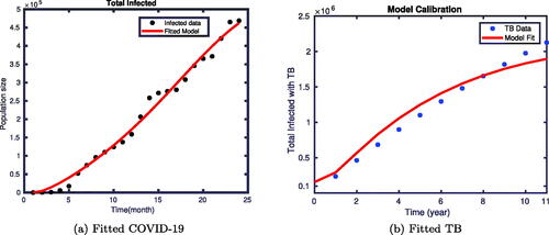
4.1. Parameter estimation

In this subsection, we estimate the parameter values of the model from the real Ethiopian data of cumulative infected cases for TB and COVID-19. The COVID-19 data is collected in a monthly time basis starting from the initial report month of March 2020 to March 2022, which is available from the source (Johns Hopkins University, 2022). Besides, the TB data is collected on a yearly basis from 2010 to 2020 and available online at the source (S. T. Partnership, 2020). To simulate the model and estimate the parameters from data, we used a least square and Bayesian combined method, as described in algorithm 1 of Mekonen, Habtemicheal, and Balcha (2021), and a nonlinear curve fitting method with the help of “fminsearch”, builtin MATLAB function. Some of the parameter values are estimated from literature as follows. According to the data by Worldometer, the Ethiopian average life expectancy at birth for 2020 is 67.07 (Deressa & Duressa, 2021; Macrotrends, 2020) and we use a sub-total population of 5,160,563. Therefore, the natural death rate of individuals per month is estimated as the reciprocal of the life expectancy individuals per time months, which is given by $\mu =\frac{1}{67.08\times 12}=0.0012.$ We approximated the recruitment rate from $\frac{\Lambda }{\mu }$ gives the initial population, to obtain $\Lambda =6,193$ individuals per month. Due to the scarcity of coinfection data, some co-infected related parameters are assumed and the others are estimated with the real data. In the estimation process, we use the initial conditions of the state variables as given in Table 2.

Table 2. The initial values for the model state variables of Equation (1)(1) $$\{\begin{array}{l}\frac{dS}{dt}=\Lambda -({\lambda }_T+{\lambda }_C+\mu )S,\\ \frac{d{L}_T}{dt}={\lambda }_{T}S-(\mu +\alpha +\eta {\lambda }_C+\omega )L_T,\\ \frac{d{I}_T}{dt}=\alpha L_T+q\sigma L_{TC}+n\tau I_{TC}-(\mu +\theta +{\delta }_T+\gamma )I_T,\\ \frac{d{E}_C}{dt}={\lambda }_{C}S-(\mu +ϵ{\lambda }_T+\phi +\pi )E_C,\\ \frac{d{I}_C}{dt}=\phi E_C+p\sigma L_{TC}+m\tau I_{TC}-(\mu +{\delta }_C+\nu +\psi )I_C,\\ \frac{d{L}_{TC}}{dt}=\eta {\lambda }_C{L}_T+ϵ{\lambda }_T{E}_C-(\mu +{\delta }_C+\rho +\sigma )L_{TC},\\ \frac{d{I}_{TC}}{dt}=\rho L_{TC}+\theta I_T+\nu I_C-(\mu +{\delta }_{TC}+\tau )I_{TC},\\ \frac{dR}{dt}=\omega L_T+\pi E_C+\gamma I_T+\psi I_C+(1-(p+q))\sigma L_{TC}+(1-(m+n))\tau I_{TC}-\mu R.\end{array}$$(1) .

State variable	S	LT	IT	EC	IC	ETC	ITC	R
Initial values	4,605,410	300,000	235,000	96	26	25	6	20,000

Figure 1 shows the fitting of the cumulative infected individuals with COVID-19, and cumulative infected population with TB of the proposed model. Figure 1(a) depicts the fitting of the infected COVID-19 model output to the observed data of COVID-19 infected population. Furthermore, the fitting of the observed data for the infected population with TB and the model simulation is shown in 1(b). In both cases, continuous lines depict the output of the model simulation, while the dotted lines act for the actual observed data of the two diseases obtained from Ethiopia. We saw that the model simulation and the actual data fit very well.

Figure 1. Model fitting using reported data of COVID-19 and TB.

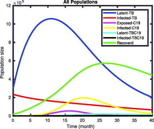
4.2. Numerical solutions of the model without control

The numerical solutions of the model Equation (1)(1) $$\{\begin{array}{l}\frac{dS}{dt}=\Lambda -({\lambda }_T+{\lambda }_C+\mu )S,\\ \frac{d{L}_T}{dt}={\lambda }_{T}S-(\mu +\alpha +\eta {\lambda }_C+\omega )L_T,\\ \frac{d{I}_T}{dt}=\alpha L_T+q\sigma L_{TC}+n\tau I_{TC}-(\mu +\theta +{\delta }_T+\gamma )I_T,\\ \frac{d{E}_C}{dt}={\lambda }_{C}S-(\mu +ϵ{\lambda }_T+\phi +\pi )E_C,\\ \frac{d{I}_C}{dt}=\phi E_C+p\sigma L_{TC}+m\tau I_{TC}-(\mu +{\delta }_C+\nu +\psi )I_C,\\ \frac{d{L}_{TC}}{dt}=\eta {\lambda }_C{L}_T+ϵ{\lambda }_T{E}_C-(\mu +{\delta }_C+\rho +\sigma )L_{TC},\\ \frac{d{I}_{TC}}{dt}=\rho L_{TC}+\theta I_T+\nu I_C-(\mu +{\delta }_{TC}+\tau )I_{TC},\\ \frac{dR}{dt}=\omega L_T+\pi E_C+\gamma I_T+\psi I_C+(1-(p+q))\sigma L_{TC}+(1-(m+n))\tau I_{TC}-\mu R.\end{array}$$(1) without implementing the optimal control are given in Figure 2. We observed from the figures that, without applying control interventions, the infected classes increase until the ${20}^{th}$ simulation time and then stabilize the number of populations in the class. The TB and COVID-19 co-infected individuals increase from the initial state and reach the pick at the ${35}^{th}$ simulation time.

Figure 2. Numerical simulations of the model.

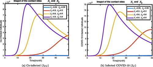
In Figure 3, we have shown that the impact of contact rates of the disease with infected compartments of the deterministic model (1). We have seen that the infected states I_C, and I_TC increase as the contact rates of the diseases increases.

Figure 3. The dynamics of I_TC and I_C with different values of the contact rates.

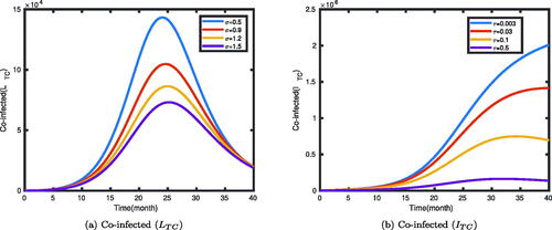
The impact of the rates (σ and τ) at which individuals leave the co-infected classes L_TC and I_TC are illustrated in Figure 4. It was shown that an increase in the leaving rate of the compartment will decrease the number of co-infected individuals. The rates σ and τ are the transfer rates of the two classes of individuals to other compartments through treatment or natural recovery. In Figure 4(a), as the transfer rate decreases from 1.5 to 0.5, the number of latent TB individuals co-infected with symptomatic COVID-19 increases, and then decreases to stabilize at some level. Similarly, if the rate τ is half, then the number of TB and COVID-19 co-infected people initially increases to a stable value at some level over time. But we can observe from Figure 4(b), as the transfer rate decreases from 0.5 to 0.003, the number of individuals who get co-infected with the two diseases increases, and stabilizes to some level.

Figure 4. The dynamics of L_TC and I_TC individuals with the values of σ and τ as given in the legend.

4.3. Numerical solutions of the control induced model

Here, we present numerical simulations for the control induced model (6) satisfying Equations (7)(7) $$P(u)=\underset{u}{\min }{\int }_0^{t_f}\left[w_1{I}_T(t)+w_2{I}_C(t)+w_3{L}_{TC}(t)+w_4{I}_{TC}(t)+\frac{1}{2}\sum _{i=1}^4{b}_i{u}_i^2\right]dt$$(7) and (8)(8) $$P(u^{*})=\min P(u)|u=(u_1,u_2,u_3,u_4)\in \Gamma$$(8) . For this, we used the initial values given in Table 2, and the parameters value as given in Table 3. The weighted coefficients of the infected individuals are assumed to be $w_1=10,w_2=35,w_3=15$ and $w_{1}4=60;$ while $b_1=100,b_2=300,b_3=500$ and $b_4=700$ for simulation purpose.

Table 3. Parameter values of the model Equation (1)(1) $$\{\begin{array}{l}\frac{dS}{dt}=\Lambda -({\lambda }_T+{\lambda }_C+\mu )S,\\ \frac{d{L}_T}{dt}={\lambda }_{T}S-(\mu +\alpha +\eta {\lambda }_C+\omega )L_T,\\ \frac{d{I}_T}{dt}=\alpha L_T+q\sigma L_{TC}+n\tau I_{TC}-(\mu +\theta +{\delta }_T+\gamma )I_T,\\ \frac{d{E}_C}{dt}={\lambda }_{C}S-(\mu +ϵ{\lambda }_T+\phi +\pi )E_C,\\ \frac{d{I}_C}{dt}=\phi E_C+p\sigma L_{TC}+m\tau I_{TC}-(\mu +{\delta }_C+\nu +\psi )I_C,\\ \frac{d{L}_{TC}}{dt}=\eta {\lambda }_C{L}_T+ϵ{\lambda }_T{E}_C-(\mu +{\delta }_C+\rho +\sigma )L_{TC},\\ \frac{d{I}_{TC}}{dt}=\rho L_{TC}+\theta I_T+\nu I_C-(\mu +{\delta }_{TC}+\tau )I_{TC},\\ \frac{dR}{dt}=\omega L_T+\pi E_C+\gamma I_T+\psi I_C+(1-(p+q))\sigma L_{TC}+(1-(m+n))\tau I_{TC}-\mu R.\end{array}$$(1) .

Parameter	Value	Source	Parameter	Value	Source
Λ	6193	Calculated	μ	0.0012	Calculated
β1	3.75	Fitted	β2	0.4372	Fitted
$\phi$	1.60	Fitted	θ	0.1229	Assumed
δC	0.009	Fitted	δt	0.0018	Fitted
ψ	0.1393	Fitted	α	0.0039	Fitted
η	1.01	Assumed	σ	1.3523	Assumed
ϵ	1.06	Assumed	ν	0.0299	Assumed
τ	0.0422	Assumed	δtc	0.002	Assumed
ρ	1.1148	Assumed	π	0.20	Fitted
ω	0.0244	Fitted	γ	0.0031	Fitted

To examine the impacts of several control strategies to mitigate the spread of the two diseases, we considered the following four scenarios.

• Scenario A (implementation of single control)

  • – Strategy 1: practicing only TB prevention methods ($u_1\ne 0,u_2=u_3=u_4=0$).

  • – Strategy 2: practicing COVID-19 only prevention methods ($u_1=0,u_2\ne 0,u_3=u_4=0$).

  • – Strategy 3: practicing medical care for TB infected individuals ($u_1=0,u_2=0,u_3\ne 0,u_4=0$).

  • – Strategy 4: applying treatment effort for COVID-19($u_1=0,u_2=0,u_3=0,u_4\ne 0$).

• Scenario B (implementation of double controls)

  • – Strategy 5: applying both the COVID-19 and TB prevention methods ($u_1\ne 0,u_2\ne 0,u_3=0,u_4=0$).

  • – Strategy 6: applying the TB prevention methods and medical care for TB infections ($u_1\ne 0,u_2=0,u_3\ne 0,u_4=0$).

  • – Strategy 7: applying the TB prevention methods and COVID-19 treatment measures ($u_1\ne 0,u_2=0,u_3=0,u_4\ne 0$).

  • – Strategy 8: applying COVID-19 prevention methods and medical care for TB infections ($u_1=0,u_2\ne 0,u_3\ne 0,u_4=0$).

  • – Strategy 9: practicing COVID-19 prevention methods and COVID-19 treatment effort ($u_1=0,u_2\ne 0,u_3=0,u_4\ne 0$).

  • – Strategy 10: implementing medical care for TB infections and applying COVID-19 treatment effort ($u_1=0,u_2=0,u_3\ne 0,u_4\ne 0$).

• Scenario C (implementation of triple controls)

  • – Strategy 11: applying both the COVID-19 and TB prevention methods, and implementing medical care for TB infected individuals ($u_1\ne 0,u_2\ne 0,u_3\ne 0,u_4=0$).

  • – Strategy 12: applying both the COVID-19 and TB prevention methods, and practicing COVID-19 treatment measures ($u_1\ne 0,u_2\ne 0,u_3=0,u_4\ne 0$).

  • – Strategy 13: applying COVID-19 prevention methods, implementing medical care for TB infected individuals, and practicing COVID-19 treatment measures ($u_1\ne 0,u_2=0,u_3\ne 0,u_4\ne 0$).

  • – Strategy 14: applying COVID-19 prevention methods, implementing medical care for TB infected individuals, and practicing COVID-19 treatment effort ($u_1=0,u_2\ne 0,u_3\ne 0,u_4\ne 0$).

• Scenario D (implementation of all controls)

  • – This scenario we consider the combination of all control means at the time. That is, $u_1\ne 0,u_2\ne 0,u_3\ne 0,u_4\ne 0.$

4.3.1. Scenario A

The simulation results of infected and co-infected individuals via the implementation of single control interventions are plotted in Figure 5. Figure 5(a) illustrates that infected individuals with TB decrease notably compared to those without applying time dependent controls measures. We also note in Figure 5(b) that COVID-19 infected individuals in the presence of optimal control measures will lead to a significant decrease over time compared to those without applying the controls.

Figure 5. Solutions of infected TB, infected COVID-19 and co-infected TB and COVID-19 individuals with single control strategy.

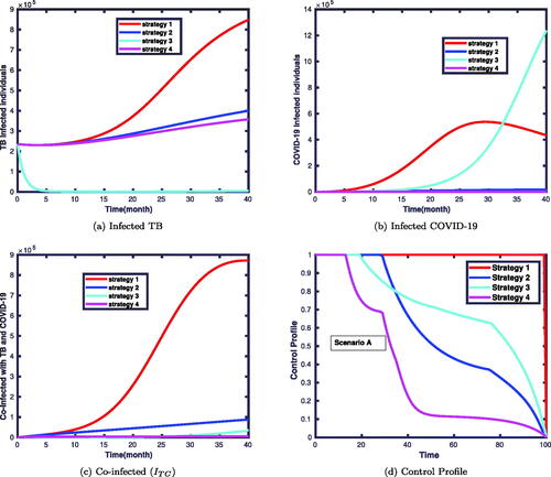
Prevention mechanisms of COVID-19 and treatments for both diseases are more effective compared to TB prevention. This is because the treatment for TB and COVID-19 makes the infected individuals recover from the infection. This effect is shown in Figure 5(c). However, the combinations of both TB and COVID-19 prevention and treatment control strategies have a remarkable influence on the prevalence of coinfection. Moreover, when only TB preventive control is used, the impact seems negligible at the beginning but one gets a significant effect after a while. This is due to prevention influences the spread of the disease after some time stages. In the beginning, the prevalence of coinfection Figure 5(c) with and without TB prevention goes at the same level, but later, one can observe its impact. The corresponding control profiles are depicted in Figure 5(d). It is clear from this figure that the profile of the control starts at its maximum values u_i = 1 and remains maximal for $(0\le t\le 20)$ in each strategy. Then, it gradually declines and drops to zero about the final time for strategies 2, 3 and 4. This suggests that to attain the expected outcomes, the control efforts need to be implemented initially at their maximum effort and then relaxed slowly until it comes to zero. The control profile for strategy 1 shows that the control term should be kept at 1 for the entire simulation period.

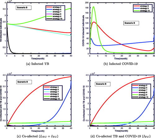
4.3.2. Scenario B

In this scenario, we considered a combination of two control functions. The simulation results are displayed in Figure 6(a)–(d). This reveals that the number of co-infected individuals was significantly reduced, as shown in these figures. Figure 6(a) shows that strategy 9 takes more time to reduce the number of infected individuals with TB compared to strategy 6. In contrast, Figure 6(b) shows that strategy 9 has a good gain compared to strategy 6 in declining the number of COVID-19 infected individuals. In Figure 6(c) and (d), strategy 5 takes more time to reduce the number of co-infected individuals compared to strategy 10. We observe that the strategy with the highest number of co-infected individuals with the diseases are strategies 5 and 6 compared to strategies 8 and 10.

Figure 6. The dynamics of infected TB, infected COVID-19 and the coinfection of TB and COVID-19 individuals, with applying two of the control strategies.

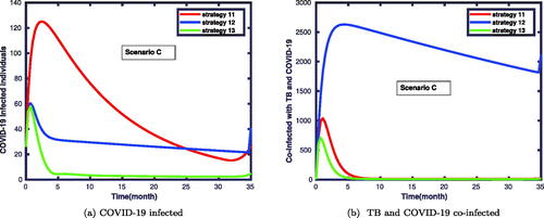
4.3.3. Scenario C

In Figure 7, we conducted numerical simulations considering the application of three control functions. In this case, one can observe that there is a slight variation among the outcomes of strategies 11, 12 and 13, as shown in Figure 7(a). Similarly, Figure 7(b) displays the variation with the effectiveness of strategies 12, 13 and 14 in combating the coinfections of TB and COVID-19. Hence, the simulation results confirm that the strategies 11 and 13 have relatively a good approach to halting the prevalence of TB and COVID-19 coinfection.

Figure 7. Simulation result when scenario C is applied on TB and COVID-19 co-dynamics.

4.3.4. Scenario D

In this scenario, we compare the simulations of the target compartments with and without controls. In this case, we apply all controls at the same time and study their impact on this coinfection. The simulation results revealed that the size of the co-infected population was significantly reduced, as shown in Figure 8. As it can be seen in Figure 8(a)–(d), the prevalence of both diseases was significantly reduced.

Figure 8. This displays the impacts of strategy 15 on: infected with TB, COVID-19, coinfection of both disease, susceptible and recovered classes.

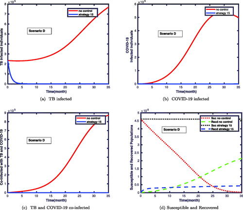
We noticed in Figure 8(a) that the number of infected individuals with TB vastly reduces when one applies simultaneously four of the controls. Figure 8(b) also shows that the COVID-19 infected individuals can be eliminated within a short time when we simultaneously implement all control measures. In particular, Figure 8(c) shows the impact of strategy 15 on the co-dynamics of TB and COVID-19. Clearly, the number of co-infected individuals drastically decreased which shows the effectiveness of the proposed strategy.

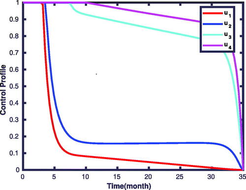
Figure 8(d) shows that numerous susceptible populations go to the infectious classes in the absence of controls. Besides, the number of recovered individuals is also increasing. However, applying the control measures decreases the susceptible population for being infected with the diseases, and hence the number of recovered populations also less compared to the first case. The corresponding control profiles for strategy 15 are given in Figure 9. Initially, the profiles take the maximum amounts to be implemented, and nearly after the $5^{th}$ time levels, the controls of u₁, and u₂ decrease gradually to the values of 0.2. After this time level, they stabilize and slowly drop to the zeroth level until the final implemented time. We have observed from the figure that the control profile for u₃, and u₄ takes the maximum value and decreases to a value of 0.9 on the ${10}^{th}$ time, and then gradually drops to its minimum value till the final time level.

Figure 9. Associated controls profile for strategy 15 of the governing system.

5. Conclusion

In this paper, we extended the deterministic coinfection model of TB and COVID-19 into an optimal control problem. The well posedness and epidemiological meaningfulness of the proposed model was proved by showing the existence, positivity and boundedness of all solutions in the feasible region. The impacts of both diseases were analyzed comparatively. The analytical results reveal that there is a positive impact on one disease to the other in spreading the diseases. To reduce the prevalence of the diseases, we extended into an optimal control model by including four control functions, in the form of prevention and treatment. Prevention controls are applied to the susceptible and exposed classes, while the treatment mechanisms are applied to the infected and co-infected ones. The optimal control functions are, then computed by minimizing the number of active TB infected, latent TB and COVID-19 co-infected, COVID-19 infected and active TB and COVID-19 co-infected populations by considering the cost of interventions. Then, the existence of optimal controls and their characterization are discussed analytically. The constrained problem is characterized via the application of Pontryagin’s Minimum Principle, and we have obtained an optimality system that satisfies the necessary conditions.

Furthermore, we numerically simulated our mathematical model using estimated and assumed parameter values, and suitable initial conditions for the case of Ethiopia. From our simulation results, we conclude that decreasing the effective contact rates, and increasing the recovery rates of the two diseases, has a big contribution to minimize their spread. The numerical solution of the optimal control problem was solved with a forward-backward sweep method. Numerical simulations of the optimal control extended model indicate that the prevention and treatment interventions are effective in reducing the transmission for the coinfection of the diseases, so we may get maximum disease control that the control measures are applied. Therefore, it could be concluded that the effective implementation of prevention efforts against TB, COVID-19 prevention mechanisms, treatment efforts for infected individuals with TB, and medical care for COVID-19 infections as control strategies could help to minimize the coinfection of both diseases and disease induced difficulties.

This study can be extended into a delayed model, by introducing time delays in the awareness level of individuals towards self-protection behaviour changes. It can also be extended to a fractional-order model to study the memory effects of the biological systems, and stochastic differential equations for the developed model are recommended for further study.

Declaration of competing interest

The authors would declare that they have no competing interests that could appeared to influence this work.

Acknowledgments

The first author acknowledges Adama Science and Technology University under grant number ASTU/SP-R/120/21, and the Simon’s foundation fellowship through Research and Graduate studies in mathematics and its applications (RGSMA), Botswanan International University of Science and Technology (BIUST), for their financial support.

Availability of data and materials

The data used to support the findings of this study are included within the sections of the article and available in Johns Hopkins University (2022) and S. T. Partnership (2020).

References

- Abdullahi Baba, I., Nasidi, B. A., & Baleanu, D. (2021). Optimal control model for the transmission of novel COVID-19. Computers, Materials, & Continua, 66, 3089–3106. doi:10.32604/cmc.2021.012301
- Ain, Q. T., Anjum, N., Din, A., Zeb, A., Djilali, S., & Khan, Z. A. (2022). On the analysis of Caputo fractional order dynamics of middle east lungs coronavirus (MERS-CoV) model. Alexandria Engineering Journal, 61(7), 5123–5131. doi:10.1016/j.aej.2021.10.016
- Akgül, A., Ahmed, N., Raza, A., Iqbal, Z., Rafiq, M., Baleanu, D., & Rehman, M. A.-u. (2021). New applications related to COVID-19. Results in Physics, 20, 103663. doi:10.1016/j.rinp.2020.103663
- Asamoah, J. K. K., Okyere, E., Abidemi, A., Moore, S. E., Sun, G.-Q., Jin, Z., … Gordon, J. F. (2022). Optimal control and comprehensive cost-effectiveness analysis for COVID-19. Results in Physics, 33, 105177. doi:10.1016/j.rinp.2022.105177
- Beyne, N. W., Sitota, A. L., Tegegn, B., & Bobobsha, K. (2021). The impact of COVID-19 on the tuberculosis control activities in Addis Ababa. Pan African Medical Journal, 38. doi:10.11604/pamj.2021.38.243.27132
- Chen, Y., Wang, Y., Fleming, J., Yu, Y., Gu, Y., Liu, C., … Liu, Y. (2020). Active or latent tuberculosis increases susceptibility to COVID-19 and disease severity. doi:10.1101/2020.03.10.20033795
- Cilloni, L., Fu, H., Vesga, J. F., Dowdy, D., Pretorius, C., Ahmedov, S., … Arinaminpathy, N. (2020). The potential impact of the COVID-19 pandemic on the tuberculosis epidemic a modelling analysis. eClinicalMedicine, 28, 100603. doi:10.1016/j.eclinm.2020.100603
- Deressa, C. T., & Duressa, G. F. (2021). Modeling and optimal control analysis of transmission dynamics of COVID-19: The case of Ethiopia. Alexandria Engineering Journal, 60(1), 719–732. doi:10.1016/j.aej.2020.10.004
- Fatima, B., & Zaman, G. (2020). Co-infection of middle eastern respiratory syndrome coronavirus and pulmonary tuberculosis. Chaos, Solitons, and Fractals, 140, 110205. doi:10.1016/j.chaos.2020.110205
- Feldman, C., & Anderson, R. (2021). The role of co-infections and secondary infections in patients with COVID-19. Pneumonia, 13(1). doi:10.1186/s41479-021-00083-w
- Fleming, W. H., & Rishel, R. W. (2012). Deterministic and stochastic optimal control (Vol. 1). New York, Heidelberg, Berlin: Springer Science & Business Media.
- Fund, T. G. (2021, September 08). Global fund results report reveals COVID-19 devastating impact on HIV, TB and malaria programs, results report 2021 [Tech. Rep.]. Geneva: The Global Fund.
- Gaff, H., & Schaefer, E. (2009). Optimal control applied to vaccination and treatment strategies for various epidemiological models. Mathematical Biosciences and Engineering, 6(3), 469–492. doi:10.3934/mbe.2009.6.469
- Goudiaby, M., Gning, L., Diagne, M., Dia, B. M., Rwezaura, H., & Tchuenche, J. (2022). Optimal control analysis of a COVID-19 and tuberculosis co-dynamics model. Informatics in Medicine Unlocked, 28, 100849. doi:10.1016/j.imu.2022.100849
- Johns Hopkins University. (2022). Johns Hopkins University Coronavirus Resource Center. Coronavirus cases-Ethiopia. Retrieved from https://www.indexmundi.com/coronavirus/country/et
- Khurana, A. K., & Aggarwal, D. (2020). The (in)significance of TB and COVID-19 co-infection. European Respiratory Journal, 56(2), 2002105. doi:10.1183/13993003.02105-2020
- Kifle, Z. S., & Obsu, L. L. (2022). Mathematical modeling for COVID-19 transmission dynamics: A case study in Ethiopia. Results in Physics, 34, 105191. doi:10.1016/j.rinp.2022.105191
- Lenhart, S., & Workman, J. T. (2007). Optimal control applied to biological models. London: CRC Press, Taylor & Francis Group.
- Macrotrends. Life-expectancy of Ethiopia. Retrieved from https://www.macrotrends.net/countries/ETH/ethiopia/life-expectancy
- Marimuthu, Y., Nagappa, B., Sharma, N., Basu, S., & Chopra, K. K. (2020). COVID-19 and tuberculosis: A mathematical model based forecasting in Delhi, India. The Indian Journal of Tuberculosis, 67(2), 177–181. doi:10.1016/j.ijtb.2020.05.006
- Mekonen, K. G., Balcha, S. F., Obsu, L. L., & Hassen, A. (2022). Mathematical modeling and analysis of TB and COVID-19 coinfection. Journal of Applied Mathematics, 2022, 1–20. doi:10.1155/2022/2449710
- Mekonen, K. G., Habtemicheal, T. G., & Balcha, S. F. (2021). Modeling the effect of contaminated objects for the transmission dynamics of COVID-19 pandemic with self protection behavior changes. Results in Applied Mathematics, 9, 100134. doi:10.1016/j.rinam.2020.100134
- Nana-Kyere, S., Boateng, F. A., Jonathan, P., Donkor, A., Hoggar, G. K., Titus, B. D., … Adu, I. K. (2022). Global analysis and optimal control model of COVID-19. Computational and Mathematical Methods in Medicine, 2022, 1–20. doi:10.1155/2022/9491847
- Obsu, L. L., & Balcha, S. F. (2020). Optimal control strategies for the transmission risk of COVID-19. Journal of Biological Dynamics, 14(1), 590–607. doi:10.1080/17513758.2020.1788182
- Okosun, K., & Makinde, O. (2014). A co-infection model of malaria and cholera diseases with optimal control. Mathematical Biosciences, 258, 19–32. doi:10.1016/j.mbs.2014.09.008
- Omame, A., Abbas, M., & Onyenegecha, C. (2021). A fractional-order model for COVID-19 and tuberculosis co-infection using Atangana-Baleanu derivative. Chaos, Solitons, and Fractals, 153, 111486. doi:10.1016/j.chaos.2021.111486
- Pontryagin, L. S. (2018). Mathematical theory of optimal processes. Boca Raton, RL: Routledge.
- S. T. Partnership. (2020). Tuberculosis situation in Ethiopia, 2010-2020. Retrieved from https://www.stoptb.org/static_pages/ETH_Dashboard.html
- Schroers, B. J. (2011). Ordinary differential equations: A practical guide. Cambridge: Cambridge University Press.
- Sharomi, O., & Malik, T. (2017). Optimal control in epidemiology. Annals of Operations Research, 251(1-2), 55–71. doi:10.1007/s10479-015-1834-4
- Silva, C. J., & Torres, D. F. M. (2014). Modeling TB-HIV syndemic and treatment. Journal of Applied Mathematics, 2014, 1–14. doi:10.1155/2014/248407
- Tadolini, M., García-García, J.-M., Blanc, F.-X., Borisov, S., Goletti, D., Motta, I., … Migliori, G. B. (2020). On tuberculosis and COVID-19 co-infection. European Respiratory Journal, 56(2), 2002328. doi:10.1183/13993003.02328-2020
- Treesatayapun, C. (2022). Epidemic model dynamics and fuzzy neural-network optimal control with impulsive traveling and migrating: Case study of COVID-19 vaccination. Biomedical Signal Processing and Control, 71, 103227. doi:10.1016/j.bspc.2021.103227
- Visca, D., Ong, C. W. M., Tiberi, S., Centis, R., D'Ambrosio, L., Chen, B., … Goletti, D. (2021). Tuberculosis and COVID-19 interaction: A review of biological, clinical and public health effects. Pulmonology, 27(2), 151–165. doi:10.1016/j.pulmoe.2020.12.012
- World Health Organization (2021, May 5). WHO information note: COVID-19: Considerations for tuberculosis (TB) care [Tech. Rep]. WHO-2019-nCoV-TB-care-2021.1, WHO.
- World Health Organization. (2020). World Health Organization (WHO) information note tuberculosis and COVID-19.
- World Health Organization. (2020, June 5). Advice on the use of masks in the context of COVID-19: Interim guidance [Tech. Rep.]. WHO/2019-nCoV/IPC_Masks/2020.4. World Health Organization.
- World Health Organization. (March 2020). Key messages and actions for COVID-19 prevention and control in schools. UNICEF/UNI220408/Pacific, UNICEF, WHO, IFRC.