
 ?Mathematical formulae have been encoded as MathML and are displayed in this HTML version using MathJax in order to improve their display. Uncheck the box to turn MathJax off. This feature requires Javascript. Click on a formula to zoom.
Abstract
Traditionally, partial differential equation (PDE) problems are solved numerically through a discretization process. Iterative methods are then used to determine the algebraic system generated by this process. Recently, scientists have emerged artificial neural networks (ANNs), which solve PDE problems without a discretization process. Therefore, in view of the interest in developing ANN in solving PDEs, scientists investigated the variations of ANN which perform better than the classical discretization approaches. In this study, we discussed three methods for solving PDEs effectively, namely Pydens, NeuroDiffEq and Nangs methods. Pydens is the modified Deep Galerkin method (DGM) on the part of the approximate functions of PDEs. Then, NeuroDiffEq is the ANN model based on the trial analytical solution (TAS). Lastly, Nangs is the ANN-based method which uses the grid points for the training data. We compared the numerical results by solving the PDEs in terms of the accuracy and efficiency of the three methods. The results showed that NeuroDiffeq and Nangs have better performance in solving high-dimensional PDEs than the Pydens, while Pydens is only suitable for low-dimensional problems.
1. Introduction
Many physical phenomena in modern sciences have been described by using Partial Differential Equations (PDEs) (Evans, Blackledge, & Yardley, Citation2012). Hence, the accuracy of PDE solutions is challenging among the scientists and becomes an interest field of research (LeVeque & Leveque, Citation1992). Traditionally, the PDEs are solved numerically through discretization process (Burden, Faires, & Burden, Citation2015),. For instance, the well-known finite difference method (FDM) and finite element method were utilized to solve many PDE linear and non-linear. Other methods, such as the variational iteration method (VIM) and its variations were used to solve the nonlinear PDE (He & Latifizadeh, Citation2020), and the finite difference-spectral method was investigated to solve the fractal mobile and immobile transport (Fardi & Khan, Citation2021). These methods typically end up with the algebraic systems that can be solved by using iterative methods (Hayati & Karami, Citation2007). The big issue in using the iterative solvers for solving the large scale of linear system of equations is that they potentially breakdown before getting a good approximate solution (Maharani & Salhi, Citation2015). In fact, their accuracy is not promising. To get rid of the breakdown problem, one has been done by using interpolation and extrapolation model (Bakar & Salhi, Citation2019; Maharani et al., Citation2018; Maharani, Larasati, Salhi, & Khan, Citation2019), and using prediction with support vector machine (Thalib, Bakar, & Ibrahim, Citation2021). However, the problem is still not fully addressed since computationally, they quite expensive. With no discretization process, artificial neural networks (ANNs) can be an alternative way.
ANN is well-known as one method under machine learning (ML) which is typically used for regressions and classification problems. The development of ANN for solving PDE problems has been investigated at the beginning of the 21st century. For instance (Malek & Beidokhti, Citation2006), combined ANN and Nelder–Mead simplex method to find the numerical solutions of the high-order of PDE. This hybrid method improved the ANN performances by approximating initial and boundary conditions. Moreover (Sirignano & Spiliopoulos, Citation2018), used the Deep-Galerkin method (DGM) embedded with ANN, for solving the high dimensional of PDE problems. While, modified DGM by introducing ansatz method for binding the initial and boundary conditions. This modification simplifies the DGM original algorithm. Furthermore, another ANN-based method for solving PDE, called Physics Informed Neural Network (PINN), was introduced by Raissi, Perdikaris, & Karniadakis (2017b), Raissi, Perdikaris, and Karniadakis (Citation2019) and Raissi et al. (2017b). PINN considers the physical laws of PDE to be embedded in loss function as a regularization term. This method was improved by Guo, Cao, Liu, and Gao (Citation2020), in terms of the training effect by using the residual-based adaptive refinement (RAR) method. This strategy will impact in increasing the number of residual points with the large residuals of PDE until the residuals are less than the threshold.
The ability of ANN in solving PDE problems gives some advantages, including continuous and differentiable of the approximate solutions, good interpolation characteristics and less memory (Chen et al., Citation2020). Other advantages of ANN are that it can utilize automatic differentiation tools, such as Tensorflow (Abadi et al., Citation2016) and PyTorch (Paszke et al., Citation2017; Rahaman et al., Citation2019), allow researchers make more simpler methods in solving PDE problems (Chen et al., Citation2020). In this study, we focus on three methods for solving PDEs based on ANN model, namely PyDEns which modifies the DGM, NeuroDiffEq which is the ANN approximator with TAS applied (Chen et al., Citation2020), and Nangs which based on the grid points for training data).
This article is structured by follows. Section 1 discusses introduction of ANN-based methods for solving PDEs. Section 2 describes the review of ANN to solve PDEs. In Section 3, the basic theory behind the three methods is also discussed. Section 4 illustrates the three methods solve the heat equation. The numerical results of the three methods in solving different types of PDEs are explained in Section 5. Lastly, we conclude our study in Section 6.
2. Artificial neural networks (ANN)
ANNs were introduced firstly in 1943 by McCulloch and Pitts (Citation1943). It is inspired by biological neurons working to perform complex tasks (Schalkoff, Citation1997). At the beginning, ANN has been successful handling several data problems, which then becomes less popular since left out behind another ML techniques. In 1980s, with the tremendous increase in computing power and the amount of data used to training ANNs, this technique became more popular and was successfully applied in various practical applications (Goodfellow, Bengio, & Courville, Citation2016; Goldberg, Citation2016; Helbing & Ritter, Citation2018; LeCun, Bengio, & Hinton, Citation2015; Li et al., Citation2019; Mabbutt, Picton, Shaw, & Black, Citation2012; Nielsen, Citation2015; Shanmuganathan, Citation2016), including the differential equation problems discussed in this article.
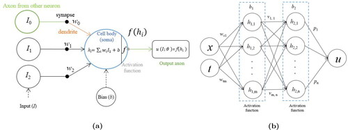
One of the most popular ANN architecture called Perceptron, as shown in (Haykin, Citation1999), consists of multiple hidden layers as visualized in (Khanna, Citation1990),. However, prior to the invention of the backpropagation algorithm (Rumelhart, Hinton, & Williams, Citation1985), it was not easy for training perceptron to make a better prediction. In short, backpropagation is a gradient descent method, which enables the perceptron to give a better approximation based on the gradient of the loss function. Furthermore, the backpropagation algorithm became the most popular ANN optimizer algorithm (Li, Cheng, Shi, & Huang, Citation2012; Nielsen, Citation2015).
Figure 1. ANN Perceptron 1 (a) and multi-layered perceptron (MLP) 1 (b) architectures.
2.1. Ann model for solving PDEs: overview
Consider the second-order PDE of the form (McFall, Citation2010),
(1)
(1)
over the domain
with an initial condition
(2)
(2)
and a boundary condition
(3)
(3)
Generally, ANN to solve PDE (Equation (1)) is started by generating the weights to form a linear combination with the inputs x, t and the bias, bi. This form is then used to compute the hidden layer as described in EquationEquation (4)(4)
(4) as follows
(4)
(4)
where h1 is the first hidden layer, wxi and wti are the weights and b1 is bias. The second hidden layer, as expressed in Equation (5), is computed by feeding h1 into it and thus is processed to yield the output layer.
(5)
(5)
where vij are the weights, b2 is the bias, and f is the activation function of the form
(6)
(6)
The activation functions are commonly used to perform the diverse of computations between the layers. Several activation function, such as sigmoid or logistic, tanh, ReLU and Leaky-ReLU are often used (Haykin, Citation1999; Jagtap, Kawaguchi, & Karniadakis, Citation2020). Here, we take the hyperbolic tangent function (tanh) as it has been proved to provide the better results compared to other activation functions (Karlik & Olgac, Citation2011; Panghal & Kumar, Citation2021).
Our aim here is to obtain the approximate solution which is written as follows,
(7)
(7)
where pj are the weights of the output layers. To control the accuracy of the approximate solution, we compare it with the right-hand side of the PDE (Equation (1)), and this can be only done by differentiate partially
as follows
(8)
(8)
(9)
(9)
where k = 1, 2.
3. Ann-based methods for solving PDEs
In this section, we discuss three methods and compare them in terms of accuracy and efficiency. They are Pyden, NeuroDiffeq and Nangs. They are differed by the way generating the training points and the loss functions.
3.1. Pydens method
All of ANN-based methods to solve the PDE problem used an optimizer in order to obtain the minimum error. The most common optimization method used is called Deep Galerkin Method (DGM), has been introduced by Sirignano and Spiliopoulos (Citation2018). The name of Pydens was obtained from the python module with the DGM optimizer. Basically, to approximate u(t, x) in Equation (1) using Pydens is modified by applying ansatz in binding the initial and boundary conditions. The procedure is explained as follows.
Bind the initial and boundary conditions using ansatz by setting up the equation
(10)
Thus, the solution of PDE is approximated by transforming the ANN output rather than
Generate m points inside the batches of b1 from the domain
Build the loss function as follows
Update the trainable parameter θ to minimize the loss function by using SGD optimizer.
3.2. Neurodiffeq method
NeuroDiffeq method applies the trial approximate solution (TAS) (Chen et al., Citation2020), that satisfies the initial and boundary conditions. Recall EquationEquation (1)(1)
(1) . The procedure of NeuroDiffeq method is explained as follows:
Generate m × n input points of
Build the TAS, uT, as the form of McFall (Citation2010).
Build the loss function (McFall, Citation2006).
3.3. Nangs method
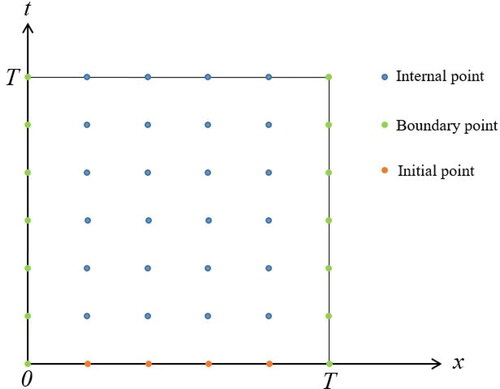
Different from both methods explained above, Nangs method is not required to create trial solution to minimize the loss functions, instead, it generates mesh points for the training data. The details of how Nangs method can approximate PDE are described as follows.
Set mesh points of
For each internal point, once feeding process has been done in ANN architecture, compare the output with the right side of the PDE using the following loss function:
For all of the initial and boundary points, the outputs are compared with EquationEquations (2)
Figure 2. Illustration of the internal, boundary and initial points of
4. Simulation of the three ANN-based methods for solving heat equation
As an illustration of using ANN-based methods to solve PDEs, the following heat equation is considered (Burden et al., Citation2015),
(22)
(22)
with the initial condition
(23)
(23)
and boundary conditions
(24)
(24)
The analytical solution for this PDE is given by
(25)
(25)
To compare the three methods, we used the same architectures of ANN which are three hidden layers consisting 32 neurons each. The loss function is evaluated up to 100 × 100 points for the unit inputs (x, t). We also used various number of iterations because each method uses different python modules. Pydens is run under Tensorflow (Abadi et al., Citation2016), while NeuroDiffeq and Nangs are run under Pytorch (Paszke et al., Citation2017).
4.1. Pydens in solving PDE heat equation
To solve PDE heat in EquationEquation (22)(22)
(22) , firstly, we use ansatz function to bind the boundary and initial conditions. We then randomly generate up to 100 × 100 number of points inside the domain
Finally, we compute the loss function as in Equation (11). The complete algorithm for this method is described in Algorithm 1.
Algorithm 1.
Pydens algorithm for solving PDE heat equation [14]
Approximate PDE (Equation (22)) by fitting u(x, t) with the following function
Generate up to
while
for
Compute the output
Substitute
Compute the loss function by comparing the Anet with EquationEquation (22)
end for
Apply the SGD to optimize the trainable parameter θ.
end while
4.2. Neurodiffeq in solving heat equation
Different from the PyDens method, NeuroDiffeq uses TAS (McFall, Citation2006), to approximate the initial and boundary conditions. Basically, once we set up the domain into 100 × 100 data points, we then construct TAS to satisfy the initial and boundary conditions 23 and 24. The details of solving the PDE heat in EquationEquation (22)
(22)
(22) are described in Algorithm 2.
Algorithm 2.
NeuroDiffeq algorithm for solving PDE heat equation [19]
Generate
Construct a TAS which satisfies the initial and boundary conditions based on Equations (23) and (24) as follows
Noted here that we used θ to indicate that it consists of the weights and the biases.
while
for each (xi, ti) do
Calculate the output of ANN
Substitute unet into uT and differentiate it to obtain
Compute the loss function by comparing the output between EquationEquations (22)–(24) as follows
end for
Apply SGD optimizer to minimize the loss function.
end while
4.3. Nangs method in solving PDE heat equation
Nangs method adopts the grid points used in the discretization process as the training data. It is done by building mesh points from (x, t) in the entire domain. Then, split the mesh points into internal, initial, and boundary points (see ). The complete algorithm is shown in Algorithm 3.
Algorithm 3.
Nangs algorithm for solving PDE heat equation [23]
Set up
while
for each mesh point
Calculate the output as follows
Differentiate the output to obtain the following functions
Calculate each internal point, then compare it with the original PDE of Equations (22) as follows
Compute each initial and boundary points and compare them with the original initial and boundary condition of the PDE as in Equations (23) and (24) as follows
end for
Apply the SGD to optimize the weight and the biases.
end while
5. Results and discussion
In this section, the three methods, PyDens, NeuroDiffeq and Nangs, are compared in terms of the accuracy and efficiency by solving several three types of PDE, namely elliptic, parabolic and hyperbolic (Burden et al., Citation2015). We also compared all three methods performance with the classical method which is FDM. All of the results are shown in various tables and figures.
5.1. Simulation results in solving PDE heat equation
The comparison methods for solving PDE heat equation as in Equations (22)–(24) are recorded in .
Table 1. The performance of PyDens, NeuroDiffeq and Nangs methods for solving PDE heat equation.
According to , Pydens was able to solve the problems most accurate between the other ANN-based methods. For instance, the loss values of Pydens when using 25 × 25, 50 × 50 and 75 × 75 training data are, respectively, and
or about 84, 87 and 72% more accurate compared with NeuroDiffeq and Nangs. In contrast, for 100 × 100 training data, the NeuroDiffeq gives the most accurate value of loss than the other methods, with the loss value
compared with
and
or about 13 and 20%, respectively. While in comparison with the classical method, FDM give better loss value only in 75 × 75 and 100 × 100 training data, which is, respectively, given by
and
().
In terms of the computational times, Pydens also gives the shortest time compared with the other two ANN-based methods, it spent 53 seconds only when using 25 × 25 training data, whereas 65 and 578 s needed for NeuroDiffeq and Nangs, respectively, for using the same training data. The higher training data of the PDE problem, such as 50 × 50, 75 × 75 and 100 × 100, need more times for the three methods. However, Pydens is still the winner between them. While in comparison with classical method, FDM is still gives the shortest time compared to ANN-based method with less than 10 s in all problems. The results are more clearly seen when we visualized the analytical solution as in and the comparisons via .
Figure 3. Analytical solution of heat equation.
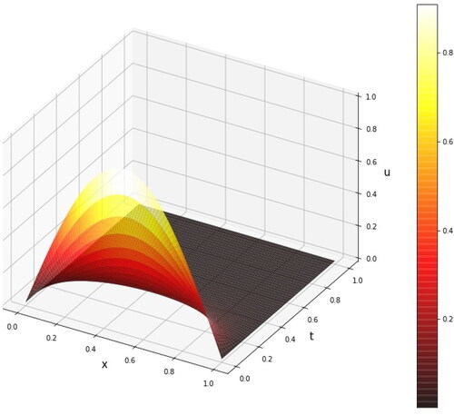
Figure 4. Comparison analytical and approximate solutions of PDE heat equation by using Pydens method.
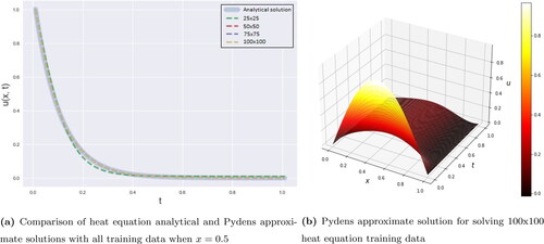
Figure 5. Comparison analytical and approximate solutions of PDE heat equation by using NeuroDiffeq method.
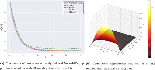
Figure 6. Comparison analytical and approximate solutions of PDE heat equation by using Nangs method.
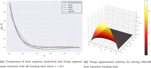
According to , all three methods almost give similar result from the analytical solution. However, from the other perspective as can be seen in when all training data are shown, all methods show a little bit different from the analytical solution. Especially in lower training data, different results give in the 100 × 100 training data when all methods are closer to the analytical solution.
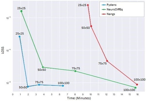
The comparison of all ANN-based methods in terms of the loss values and the computational times are shown in . As we can see here that the higher numbers of training data used for solving the PDE heat would affect the performance of the methods. It is appeared in NeuroDiffEq and Nangs methods. For Pydens method, however, it just occurred when using the lower numbers of training data, namely 25 × 25 and 50 × 50, whereas greater than that, the Pydens performance slightly worse.
Figure 7. Comparisons of the loss values and the computational times between the ANN-based methods for solving heat equation at all training points.
For further analysis of the performance of three methods, it is also shown in , where it illustrates all of the results of loss values of the variation number of hidden layers, and neurons per layer.
Table 2. The loss values of PDE Heat simulation for different number of layers and neurons.
It can be seen from , in general, when the number of layers and neurons increased, the prediction accuracy also improved. However, more complex ANN architecture causes the computational time increased. Hence, determine the best ANN architecture is crucial.
5.1.1. Simulation results in solving PDE wave equation
Wave equation is one of the hyperbolic PDE and contains the second-order partial derivatives (Guo et al., Citation2020). Wave equation has been applied in many sciences fields, such as seismic wave propagation and acoustic wave propagations (Gu, Zhang, & Dong, Citation2018; Kim, Citation2019; Li, Feng, & Schuster, Citation2017). The wave equation is described as the following equations [3]:
(26)
(26)
with initial conditions
(27)
(27)
(28)
(28)
and boundary conditions
(29)
(29)
The analytical solution is given as follows
(30)
(30)
The simulation results of the three methods to solve the wave equation are shown in .
Table 3. The performance of the three methods for solving PDE wave equation.
Similar to the previous results, in comparison with other ANN-based method, Pydens provides better performance in solving PDE wave for using 25 × 25 training data with a loss value of compared with
and
for, respectively, NeuroDiffeq and NAngs methods. It is more accurate about 94 and 98% than NeuroDiffEq and Nangs, respectively. Furthermore, for the remaining of using training data, NeuroDiffEq consistently performed well, as can be seen in , the loss values for NeuroDiffEq are
and
for 75 × 75 and 100 × 100 training data, respectively, or almost twice better than Pydens and Nangs. While compare to the classical method, FDM only performed better at 25 × 25 which is
against
that belongs to NeuroDiffEq. below support all performances of Pydens, NeuroDiffEq and Nangs methods for solving the PDE wave. It can be seen that Pydens curve get closer to the analytical curve for the lower dimension, whereas NeuroDiffEq curve gets closer to the analytical curve () in the higher dimensions.
Figure 8. Analytical solution of wave equation.
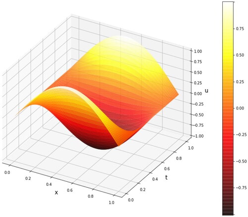
Figure 9. Comparison analytical and approximate solutions of PDE wave equation by using Pydens method.
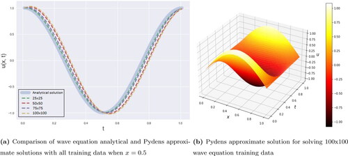
Figure 10. Comparison analytical and approximate solutions of PDE wave equation by using NeuroDiffeq method.
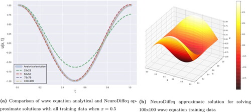
Figure 11. Comparison analytical and approximate solutions of PDE wave equation by using Nangs method.
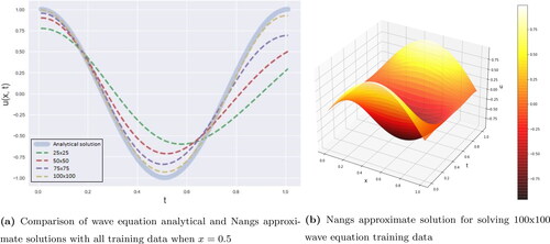
In , we can see that NeuroDiffEq closer to analytical solution from 50 × 50 to 100 × 100 training data compare to the other. Pydens in 25 × 25 training data is the best; however, the other training data gives no significant progress. Meanwhile for Nangs, all of the training data result is not close to the analytical solution.
above shows similar trends with the one in the previous section, where Pydens took the shortest time with about 61 s for 25 × 25 training data, compared with 81 and 1062 s for NeuroDiffeq and Nangs, respectively. However, NeuroDiffEq gives better results for using greater numbers of training data than the other two methods. The simulation results with different ANN architectures are shown in .
Figure 12. Comparisons of the loss values and the computational times between the ANN-based methods for solving wave equation at all training points.
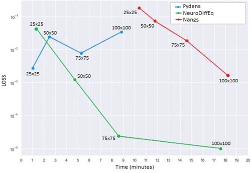
Table 4. Wave simulation results with different number of layers and neurons.
5.1.2. Simulation results in solving Poisson equation
Poisson is applied in many modern technologies (Aggarwal & Ugail, Citation2019) and in a wide area of problems from simulating fluid flows (Xiao, Zhou, Wang, & Yang, Citation2020), modelling gravitational and electrostatic fields (Blakely, Citation1996), surface reconstruction (Kazhdan, Bolitho, & Hoppe, Citation2006), image processing (Pérez, Gangnet, & Blake, Citation2003), as well as other applications in geometric design (Arnal, Monterde, & Ugail, Citation2011; Ahmat, Castro, & Ugail, Citation2014; Chaudhry et al., Citation2015; Elmahmudi & Ugail, Citation2019; Jha, Ugail, Haron, & Iglesias, Citation2018; Shen, Sheng, Chen, Zhang, & Ugail, Citation2018; Ugail & Ismail, Citation2016). The PDE Poisson, as its anaytical solution is displayed in , has the form of Elsherbeny, El-hassani, El-badry, and Abdallah (Citation2018):
(31)
(31)
with boundary conditions
(32)
(32)
Figure 13. Analytical solution of Poisson equation.
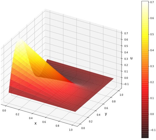
The analytical solution for this PDE is given as follows
(33)
(33)
shows detailed information of the three methods in solving Poisson equation above.
Table 5. The performance of the three methods for solving Poisson equation.
According to , all methods showed a good performance, NeuroDiffEq, however is still the most accurate with and
for using 25 × 25 numbers of training data and above. This number is 99.8, 99, 100 and 100% more accurate than the other methods. This trend is clearly seen in .
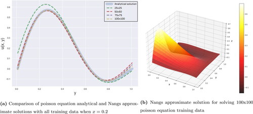
In , when we see the overall result, Pydens failed to approximate the boundary condition well. That is the reason why even Pydens show a good results at x = 0.2, the overall error is not good enough. NeuroDiffEq in is the best in this case when all of the training data result is almost similar to the analytical solution. Meanwhile for Nangs in , only 25 × 25 training data that not show a good result.
Figure 14. Comparison analytical and approximate solutions of PDE Poisson by using Pydens method.
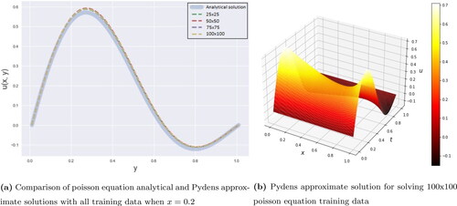
Figure 15. Comparison analytical and approximate solutions of PDE Poisson by using NeuroDiffeq method.
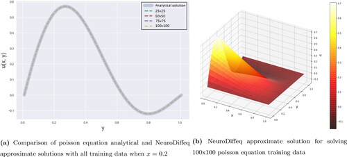
Figure 16. Comparison analytical and approximate solutions of PDE Poisson by using Nangs method.
The performances of the three methods are summarized in , when it can be seen that the NeuroDiffEq is the most accurate method to solve the Poisson EquationEquation (31)(31)
(31) . However, this method is the slowest one compared with Pydens and Nangs methods, with 1177 s for using 100 × 100 training data. Pydens, in contrast, took the shortest time which only 53 s for 25 × 25 training data, compared with 105 and 544 s for NeuroDIffeq and Nangs methods, respectively. Similarly, when using 100 × 100 training data, Pydens needs 423 s only, compared with 1177 and 967 s for the other two methods, respectively. The simulation results for using different ANN architectures are recorded in .
Figure 17. Comparisons of the loss values and the computational times between the ANN-based methods for solving Poisson equation at all training points.
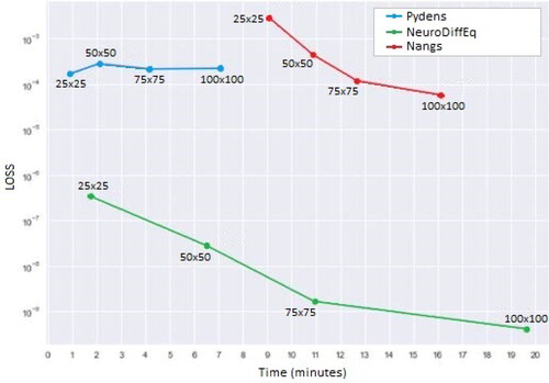
Table 6. Poisson simulation results with different number of layers and neurons.
5.2. Discussion
Overall, can be said the approximation solutions of PDE heat, PDE wave and PDE Poison equation using NeuroDiffEq give the better and stable accuracy than Pydens, Nangs, and even classical method FDM. This observation can be seen in , respectively. However, in the evaluation of the computational time, the FDM still give the shortest time compared to all ANN-based method. While comparing between the three ANN-based methods; this method took the longest when we added more training data. Furthermore, Pydens is the fastest method in solving all given problems. Unfortunately, the performance of this method is disappointing since more training data points do not affect its accuracy. Meanwhile, Nangs gives an unpredictable expectation results with its position is in the middle between the two methods. This method, in our point of view, can potentially give the better performance when solving the variety of PDE problems. The readers can see all the performances of the three methods through which clearly indicate the conditions explained above.
To further investigation of the performances of these three methods, we also ran the simulations that can be seen in , respectively. The results showed that to improve the performance of the three methods, we can also change the ANN architectures by adding more numbers of layers and neurons. However, these options will increase the computational time. Another options are to increase iteration and change the optimizer.
6. Conclusion
We have discussed Pydens, NeuroDiffEq and Nangs methods to solve the heat, wave and Poisson equations of the second order of PDEs, and also compared with classical method. The training data used ranging from 25 × 25 to 100 × 100 points. We compared the accuracy as well as the time efficiency of each method. There are advantages and disadvantages of each method based on our experiments result. In term of the accuracy, NeuroDiffEq consistently produced the lowest loss values compared with Pydens, Nangs and FDM. To get better loss values, the training data points need to be increased though. However, it affected the longer computational time. On the other hand, the classical method FDM is still given the fastest method compared with the others. Interestingly, for Nangs method, although this method is not the fastest nor the lowest loss value, but it potentially produces the better loss values for solving high dimensional problems. It can be seen on that the training data, the computation times, and the trend of loss values are potentially overtaken by NeuroDiffEq’s performance on high training data problems.
For future work, we recommend solving the smaller dimensional problems using the Pydens method because this method shows good performance. For higher dimensional problems, we recommend the NeuroDiffEq or Nangs methods. However, for NeuroDiffEq, we can see that this method is risky when using high amount of training data, affecting computation time. While for Nangs, although it does not perform very well, it is still capable of providing better performance and shorter computation time than NeuroDiffEq. Adjusting the ANN architecture, such as increasing the number of layers and neurons, can also improve the performance of ANN-based methods. However, the more complex the ANN architecture, the more expensive the method.
Disclosure statement
No potential conflict of interest was reported by the author(s).
Data availability statement
Not applicable.
References
- Abadi, M., Barham, P., Chen, J., Chen, Z., Davis, A., Dean, J., … Isard, M. (2016). Tensorflow: A system for large-scale machine learning. 12th {USENIX} symposium on operating systems design and implementation ({OSDI} 16) (pp. 265–283). Savanah, GA, US: USENIX.
- Aggarwal, R., & Ugail, H. (2019). On the solution of poisson’s equation using deep learning. 2019 13th International Conference on Software, Knowledge, Information Management and Applications (SKIMA) (pp. 1–8). Piscataway, NJ: IEEE. doi:10.1109/SKIMA47702.2019.8982518
- Ahmat, N., Castro, G. G., & Ugail, H. (2014). Automatic shape optimisation of pharmaceutical tablets using partial differential equations. Computers & Structures, 130, 1–9. doi:10.1016/j.compstruc.2013.09.001
- Arnal, A., Monterde, J., & Ugail, H. (2011). Explicit polynomial solutions of fourth order linear elliptic partial differential equations for boundary based smooth surface generation. Computer Aided Geometric Design, 28(6), 382–394. doi:10.1016/j.cagd.2011.06.001
- Bakar, M. A., & Salhi, A. (2019). Rmeiemla: The recent advance in improving the robustness of lanczos-type algorithms. AIP Conference Proceedings (pp. 03–09). Melville, NY: AIP Publishing LLC.
- Bakar, M. A., N., A., Larasati, N., Salhi, A., & Khan, W. M. (2019). Lanczos-type algorithms with embedded interpolation and extrapolation models for solving large scale systems of linear equations. International Journal of Computing Science and Mathematics, 10(5), 429–442. doi:10.1504/IJCSM.2019.103675
- Blakely, R. J. (1996). Potential theory in gravity and magnetic applications Cambridge: Cambridge University Press.
- Burden, R., Faires, J., & Burden, A. (2015). Numerical analysis, brooks and cole. Boston, MA: Cencag Learning.
- Chaudhry, E., Bian, S., Ugail, H., Jin, X., You, L., & Zhang, J. J. (2015). Dynamic skin deformation using finite difference solutions for character animation. Computers & Graphics, 46, 294–305. doi:10.1016/j.cag.2014.09.029
- Chen, F., Sondak, D., Protopapas, P., Mattheakis, M., Liu, S., Agarwal, D., & Giovanni, M. D. (2020). Neurodiffeq: A python package for solving differential equations with neural networks. Journal of Open Source Software, 5(46), 1931. doi:10.21105/joss.01931
- Elmahmudi, A., & Ugail, H. (2019). The biharmonic eigenface. Signal, Image and Video Processing, 13(8), 1639–1647. doi:10.1007/s11760-019-01514-4
- Elsherbeny, A. M., El-hassani, R. M., El-badry, H., & Abdallah, M. I. (2018). Solving 2d-Poisson equation using modified cubic b-spline differential quadrature method. Ain Shams Engineering Journal, 9(4), 2879–2885. doi:10.1016/j.asej.2017.12.001
- Evans, G., Blackledge, J., & Yardley, P. (2012). Numerical methods for partial differential equations. Berlin, Germany: Springer Science & Business Media.
- Fardi, M., & Khan, A. Y. (2021). A novel finite difference-spectral method for fractal mobile and immobile transport (FM and it) model based on capito-fabrizio derivative. Chaos, Solitons and Fractals, 143(2021), 110573. doi:10.1016/j.chaos.2020.110573
- Goldberg, Y. (2016). A primer on neural network models for natural language processing. Journal of Artificial Intelligence Research, 57, 345–420. doi:10.1613/jair.4992
- Goodfellow, I., Bengio, Y., & Courville, A. (2016). Deep learning. Cambridge, MA: MIT Press.
- Gu, J., Zhang, Y., & Dong, H. (2018). Dynamic behaviors of interaction solutions of (3 + 1)-dimensional shallow water wave equation. Computers & Mathematics with Applications, 76(6), 1408–1419. doi:10.1016/j.camwa.2018.06.034
- Guo, Y., Cao, X., Liu, B., & Gao, M. (2020). Solving partial differential equations using deep learning and physical constraints. Applied Sciences, 10(17), 5917. doi:10.3390/app10175917
- Hayati, M., & Karami, B. (2007). Feedforward neural network for solving partial differential equations. Journal of Applied Sciences, 7(19), 2812–2817. doi:10.3923/jas.2007.2812.2817
- Haykin, S. (1999). Neural networks a comprehensive introduction.
- He, J.-H., & Latifizadeh, H. (2020). A general numerical algorithm for nonlinear differential equations by the variational iteration method. International Journal of Numerical Methods for Heat & Fluid Flow, 30(11), 4797–4810. doi:10.1108/HFF-01-2020-0029
- Helbing, G., & Ritter, M. (2018). Deep learning for fault detection in wind turbines. Renewable and Sustainable Energy Reviews, 98, 189–198. doi:10.1016/j.rser.2018.09.012
- Jagtap, A. D., Kawaguchi, K., & Karniadakis, G. E. (2020). Adaptive activation functions accelerate convergence in deep and physics-informed neural networks. Journal of Computational Physics, 404, 109136. doi:10.1016/j.jcp.2019.109136
- Jha, R. K., Ugail, H., Haron, H., & Iglesias, A. (2018). Multiresolution discrete finite difference masks for rapid solution approximation of the Poisson’s equation. 2018 12th International Conference on Software, Knowledge, Information Management & Applications (SKIMA) (pp. 1–7). Piscataway, NJ: IEEE doi:10.1109/SKIMA.2018.8631514
- Karlik, B., & Olgac, A. V. (2011). Performance analysis of various activation functions in generalized mlp architectures of neural networks. International Journal of Artificial Intelligence and Expert Systems, 1(4), 111–122.
- Kazhdan, M., Bolitho, M., & Hoppe, H. (2006). Poisson surface reconstruction. Proceedings of the fourth Eurographics symposium on Geometry processing (Vol. 7, p. 0).
- Khanna, T. (1990). Foundations of neural networks. Boston, MA: Addison-Wesley Longman Publishing Co. Inc.
- Kim, D. (2019). A modified pml acoustic wave equation. Symmetry, 11(2), 177. doi:10.3390/sym11020177
- Lagaris, I. E., Likas, A., & Fotiadis, D. I. (1998). Artificial neural networks for solving ordinary and partial differential equations. IEEE Transactions on Neural Networks, 9(5), 987–1000. doi:10.1109/72.712178
- LeCun, Y., Bengio, Y., & Hinton, G. (2015). Deep learning. Nature, 521(7553), 436–444. doi:10.1038/nature14539
- LeVeque, R. J., & Leveque, R. J. (1992). Numerical methods for conservation laws (Vol. 3). Berlin, Germany: Springer.
- Li, J., Cheng, J. H., Shi, J. Y., & Huang, F. (2012). Brief introduction of back propagation (bp) neural network algorithm and its improvement. Advances in computer science and information engineering (pp. 553–558). Berlin, Germany: Springer.
- Li, J., Feng, Z., & Schuster, G. (2017). Wave-equation dispersion inversion. Geophysical Journal International, 208(3), 1567–1578. doi:10.1093/gji/ggw465
- Li, S., Song, W., Fang, L., Chen, Y., Ghamisi, P., & Benediktsson, J. A. (2019). Deep learning for hyperspectral image classification: An overview. IEEE Transactions on Geoscience and Remote Sensing, 57(9), 6690–6709. doi:10.1109/TGRS.2019.2907932
- Mabbutt, S., Picton, P., Shaw, P., & Black, S. (2012). Review of artificial neural networks (ann) applied to corrosion monitoring. Journal of Physics: Conference Series, 364(1), 012114. doi:10.1088/1742-6596/364/1/012114
- Maharani, M., & Salhi, A. (2015). Restarting from specific points to cure breakdown in Lanczos-type algorithms. Journal of Mathematical and Fundamental Sciences, 47(2), 167–184. doi:10.5614/j.math.fund.sci.2015.47.2.5
- Maharani, M., Salhi, A., & Suharto, R. A, . (2018). Introduction of interpolation and extrapolation model in Lanczos-type algorithms a13/b6 and a13/b13 to enhance their stability. Journal of Mathematical and Fundamental Sciences, 50(2), 148–165. doi:10.5614/j.math.fund.sci.2018.50.2.4
- Malek, A., & Beidokhti, R. S. (2006). Numerical solution for high order differential equations using a hybrid neural network-optimization method. Applied Mathematics and Computation, 183(1), 260–271. doi:10.1016/j.amc.2006.05.068
- McCulloch, W. S., & Pitts, W. (1943). A logical calculus of the ideas immanent in nervous activity. The Bulletin of Mathematical Biophysics, 5(4), 115–133. doi:10.1007/BF02478259
- McFall, K. S. (2006). An artificial neural network method for solving boundary value problems with arbitrary irregular boundaries (Ph.D thesis). Georgia Institute of Technology, Atlanta, GA.
- McFall, K. S. (2010). Solving coupled systems of differential equations using the length factor artificial neural network method. American Society of Mechanical Engineers Early Career Technical Journal, 9, 27–34.
- Nielsen, M. A. (2015). Neural networks and deep learning (Vol. 25). San Francisco, CA: Determination Press.
- Panghal, S., & Kumar, M. (2021). Optimization free neural network approach for solving ordinary and partial differential equations. Engineering with Computers, 37(4), 2989–2914. doi:10.1007/s00366-020-00985-1
- Paszke, A., Gross, S., Chintala, S., Chanan, G., Yang, E., DeVito, Z., Lerer, A. (2017). Automatic differentiation in PyTorch. 31st Conference on Neural Information Processing Systems (NIPS 2017) (pp. 1–4). Long Beach, CA.
- Pérez, P., Gangnet, M., & Blake, A. (2003). Poisson image editing. ACM SIGGRAPH 2003 Papers (pp. 313–318). doi:10.1145/1201775.882269
- Rahaman, N., Baratin, A., Arpit, D., Draxler, F., Lin, M., Hamprecht, F., … Courville, A. (2019). On the spectral bias of neural networks. International Conference on Machine Learning (pp. 5301–5310). PMLR.
- Raissi, M., Perdikaris, P., & Karniadakis, G. E. (2019). Physics-informed neural networks: A deep learning framework for solving forward and inverse problems involving nonlinear partial differential equations. Journal of Computational Physics, 378, 686–707. doi:10.1016/j.jcp.2018.10.045
- Rumelhart, D. E., Hinton, G. E., & Williams, R. J. (1985). Learning internal representations by error propagation, Tech. rep., California Univ San Diego La Jolla Inst for Cognitive Science.
- Schalkoff, R. J. (1997). Artificial neural networks. New York, NY: McGraw-Hill Higher Education.
- Shanmuganathan, S. (2016). Artificial neural network modelling: An introduction. Artificial neural network modelling (pp. 1–14). Berlin, Germany: Springer.
- Shen, Q., Sheng, Y., Chen, C., Zhang, G., & Ugail, H. (2018). A pde patch-based spectral method for progressive mesh compression and mesh denoising. The Visual Computer, 34(11), 1563–1577. doi:10.1007/s00371-017-1431-4
- Sirignano, J., & Spiliopoulos, K. (2018). DGM: A deep learning algorithm for solving partial differential equations. Journal of Computational Physics, 375, 1339–1364. doi:10.1016/j.jcp.2018.08.029
- Thalib, R., Bakar, M. A., & Ibrahim, N. F. (2021). Application of support vector regression in Krylov solvers. Annals of Emerging Technologies in Computing, 5(5), 178–186. doi:10.33166/AETiC.2021.05.022
- Ugail, H., & Ismail, N. B. (2016). Method of modelling facial action units using partial differential equations. Advances in face detection and facial image analysis (pp. 129–143). Berlin, Germany: Springer.
- Xiao, X., Zhou, Y., Wang, H., & Yang, X. (2020). A novel CNN-based Poisson solver for fluid simulation. IEEE Transactions on Visualization and Computer Graphics, 26(3), 1454–1465. doi:10.1109/TVCG.2018.2873375