Investigation of time-fractional mathematical model of COVID-19 with nonsingular kernel

Abstract

In this article, a mathematical model of COVID-19 is investigated using the Atangana–Baleanu in sense of Caputo fractional operator. Mathematical analysis and modeling has led the results (allow policymakers to understand and predicts the dynamics of infectious disease under several different scenarios) about various nonpharmaceutical involvements to restrict the spread of pandemic disease worldwide. The present investigation meant to study worldwide research activity on mathematical modeling of spread and control of several infectious diseases with a known history of serious outbreaks. The existence of a unique solution is studied using a fixed point theorems. The stability of the solution is carried out through the concept of Ulam–Hyers stability. The considered model is computationally analyzed through the Adams–Bashforth technique. A fresh investigation with the proposed epidemic model is brought and the obtain results are define using plots which shows the performance of the classes of the consider model. The results show that the proposed scheme is very insistent and obvious to operate for the system of nonlinear equations. One can see a quick stability of all the compartments as the order decrease to noninteger values as compared to integer-order θ = 1. All theoretical results are simulated and validated through numerical simulations.

Keywords:

• Adams–Bashforth method
• Atangana–Baleanu operator
• COVID-19 mathematical model

1. Introduction

A novel coronavirus (COVID-19) is a great contagious and life-threatening disease worldwide (Li et al., 2020; World Health Organization, 2020a, 2020b). In recent pandemic, all individual faces dangerous attacks by coronavirus several times, and many viruses with respect to types are SARS-CoV-2, MERS-CoV and SARS-CoV (Brauer & Castillo-Chavez, 2001; Chowell, Fenimore, & Castillo-Garsow, 2003; Hui et al., 2020; Martcheva, 2015). All the patients have almost the same symptoms, with headache, fever, cough and respiratory problems. However, COVID-19 is more dangerous as compare to the previous virus (Hui et al., 2020). Throughout the world, most of the regions affected by the morbidity of the disease and vary with the passage of time. COVID-19 disperse rapidly from one region to another region by the air-travel (Bogoch et al., 2020; Huang et al., 2020; Wu, Leung, & Leung, 2020). WHO provide an advisory to control the spreading of COVID-19 to all suffered countries for precautions and screening at both terminals of the region, exit and entry (National Centre for Disease Control, 2020a; World Health Organization, 2020b). In April 2020, many individuals have confirmed positive COVID-19 as well as many people quarantined and large number of peoples are in the asymptomatic phase.

The migrated, exposed and those who are infected but have no clear symptoms of COVID-19 are very dangerous because they met other and more peoples are being affected. The evolution period for these apartments are 2–14 days which is being infectious at any time (Worldometer, 2020). Most of the people infected with COVID-19 feels light to medium respiratory difficulty and recover without proper conduct. But old or those who have medical history like heart disease, respiratory diseases, diabetes and cancer are very near to cause serious infection. Coughing, sneezing or speaking with a short distance and droplets of the infected person are the main sources of spreading of COVID-19. Infection may caused by touching polluted things, and then, touch nose, mouth or eyes before washing hands (Michael, 2020). Therefore, in most regions the analysis sampling of the exposed, asymptomatic and quarantined apartments for verification of COVID-19 illness is very low due to the lack of medical resources.

In most populated countries, movement as well as chances of interaction among people is very high in public places. This is also the fact that the rate of migration is very high from highly infected countries, due to which chances of infection with COVID-19 increasing in these countries (Lin et al., 2020). The dispersion of disease due to communication and no proper treatment is existing yet, so the only way to control the disease by social distancing and avoid communication to each other. Therefore, these countries adopted the lockdown policy or smart lockdown policy (Lin et al., 2020; National Centre for Disease Control, 2020b). For nondifferential solution, fractal geometry, fractal calculus and fractional calculus have become hot topic in both mathematics and engineering, for instances (He, 2014, 2018; He & Ain, 2020; He & El-Dib, 2020; He, Elagan, & Li, 2012; He, Qie, & He, 2021; Wang, Wang, & He, 2019).

In the meantime, it is a critical issue to fight the current satiation to defend human society from this viral-infection worldwide. Social distancing, washing hands with soap regularly, wearing masks, etc., are the precautions to protect from this infectious disease (Social Distancing, Quarantine, and Isolation-CDC, 2020).

The use of an acceptable detachment alongside disease extension is another struggle; mathematical modeling is one of the powerful ways to control such challenges through analysis without going to pharmaceutical involvements. Several infectious disease models were adapted in latterly published literature that provide us to complete control such syndrome (Cao, Xia, & Zhao, 2020; Jung et al., 2020; Lin et al., 2020; Ma, 2020). Here, we investigate a mathematical model of the caronavirus (Khan et al., 2020). (1) $$\{\begin{array}{cc}\frac{d{\mathbf{S}}_h(t)}{dt}\hfill & ={\Pi }^{*}-({\beta }_1^{*}{\mathbf{I}}_h(t)+{\beta }_2^{*}\mathbf{W}(t)+d^{*}){\mathbf{S}}_h(t),\hfill \\ \frac{d{\mathbf{I}}_h(t)}{dt}\hfill & =({\beta }_1^{*}{\mathbf{I}}_h(t)+{\beta }_2^{*}\mathbf{W}(t)+d^{*}){\mathbf{S}}_h(t)\hfill \\ \hfill & -({\sigma }^{*}+d^{*}+d_1^{*}){\mathbf{I}}_h(t),\hfill \\ \frac{d{\mathbf{R}}_{\mathbf{h}}(t)}{dt}\hfill & ={\sigma }^{*}{\mathbf{I}}_h(t)-d^{*}{\mathbf{R}}_h(t),\hfill \\ \frac{d\mathbf{W}(t)}{dt}\hfill & ={\alpha }^{*}{\mathbf{I}}_h(t)-{\eta }^{*}\mathbf{W}(t).\hfill \end{array}$$(1)

The details of parameters utilized in the above system with description are given as under:

• ${\mathbf{S}}_h(t),{\mathbf{I}}_h(t)$ and ${\mathbf{R}}_h(t)$ represent the susceptible, infected and recovered population, respectively, while $\mathbf{W}(t)$ symbolizes the reservoirs compartment.

• ${\Pi }^{*}$ is the new birth rate, represent susceptible class.

• ${\beta }_1^{*},{\beta }_2^{*}$ are coefficients of communication of disease.

• $d^{*}$ rate of natural mortality.

• $d_1^{*}$ death rate caused by the disease.

• ${\sigma }^{*}$ recovery rate.

• ${\eta }^{*}$ virus removing rate.

• ${\alpha }^{*}$ ratio of virus in seafood market

Here, we study boundedness of the solutions for the considered model (1)(1) $$\{\begin{array}{cc}\frac{d{\mathbf{S}}_h(t)}{dt}\hfill & ={\Pi }^{*}-({\beta }_1^{*}{\mathbf{I}}_h(t)+{\beta }_2^{*}\mathbf{W}(t)+d^{*}){\mathbf{S}}_h(t),\hfill \\ \frac{d{\mathbf{I}}_h(t)}{dt}\hfill & =({\beta }_1^{*}{\mathbf{I}}_h(t)+{\beta }_2^{*}\mathbf{W}(t)+d^{*}){\mathbf{S}}_h(t)\hfill \\ \hfill & -({\sigma }^{*}+d^{*}+d_1^{*}){\mathbf{I}}_h(t),\hfill \\ \frac{d{\mathbf{R}}_{\mathbf{h}}(t)}{dt}\hfill & ={\sigma }^{*}{\mathbf{I}}_h(t)-d^{*}{\mathbf{R}}_h(t),\hfill \\ \frac{d\mathbf{W}(t)}{dt}\hfill & ={\alpha }^{*}{\mathbf{I}}_h(t)-{\eta }^{*}\mathbf{W}(t).\hfill \end{array}$$(1) . Suppose N(t) be the total Inhabitants for time t. The derivative of N(t) w.r.t time and utilizing parameters from the considered model, we obtain $$\frac{dN(t)}{dt}-dN\le {\Pi }^{*}.$$

Solution for the above equation by utilizing the initial conditions ${\mathbf{S}}_h(0)\ge 0,{\mathbf{I}}_h(0)\ge 0,{\mathbf{R}}_h(0)\ge 0,\mathbf{W}(0)\ge 0$ and $N(0)=N_0$ has the system $$N(t)\le \frac{{\Pi }^{*}}{d^{*}}+(N_0-\frac{{\Pi }^{*}}{d^{*}})e^{-d^{*}t}.$$

The above solution may be bounded when t varies without bound.

The thresh hold quantity along with other qualitative study have been mentioned for the proposed model (1)(1) $$\{\begin{array}{cc}\frac{d{\mathbf{S}}_h(t)}{dt}\hfill & ={\Pi }^{*}-({\beta }_1^{*}{\mathbf{I}}_h(t)+{\beta }_2^{*}\mathbf{W}(t)+d^{*}){\mathbf{S}}_h(t),\hfill \\ \frac{d{\mathbf{I}}_h(t)}{dt}\hfill & =({\beta }_1^{*}{\mathbf{I}}_h(t)+{\beta }_2^{*}\mathbf{W}(t)+d^{*}){\mathbf{S}}_h(t)\hfill \\ \hfill & -({\sigma }^{*}+d^{*}+d_1^{*}){\mathbf{I}}_h(t),\hfill \\ \frac{d{\mathbf{R}}_{\mathbf{h}}(t)}{dt}\hfill & ={\sigma }^{*}{\mathbf{I}}_h(t)-d^{*}{\mathbf{R}}_h(t),\hfill \\ \frac{d\mathbf{W}(t)}{dt}\hfill & ={\alpha }^{*}{\mathbf{I}}_h(t)-{\eta }^{*}\mathbf{W}(t).\hfill \end{array}$$(1) as (2) $$\begin{array}{cc}\hfill & ({\mathbf{S}}_{h0},0,0,0,0), \text{where} {\mathbf{S}}_{h0}=\frac{{\Pi }^{*}}{d^{*}},\hfill \\ \hfill & R_0=\frac{{\beta }_1{\Pi }^{*}}{d^{*}({\sigma }^{*}+d^{*}+d_1^{*})}+\frac{{\alpha }^{*}{\beta }_2^{*}{\Pi }^{*}}{{\eta }^{*}{d}^{*}({\sigma }^{*}+d^{*}+d_1^{*})},\hfill \\ \hfill & {\mathbf{S}}_h^{*}=\frac{{\eta }^{*}({\sigma }^{*}+d^{*}+d_1^{*})}{{\eta }^{*}{\beta }_1^{*}+{\alpha }^{*}{\beta }_2^{*}}, {\mathbf{I}}_h^{*}=\frac{{\eta }^{*}{d}^{*}({\sigma }^{*}+d^{*}+d_1^{*})(R_0-1)}{{\sigma }^{*}{\beta }_1^{*}{\eta }^{*}+{\sigma }^{*}{\beta }_2^{*}{\alpha }^{*}+d^{*}{\beta }_1^{*}{\eta }^{*}+d^{*}{\beta }_2^{*}{\alpha }^{*}+d_1^{*}{\beta }_1^{*}{\eta }^{*}+d_1^{*}{\beta }_2^{*}{\alpha }^{*}},\hfill \\ \hfill & {\mathbf{R}}_h^{*}=\frac{{\sigma }^{*}}{d^{*}}{I}_h^{*}, {\mathbf{W}}^{*}=\frac{{\alpha }^{*}{\eta }^{*}({\sigma }^{*}+d^{*}+d_1^{*})(R_0-1)}{{\sigma }^{*}{\beta }_1^{*}{\eta }^{*}+{\sigma }^{*}{\beta }_2^{*}{\alpha }^{*}+d^{*}{\beta }_1^{*}{\eta }^{*}+d^{*}{\beta }_2^{*}{\alpha }^{*}+d_1^{*}{\beta }_1^{*}{\eta }^{*}+d_1^{*}{\beta }_2^{*}{\alpha }^{*}}.\hfill \end{array}$$(2)

For many decades, the area of fractional calculus (FC) has offered a natural background for debate of numerous types of real problems demonstrated with the help of fractional operators, such as diffusion processes, signal processing, control processing, viscoelastic systems, fractional stochastic systems and many branches of biology (Kilbas, Marechiv, & Samko, 1993; Kilbas, Srivastava, & Trujillo, 2006; Miller & Ross, 1993; Omay & Baleanu, 2021). The FC has the potential to describe the preservation and traditional aspects of many objects and to develop them more precisely as compared to integer-order models. The aforementioned field has been studied with more aspects such as evoluation theory, as well as using numerical approaches. There are numerous ways to solve the nonlinear fractional-order mathematical models (Khan, Li, Khan, & Khan, 2019; Kumar, Kumar, Agarwal, & Samet, 2020; Peter et al., 2021; Veeresha, Prakasha, & Kumar, 2020; Xu, Liao, Li, & Yuan, 2021).

Over the last few years, several definitions of fractional operators have been suggested and applied to improve mathematical models for various real-world cases covering remembrance, history or nonlocal special properties. These models comprise numerous fractional operators like Hilfer operator, Caputo, Riemann–Liouville (Atangana & Gömez-Aguilar, 2018b; Caputo, 1967; Furati, Kassim, & Tatar, 2012; Sweilam, Al-Mekhlafi, & Baleanu, 2021; Veeresha, Prakasha, & Baskonus, 2019). The Caputo derivative has a power-law kernel and has restrictions to using in modeling physical phenomena, while Caputo–Fabrizio (CF) derivative has a kernel with rapid decay (Caputo & Fabrizio, 2015). This novel derivative has a nonsingular kernel and has vast applications for modeling particularly physical type problems which follows the exponential decay law. Nowadays, physical and mathematical models having the CF derivative have a notable development (Atangana & Gömez-Aguilar, 2017; Dokuyucu, Celik, Bulut, & Baskonu, 2018; Kumar, Chauhan, Momani, & Hadid, 2020; Kumar, Kumar, Momani, & Hadid, 2021; Qu, Liu, Lu, Ur Rahman, & She, 2022). However, the CF operator has sometimes disorder related to the kernel’s locality. To remove these disorder, Atangana and Baleanu further generalized the nonsingular kernel to nonsingular and nonlocal kernel (Atangana & Baleanu, 2016). Several researchers have used this new concept to real-world problems. In fractional calculus, this new operator $(\mathcal{A}\mathcal{B}\mathcal{C})$ delivers a reliable explanation of the remembrance. It has been observed that the fractional-order differential equations are engaged in modeling phenomena very accurately. Globally, the spreading of the disease focuses the attention on enormous areas of research which directed the appearance of many suggestions to investigate and expect the improvement of the epidemic. The essential presentations of the $\mathcal{A}\mathcal{B}\mathcal{C}$ operator can be seen in (Atangana & Gömez-Aguilar, 2018a; Chen et al., 2020; Ivorra, Ferrández, Vela-Pérez, & Ramos, 2020; Kumar, Ahmadian, et al., 2020; Kumar, Kumar, Cattani, & Samet, 2020; Maier & Brockmann, 2020; Zhang, Ur Rahman, Arfan, & Ali, 2021).

In this article, our main focus relates to the concern of the very famous class, that is, COVID-19, which is currently emerging in medical science (Trilla, 2020; Wong et al., 2015). The key objective is to analyze the fluctuation of infections of COVID-19, by a deterministic study of the compartments of the model for the current situation and to take the precautionary steps to handle the COVID-19 outbreak in affected areas. We will study the existence and uniqueness, practical analysis and numerical calculations on observed the dynamics of the distinguishing flow and extension of coronavirus effects and controlling the speed of spreading the virus.

Here, we reconsider the model (1)(1) $$\{\begin{array}{cc}\frac{d{\mathbf{S}}_h(t)}{dt}\hfill & ={\Pi }^{*}-({\beta }_1^{*}{\mathbf{I}}_h(t)+{\beta }_2^{*}\mathbf{W}(t)+d^{*}){\mathbf{S}}_h(t),\hfill \\ \frac{d{\mathbf{I}}_h(t)}{dt}\hfill & =({\beta }_1^{*}{\mathbf{I}}_h(t)+{\beta }_2^{*}\mathbf{W}(t)+d^{*}){\mathbf{S}}_h(t)\hfill \\ \hfill & -({\sigma }^{*}+d^{*}+d_1^{*}){\mathbf{I}}_h(t),\hfill \\ \frac{d{\mathbf{R}}_{\mathbf{h}}(t)}{dt}\hfill & ={\sigma }^{*}{\mathbf{I}}_h(t)-d^{*}{\mathbf{R}}_h(t),\hfill \\ \frac{d\mathbf{W}(t)}{dt}\hfill & ={\alpha }^{*}{\mathbf{I}}_h(t)-{\eta }^{*}\mathbf{W}(t).\hfill \end{array}$$(1) with fractional operator in $\mathcal{A}\mathcal{B}\mathcal{C}$ sense with $0<\theta \le 1$ as follows: (3) $$\{\begin{array}{cc}{}^{\mathcal{A}\mathcal{B}\mathcal{C}}{\mathbb{D}}_t^{\theta }(\mathbf{S}(t))\hfill & ={\Pi }^{*}-({\beta }_1^{*}{\mathbf{I}}_h(t)+{\beta }_2^{*}\mathbf{W}(t)+d^{*}){\mathbf{S}}_h(t),\hfill \\ {}^{\mathcal{A}\mathcal{B}\mathcal{C}}{\mathbb{D}}_t^{\theta }(\mathbf{I}(t))\hfill & =({\beta }_1^{*}{\mathbf{I}}_h(t)+{\beta }_2^{*}\mathbf{W}(t)+d^{*}){\mathbf{S}}_h(t)\hfill \\ \hfill & -({\sigma }^{*}+d^{*}+d_1^{*}){\mathbf{I}}_h(t),\hfill \\ {}^{\mathcal{A}\mathcal{B}\mathcal{C}}{\mathbb{D}}_t^{\theta }(\mathbf{R}(t))\hfill & ={\sigma }^{*}{\mathbf{I}}_h(t)-d^{*}{\mathbf{R}}_h(t),\hfill \\ {}^{\mathcal{A}\mathcal{B}\mathcal{C}}{\mathbb{D}}_t^{\theta }(\mathbf{W}(t))\hfill & ={\alpha }^{*}{\mathbf{I}}_h(t)-{\eta }^{*}\mathbf{W}(t),\hfill \end{array}$$(3) under the initial values $$\mathbf{S}(0)={\mathbf{S}}_0,\hspace{1em}\mathbf{I}(0)={\mathbf{I}}_0,\hspace{1em}\mathbf{R}(0)={\mathbf{R}}_0,\mathbf{W}(0)={\mathbf{W}}_0.$$

As for the motivation of the fractional-order analysis is due to its memory properties different fractional operators. As it has a nonsingular operator so it is defined on all points. It gives us the information lying between two different values of 0 and 1 by providing the whole density and continuous spectrum of the dynamics of each compartmental quantity. By the application of ABC derivative it also converted into Volterra integral equation as proved in the numerical iterative scheme of Adams–Bashforth method along with initial conditions. The Volterra integral equation is then converted into operator form as proved in existence and uniqueness of solution. On application of the fractional integration of ABC we get one extra term then as given in Caputo anti-derivative. Therefore, the ABC operator gives more information as compared with Caputo operator.

This article is organized as follows: In Section 2, we take some fundamental results related to our work. In Section 3, we have to obtained some theoretical results. The analytical and numerical results for each compartment are shown in Section 4. The conclusion presented in the last Section 5.

2. Basic definitions

Here, some significant definitions and results related to FC and nonlinear study are presented (Abdeljawad & Baleanu, 2016; Zhang et al., 2021).

Definition 1.

Suppose a mapping $\varphi \in {\mathcal{H}}^1[0,T].$ The $\mathcal{A}\mathcal{B}\mathcal{C}$ derivative with fractional order in Caputo modes of order $\theta \in [0,1]$ is given as (4) $${}^{\mathcal{A}\mathcal{B}\mathcal{C}}{\mathbb{D}}_t^{\theta }(\varphi (t))=\frac{\mathcal{N}(\theta )}{1-\theta }{\int }_0^t{\mathbf{E}}_{\theta }[-\frac{\theta }{1-\theta }{(t-\wp )}^{\theta }]\frac{d}{d\wp }\varphi (\wp )d\wp ,$$(4) where $\mathcal{N}(\theta )>0$ is the normalize function and $\mathcal{N}(0)=1=\mathcal{N}(1)$ and ${\mathbf{E}}_{\theta }$ is the Mittag–Leffler function which is as $${\mathbf{E}}_{\theta }(y)=\sum _{k=0}^{\infty }\frac{y^k}{\Gamma (\theta k+1)},$$ here, $\Gamma (.)$ is known as a Gamma function and $Re(\theta )>0.$

Definition 2.

Suppose $\varphi \in L^1(0,T)$ be a function, then the L.H.S of $\mathcal{A}\mathcal{B}\mathcal{C}$ fractional-order integral of order $\theta \in (0,1]$ is (5) $${}^{\mathcal{A}\mathcal{B}\mathcal{C}}{\mathbb{I}}_t^{\theta }\varphi (t)=\frac{1-\theta }{\mathcal{N}(\theta )}\varphi (t)+\frac{\theta }{\mathcal{N}(\theta )}\frac{1}{\Gamma (\theta )}{\int }_0^t{(t-\wp )}^{\theta -1}\varphi (\wp )d\wp ,\hspace{1em}t>0.$$(5)

Lemma 1.

In (Abdeljawad & Baleanu, 2016), the solution for the following problem is given as and for $\theta \in (0,1]$ (6) $${}^{\mathcal{A}\mathcal{B}\mathcal{C}}{\mathbb{D}}_t^{\theta }\varphi (t)=\Psi (t),\varphi (0)={\varphi }_0,$$(6) by assuming that(7) $$\varphi (t)={\varphi }_0+\frac{1-\theta }{\mathcal{N}(\theta )}\Psi (t)+\frac{\theta }{\mathcal{N}(\theta )}\frac{1}{\Gamma (\theta )}{\int }_0^t{(t-\wp )}^{\theta -1}\Psi (\wp )d\wp .$$(7)

Theorem 1.

Let us suppose that $\mathcal{M}$ is a Banach space and $\mathcal{E}\subset \mathcal{M}$ be a closed, convex and bounded set. If a continuous operator $\varphi :\mathcal{E}\to \mathcal{E}$ such that $\varphi \mathcal{E}\subset \mathcal{M}$ and $\varphi \mathcal{E}$ is comparatively compact, then $\varphi$ must have at least one fixed point in $\mathcal{E}.$

3. Qualitative analysis

3.1. Existence for at least one solution

Here, we analyze stability. uniqueness and existence of model (3)(3) $$\{\begin{array}{cc}{}^{\mathcal{A}\mathcal{B}\mathcal{C}}{\mathbb{D}}_t^{\theta }(\mathbf{S}(t))\hfill & ={\Pi }^{*}-({\beta }_1^{*}{\mathbf{I}}_h(t)+{\beta }_2^{*}\mathbf{W}(t)+d^{*}){\mathbf{S}}_h(t),\hfill \\ {}^{\mathcal{A}\mathcal{B}\mathcal{C}}{\mathbb{D}}_t^{\theta }(\mathbf{I}(t))\hfill & =({\beta }_1^{*}{\mathbf{I}}_h(t)+{\beta }_2^{*}\mathbf{W}(t)+d^{*}){\mathbf{S}}_h(t)\hfill \\ \hfill & -({\sigma }^{*}+d^{*}+d_1^{*}){\mathbf{I}}_h(t),\hfill \\ {}^{\mathcal{A}\mathcal{B}\mathcal{C}}{\mathbb{D}}_t^{\theta }(\mathbf{R}(t))\hfill & ={\sigma }^{*}{\mathbf{I}}_h(t)-d^{*}{\mathbf{R}}_h(t),\hfill \\ {}^{\mathcal{A}\mathcal{B}\mathcal{C}}{\mathbb{D}}_t^{\theta }(\mathbf{W}(t))\hfill & ={\alpha }^{*}{\mathbf{I}}_h(t)-{\eta }^{*}\mathbf{W}(t),\hfill \end{array}$$(3) . For this purpose, we reformulate the considered model in the form (8) $$\{\begin{array}{cc}\hfill & {}^{\mathcal{A}\mathcal{B}\mathcal{C}}{\mathbb{D}}_t^{\theta }\mathbf{S}(t)={\mathcal{J}}_1(\mathbf{S},\mathbf{I},\mathbf{R},\mathbf{W},t)\hfill \\ \hfill & ={\Pi }^{*}-({\beta }_1^{*}{\mathbf{I}}_h(t)+{\beta }_2^{*}\mathbf{W}(t)+d^{*}){\mathbf{S}}_h(t),\hfill \\ \hfill & {}^{\mathcal{A}\mathcal{B}\mathcal{C}}{\mathbb{D}}_t^{\theta }\mathbf{I}(t)={\mathcal{J}}_2(\mathbf{S},\mathbf{I},\mathbf{R},\mathbf{W},t)\hfill \\ \hfill & =({\beta }_1^{*}{\mathbf{I}}_h(t)+{\beta }_2^{*}\mathbf{W}(t)+d^{*}){\mathbf{S}}_h(t)-({\sigma }^{*}+d^{*}+d_1^{*}){\mathbf{I}}_h(t),\hfill \\ \hfill & {}^{\mathcal{A}\mathcal{B}\mathcal{C}}{\mathbb{D}}_t^{\theta }\mathbf{R}(t)={\mathcal{J}}_3(\mathbf{S},\mathbf{I},\mathbf{R},\mathbf{W},t)={\sigma }^{*}{\mathbf{I}}_h(t)-d^{*}{\mathbf{R}}_h(t),\hfill \\ \hfill & {}^{\mathcal{A}\mathcal{B}\mathcal{C}}{\mathbb{D}}_t^{\theta }\mathbf{W}(t)={\mathcal{J}}_4(\mathbf{S},\mathbf{I},\mathbf{R},\mathbf{W},t)={\alpha }^{*}{\mathbf{I}}_h(t)-{\eta }^{*}\mathbf{W}(t),\hfill \end{array}$$(8) writing the model (3)(3) $$\{\begin{array}{cc}{}^{\mathcal{A}\mathcal{B}\mathcal{C}}{\mathbb{D}}_t^{\theta }(\mathbf{S}(t))\hfill & ={\Pi }^{*}-({\beta }_1^{*}{\mathbf{I}}_h(t)+{\beta }_2^{*}\mathbf{W}(t)+d^{*}){\mathbf{S}}_h(t),\hfill \\ {}^{\mathcal{A}\mathcal{B}\mathcal{C}}{\mathbb{D}}_t^{\theta }(\mathbf{I}(t))\hfill & =({\beta }_1^{*}{\mathbf{I}}_h(t)+{\beta }_2^{*}\mathbf{W}(t)+d^{*}){\mathbf{S}}_h(t)\hfill \\ \hfill & -({\sigma }^{*}+d^{*}+d_1^{*}){\mathbf{I}}_h(t),\hfill \\ {}^{\mathcal{A}\mathcal{B}\mathcal{C}}{\mathbb{D}}_t^{\theta }(\mathbf{R}(t))\hfill & ={\sigma }^{*}{\mathbf{I}}_h(t)-d^{*}{\mathbf{R}}_h(t),\hfill \\ {}^{\mathcal{A}\mathcal{B}\mathcal{C}}{\mathbb{D}}_t^{\theta }(\mathbf{W}(t))\hfill & ={\alpha }^{*}{\mathbf{I}}_h(t)-{\eta }^{*}\mathbf{W}(t),\hfill \end{array}$$(3) as (9) $${}^{\mathcal{A}\mathcal{B}\mathcal{C}}{\mathbb{D}}_t^{\theta }\mho (t)=\Psi (t,\mho (t)),\mho (0)={\mho }_0,$$(9) where (10) $$\{\begin{array}{cc}\hfill & \mho :={(\mathbf{S},\mathbf{I},\mathbf{R},\mathbf{W})}^T,\hfill \\ \hfill & {\mho }_0:={({\mathbf{S}}_0,{\mathbf{I}}_0,{\mathbf{R}}_0,{\mathbf{W}}_0)}^T,\hfill \\ \hfill & \Psi (t,\mho (t)):={\mathcal{K}}_i{(\mathbf{S},\mathbf{I},\mathbf{R},\mathbf{W},t)}^T,\hspace{1em}i=1,2,3,4,\hfill \end{array}$$(10) with ${(.)}^T$ present the rearrange of the vector. By using Lemma 1, the system (9)(9) $${}^{\mathcal{A}\mathcal{B}\mathcal{C}}{\mathbb{D}}_t^{\theta }\mho (t)=\Psi (t,\mho (t)),\mho (0)={\mho }_0,$$(9) may be written in fractional integral form (11) $$\mho (t)={\mho }_0+\frac{1-\theta }{\mathcal{N}(\theta )}\Psi (t,\mho (t))+\frac{\theta }{\mathcal{N}(\theta )\Gamma (\theta )}{\int }_0^t{(t-\varphi )}^{\theta -1}\Psi (\wp ,\mho (\wp ))d\wp .$$(11)

We define the Banach space $\Upsilon =C([0,T],\mathbf{R})$ with the norm $\Vert \mho \Vert =\underset{t\in [0,T]}{\sup }|\mho (t)|.$ Next, we explain the Banach space $\Pi =({\Upsilon }^3,\Vert \mho \Vert )$ with the mesh $\Vert \mho \Vert =\underset{t\in [0,T]}{\sup }(|\mathbf{S}|+|\mathbf{I}|+|\mathbf{R}|+|\mathbf{W}|).$

Here, we show the existence solution of the considered system (3)(3) $$\{\begin{array}{cc}{}^{\mathcal{A}\mathcal{B}\mathcal{C}}{\mathbb{D}}_t^{\theta }(\mathbf{S}(t))\hfill & ={\Pi }^{*}-({\beta }_1^{*}{\mathbf{I}}_h(t)+{\beta }_2^{*}\mathbf{W}(t)+d^{*}){\mathbf{S}}_h(t),\hfill \\ {}^{\mathcal{A}\mathcal{B}\mathcal{C}}{\mathbb{D}}_t^{\theta }(\mathbf{I}(t))\hfill & =({\beta }_1^{*}{\mathbf{I}}_h(t)+{\beta }_2^{*}\mathbf{W}(t)+d^{*}){\mathbf{S}}_h(t)\hfill \\ \hfill & -({\sigma }^{*}+d^{*}+d_1^{*}){\mathbf{I}}_h(t),\hfill \\ {}^{\mathcal{A}\mathcal{B}\mathcal{C}}{\mathbb{D}}_t^{\theta }(\mathbf{R}(t))\hfill & ={\sigma }^{*}{\mathbf{I}}_h(t)-d^{*}{\mathbf{R}}_h(t),\hfill \\ {}^{\mathcal{A}\mathcal{B}\mathcal{C}}{\mathbb{D}}_t^{\theta }(\mathbf{W}(t))\hfill & ={\alpha }^{*}{\mathbf{I}}_h(t)-{\eta }^{*}\mathbf{W}(t),\hfill \end{array}$$(3) , using fixed point theory approach.

Theorem 2.

Let a continuous function $\Psi \in \Pi$ and $\exists$ with $\mathcal{P}>0,\mathrm{\ni }$ $|\Psi (t,\mho (t))|\le \mathcal{P}(1+|\mho |),\forall$ $t\in [0,T]$ and $\mho \in \Pi$. For Eq. (3)(3) $$\{\begin{array}{cc}{}^{\mathcal{A}\mathcal{B}\mathcal{C}}{\mathbb{D}}_t^{\theta }(\mathbf{S}(t))\hfill & ={\Pi }^{*}-({\beta }_1^{*}{\mathbf{I}}_h(t)+{\beta }_2^{*}\mathbf{W}(t)+d^{*}){\mathbf{S}}_h(t),\hfill \\ {}^{\mathcal{A}\mathcal{B}\mathcal{C}}{\mathbb{D}}_t^{\theta }(\mathbf{I}(t))\hfill & =({\beta }_1^{*}{\mathbf{I}}_h(t)+{\beta }_2^{*}\mathbf{W}(t)+d^{*}){\mathbf{S}}_h(t)\hfill \\ \hfill & -({\sigma }^{*}+d^{*}+d_1^{*}){\mathbf{I}}_h(t),\hfill \\ {}^{\mathcal{A}\mathcal{B}\mathcal{C}}{\mathbb{D}}_t^{\theta }(\mathbf{R}(t))\hfill & ={\sigma }^{*}{\mathbf{I}}_h(t)-d^{*}{\mathbf{R}}_h(t),\hfill \\ {}^{\mathcal{A}\mathcal{B}\mathcal{C}}{\mathbb{D}}_t^{\theta }(\mathbf{W}(t))\hfill & ={\alpha }^{*}{\mathbf{I}}_h(t)-{\eta }^{*}\mathbf{W}(t),\hfill \end{array}$$(3) there exist at-least one solution in the form (Jarad, Abdeljawad, & Hammouch, 2018)(12) $${\hslash }_1=\left(\frac{(1-\theta )\Gamma (\theta )\mathcal{P}+\mathcal{P}{T}^{\theta }}{\mathcal{N}(\theta )\Gamma (\theta )}\right)<1.$$(12)

Proof.

It is clear that Eq. (3)(3) $$\{\begin{array}{cc}{}^{\mathcal{A}\mathcal{B}\mathcal{C}}{\mathbb{D}}_t^{\theta }(\mathbf{S}(t))\hfill & ={\Pi }^{*}-({\beta }_1^{*}{\mathbf{I}}_h(t)+{\beta }_2^{*}\mathbf{W}(t)+d^{*}){\mathbf{S}}_h(t),\hfill \\ {}^{\mathcal{A}\mathcal{B}\mathcal{C}}{\mathbb{D}}_t^{\theta }(\mathbf{I}(t))\hfill & =({\beta }_1^{*}{\mathbf{I}}_h(t)+{\beta }_2^{*}\mathbf{W}(t)+d^{*}){\mathbf{S}}_h(t)\hfill \\ \hfill & -({\sigma }^{*}+d^{*}+d_1^{*}){\mathbf{I}}_h(t),\hfill \\ {}^{\mathcal{A}\mathcal{B}\mathcal{C}}{\mathbb{D}}_t^{\theta }(\mathbf{R}(t))\hfill & ={\sigma }^{*}{\mathbf{I}}_h(t)-d^{*}{\mathbf{R}}_h(t),\hfill \\ {}^{\mathcal{A}\mathcal{B}\mathcal{C}}{\mathbb{D}}_t^{\theta }(\mathbf{W}(t))\hfill & ={\alpha }^{*}{\mathbf{I}}_h(t)-{\eta }^{*}\mathbf{W}(t),\hfill \end{array}$$(3) is equivalent to the fractional-order integral Eq. (11)(11) $$\mho (t)={\mho }_0+\frac{1-\theta }{\mathcal{N}(\theta )}\Psi (t,\mho (t))+\frac{\theta }{\mathcal{N}(\theta )\Gamma (\theta )}{\int }_0^t{(t-\varphi )}^{\theta -1}\Psi (\wp ,\mho (\wp ))d\wp .$$(11) . Let us choose the operator $\mathbf{F}:\Pi \to \Pi$ defined by (13) $$(\mathbf{F}\mho )(t)={\mho }_0+\frac{1-\theta }{\mathcal{N}(\theta )}\Psi (t,\mho (t))+\frac{\theta }{\mho (\theta )\Gamma (\theta )}{\int }_0^t{(t-\wp )}^{\theta -1}\Psi (\wp ,\mho (\wp ))d\wp .$$(13)

The bounded closed convex ball can be defined as ${\theta }_{\mathrm{\varrho }}=\{\mho \in \Pi :\Vert \mho \le \mathrm{\varrho },\mathrm{\varrho }>0\Vert \}$ with $\mathrm{\varrho }\ge \frac{{\hslash }_2}{1-{\hslash }_1},$ where (14) $${\hslash }_2=\left|{\mho }_0\right|+\frac{1-\theta }{\mathcal{N}(\theta )}\mathcal{P}+\frac{T^{\theta }}{\mathcal{N}(\theta )\Gamma (\theta )}\mathcal{P}.$$(14)

Next, we present that $(\mathbf{F}{\theta }_{\mathrm{\varrho }})\subset {\theta }_{\mathrm{\varrho }},\forall$ $t\in [0,T],$ then, we have (15) $$\begin{array}{c}|(\mathbf{F}\mho )(t)|\le \left|{\mho }_0\right|+\frac{1-\theta }{\mathcal{N}(\theta )}|\Psi (t,\mho (t))|+\frac{\theta }{\mathcal{N}(\theta )\Gamma (\theta )}{\int }_0^t{(t-\wp )}^{\theta -1}|\Psi (\wp ,\mho (\wp ))|d\wp ,\\ \le \left|{\mho }_0\right|+\frac{1-\theta }{\mathcal{N}(\theta )}\mathcal{P}(1+|\mho (t)|)+\frac{\theta }{\mathcal{N}(\theta )\Gamma (\theta )}{\int }_0^t{(t-\wp )}^{\theta -1}\mathcal{P}(1+|\mho (t)|)d\wp .\end{array}$$(15)

And, $\mho \in {\theta }_{\mathrm{\varrho }},$ we obtain $$\begin{array}{c}\Vert (\mathbf{F}\mho )(t)\Vert \le \left|{\mho }_0\right|+\frac{1-\theta }{\mathcal{N}(\theta )}\mathcal{P}(1+\Vert \mho (t)\Vert )+\frac{T^{\theta }}{\mathcal{N}(\theta )\Gamma (\theta )}\mathcal{P}(1+\Vert \mho (t)\Vert ),\\ \le \left|{\mho }_0\right|+\frac{1-\theta }{\mathcal{N}(\theta )}\mathcal{P}+\frac{T^{\theta }}{\mathcal{N}(\theta )\Gamma (\theta )}\mathcal{P}+[\frac{1-\theta }{\mathcal{N}(\theta )}\mathcal{P}+\frac{T^{\theta }}{\mathcal{N}(\theta )\Gamma (\theta )}\mathcal{P}]\mathrm{\varrho },\le {\hslash }_2+{\hslash }_1\mathrm{\varrho }\le \mathrm{\varrho }.\end{array}$$

Hence, $(\mathbf{F}{\theta }_{\mathrm{\varrho }})\subset {\theta }_{\mathrm{\varrho }}.$

Now, we have to determined that the operator F is equicontinuous. Here, we assume $\left\{{\mho }_n\right\}$ is a sequence $\mathrm{\ni }$ ${\mho }_n\to \mho$ in ${\theta }_{\mathrm{\varrho }}$ as $n\to \infty ,$ then, for every $t\in [0,T],$ we have $$\begin{array}{c}|(\mathbf{F}{\mho }_n)(t)-(\mathbf{F}\mho )(t)|\le \frac{1-\theta }{\mathcal{N}(\theta )}|\Psi (t,{\mho }_n(t))-\Psi (t,\mho (t))|+\frac{\theta }{\mathcal{N}(\theta )\Gamma (\theta )}{\int }_0^t{(t-\wp )}^{\theta -1}|\Psi (\wp ,{\mho }_n(\wp ))-\Psi (\wp ,\mho (\wp ))|d\wp \\ \le \frac{1-\theta }{\mathcal{N}(\theta )}\Vert \Psi (t,{\mho }_n(t))-\Psi (t,\mho (t))\Vert +\frac{T^{\theta }}{\mathcal{N}(\theta )\Gamma (\theta )}\Vert \Psi (\wp ,{\mho }_n(\wp ))-\Psi (\wp ,\mho (\wp ))\Vert .\end{array}$$

From the continuous function $\Psi ,$ we obtain $$\Vert (\mathbf{F}{\mho }_n)(t)-(\mathbf{F}\mho )(t)\Vert \to 0\hspace{1em}\text{as}\hspace{1em}n\to 0,$$ hence, F is continuous ${\theta }_{\mathrm{\varrho }}.$

Next, we show that $(\mathbf{F}{\theta }_{\mathrm{\varrho }})$ is relatively compact operator. As $(\mathbf{F}{\theta }_{\mathrm{\varrho }})\subset {\theta }_{\mathrm{\varrho }},$ thus, $(\mathbf{F}{\theta }_{\mathrm{\varrho }})$ is uniformly bounded. To prove that F is equicontinuous on ${\mathrm{B}}_{\mathrm{\varrho }},$ let $\mho \in {\theta }_{\mathrm{\varrho }}$ for $t_1,t_2\in [0,T]$ with $t_1<t_2,$ then, $$\begin{array}{c}\Vert \mathbf{F}\mho (t_2)-\mathbf{F}\mho (t_1)\Vert \le \frac{1-\theta }{\mathcal{N}(\theta )}|\Psi (t_2,\mho (t_2))-\Psi (t_1,\mho (t_1))|\\ +\frac{\theta }{\mathcal{N}(\theta )\Gamma (\theta )}\left|\right[{\int }_0^{t_2}{(t_2-\wp )}^{\theta -1}-{\int }_0^{t_1}{(t_1-\wp )}^{\theta -1}]\Psi (\wp ,\mho (\wp ))d\wp |\\ \le \frac{1-\theta }{\mathcal{N}(\theta )}|\Psi (t_2,\mho (t_2))-\Psi (t_1,\mho (t_1))|+\frac{\theta }{\mathcal{N}(\theta )}\frac{\mathrm{K}(1+\Vert \mho \Vert )}{\Gamma (\theta +1)}(t_2^{\theta }-t_1^{\theta }).\end{array}$$

The right side $\Vert \mathbf{F}\mho (t_2)-\mathbf{F}\mho (t_1)\Vert \to 0$ as $t_2\to t_1.$ In view of famouse Arzela-Ascoli theorem, $(\mathbf{F}{\theta }_{\mathrm{\varrho }})$ is compact and so F is entirely continuous. Hence, model (3)(3) $$\{\begin{array}{cc}{}^{\mathcal{A}\mathcal{B}\mathcal{C}}{\mathbb{D}}_t^{\theta }(\mathbf{S}(t))\hfill & ={\Pi }^{*}-({\beta }_1^{*}{\mathbf{I}}_h(t)+{\beta }_2^{*}\mathbf{W}(t)+d^{*}){\mathbf{S}}_h(t),\hfill \\ {}^{\mathcal{A}\mathcal{B}\mathcal{C}}{\mathbb{D}}_t^{\theta }(\mathbf{I}(t))\hfill & =({\beta }_1^{*}{\mathbf{I}}_h(t)+{\beta }_2^{*}\mathbf{W}(t)+d^{*}){\mathbf{S}}_h(t)\hfill \\ \hfill & -({\sigma }^{*}+d^{*}+d_1^{*}){\mathbf{I}}_h(t),\hfill \\ {}^{\mathcal{A}\mathcal{B}\mathcal{C}}{\mathbb{D}}_t^{\theta }(\mathbf{R}(t))\hfill & ={\sigma }^{*}{\mathbf{I}}_h(t)-d^{*}{\mathbf{R}}_h(t),\hfill \\ {}^{\mathcal{A}\mathcal{B}\mathcal{C}}{\mathbb{D}}_t^{\theta }(\mathbf{W}(t))\hfill & ={\alpha }^{*}{\mathbf{I}}_h(t)-{\eta }^{*}\mathbf{W}(t),\hfill \end{array}$$(3) has at least one solution. □

3.2. Uniqueness of solution for model (3)

Here, we discuss that the considered model (3)(3) $$\{\begin{array}{cc}{}^{\mathcal{A}\mathcal{B}\mathcal{C}}{\mathbb{D}}_t^{\theta }(\mathbf{S}(t))\hfill & ={\Pi }^{*}-({\beta }_1^{*}{\mathbf{I}}_h(t)+{\beta }_2^{*}\mathbf{W}(t)+d^{*}){\mathbf{S}}_h(t),\hfill \\ {}^{\mathcal{A}\mathcal{B}\mathcal{C}}{\mathbb{D}}_t^{\theta }(\mathbf{I}(t))\hfill & =({\beta }_1^{*}{\mathbf{I}}_h(t)+{\beta }_2^{*}\mathbf{W}(t)+d^{*}){\mathbf{S}}_h(t)\hfill \\ \hfill & -({\sigma }^{*}+d^{*}+d_1^{*}){\mathbf{I}}_h(t),\hfill \\ {}^{\mathcal{A}\mathcal{B}\mathcal{C}}{\mathbb{D}}_t^{\theta }(\mathbf{R}(t))\hfill & ={\sigma }^{*}{\mathbf{I}}_h(t)-d^{*}{\mathbf{R}}_h(t),\hfill \\ {}^{\mathcal{A}\mathcal{B}\mathcal{C}}{\mathbb{D}}_t^{\theta }(\mathbf{W}(t))\hfill & ={\alpha }^{*}{\mathbf{I}}_h(t)-{\eta }^{*}\mathbf{W}(t),\hfill \end{array}$$(3) has a unique solution.

Theorem 3.

Solution of the fractional-order derivative of system (3)(3) $$\{\begin{array}{cc}{}^{\mathcal{A}\mathcal{B}\mathcal{C}}{\mathbb{D}}_t^{\theta }(\mathbf{S}(t))\hfill & ={\Pi }^{*}-({\beta }_1^{*}{\mathbf{I}}_h(t)+{\beta }_2^{*}\mathbf{W}(t)+d^{*}){\mathbf{S}}_h(t),\hfill \\ {}^{\mathcal{A}\mathcal{B}\mathcal{C}}{\mathbb{D}}_t^{\theta }(\mathbf{I}(t))\hfill & =({\beta }_1^{*}{\mathbf{I}}_h(t)+{\beta }_2^{*}\mathbf{W}(t)+d^{*}){\mathbf{S}}_h(t)\hfill \\ \hfill & -({\sigma }^{*}+d^{*}+d_1^{*}){\mathbf{I}}_h(t),\hfill \\ {}^{\mathcal{A}\mathcal{B}\mathcal{C}}{\mathbb{D}}_t^{\theta }(\mathbf{R}(t))\hfill & ={\sigma }^{*}{\mathbf{I}}_h(t)-d^{*}{\mathbf{R}}_h(t),\hfill \\ {}^{\mathcal{A}\mathcal{B}\mathcal{C}}{\mathbb{D}}_t^{\theta }(\mathbf{W}(t))\hfill & ={\alpha }^{*}{\mathbf{I}}_h(t)-{\eta }^{*}\mathbf{W}(t),\hfill \end{array}$$(3) posses a unique solution, whenever, the following assumption holds(16) $$(1-\frac{1-\theta }{\mathcal{N}(\theta )}\mathcal{Z}-\frac{\theta }{\mathcal{N}(\theta )\Gamma \theta }\mathcal{Z}T)\ge 0.$$(16)

Proof.

To prove the uniqueness of the Eq. (3)(3) $$\{\begin{array}{cc}{}^{\mathcal{A}\mathcal{B}\mathcal{C}}{\mathbb{D}}_t^{\theta }(\mathbf{S}(t))\hfill & ={\Pi }^{*}-({\beta }_1^{*}{\mathbf{I}}_h(t)+{\beta }_2^{*}\mathbf{W}(t)+d^{*}){\mathbf{S}}_h(t),\hfill \\ {}^{\mathcal{A}\mathcal{B}\mathcal{C}}{\mathbb{D}}_t^{\theta }(\mathbf{I}(t))\hfill & =({\beta }_1^{*}{\mathbf{I}}_h(t)+{\beta }_2^{*}\mathbf{W}(t)+d^{*}){\mathbf{S}}_h(t)\hfill \\ \hfill & -({\sigma }^{*}+d^{*}+d_1^{*}){\mathbf{I}}_h(t),\hfill \\ {}^{\mathcal{A}\mathcal{B}\mathcal{C}}{\mathbb{D}}_t^{\theta }(\mathbf{R}(t))\hfill & ={\sigma }^{*}{\mathbf{I}}_h(t)-d^{*}{\mathbf{R}}_h(t),\hfill \\ {}^{\mathcal{A}\mathcal{B}\mathcal{C}}{\mathbb{D}}_t^{\theta }(\mathbf{W}(t))\hfill & ={\alpha }^{*}{\mathbf{I}}_h(t)-{\eta }^{*}\mathbf{W}(t),\hfill \end{array}$$(3) with assumption ${\mathbf{S}}_{\mathbf{1}}(\mathbf{t}),{\mathbf{I}}_{\mathbf{1}}(\mathbf{t}),{\mathbf{R}}_{\mathbf{1}}(\mathbf{t})$ and ${\mathbf{W}}_{\mathbf{1}}(\mathbf{t})$ as the other solution set, so (17) $$\mathbf{S}(t)-{\mathbf{S}}_{\mathbf{1}}(t)=\frac{1-\theta }{\mathcal{N}(\theta )}({\mathcal{J}}_1(t,\mathbf{S})-{\mathcal{J}}_1(t,{\mathbf{S}}_{\mathbf{1}}))+\frac{\theta }{\mathcal{N}(\theta )\Gamma \theta }{\int }_0^t({\mathcal{J}}_1(\wp ,\mathbf{S})-{\mathcal{J}}_1(\wp ,{\mathbf{S}}_{\mathbf{1}}))d\wp ,$$(17) wetting the norm on (17)(17) $$\mathbf{S}(t)-{\mathbf{S}}_{\mathbf{1}}(t)=\frac{1-\theta }{\mathcal{N}(\theta )}({\mathcal{J}}_1(t,\mathbf{S})-{\mathcal{J}}_1(t,{\mathbf{S}}_{\mathbf{1}}))+\frac{\theta }{\mathcal{N}(\theta )\Gamma \theta }{\int }_0^t({\mathcal{J}}_1(\wp ,\mathbf{S})-{\mathcal{J}}_1(\wp ,{\mathbf{S}}_{\mathbf{1}}))d\wp ,$$(17) , we get (18) $$\begin{array}{c}\Vert \mathbf{S}-{\mathbf{S}}_1\Vert =\Vert \frac{1-\theta }{\mathcal{N}(\theta )}({\mathcal{J}}_1(t,\mathbf{S})-{\mathcal{J}}_1(t,{\mathbf{S}}_{\mathbf{1}}))+\frac{\theta }{\mathcal{N}(\theta )\Gamma \theta }{\int }_0^t({\mathcal{J}}_1(t,\mathbf{S})-{\mathcal{J}}_1(t,{\mathbf{S}}_{\mathbf{1}}))d\wp \Vert \\ \le \frac{1-\theta }{\mathcal{N}(\theta )}{\mathcal{Z}}_1\Vert \mathbf{S}-{\mathbf{S}}_{\mathbf{1}}\Vert +\frac{\theta }{\mathcal{N}(\theta )\Gamma \theta }{\mathcal{Z}}_{1}T\Vert \mathbf{S}-{\mathbf{S}}_{\mathbf{1}}\Vert .\end{array}$$(18)

Hence, (19) $$\Vert \mathbf{S}-{\mathbf{S}}_1\Vert (1-\frac{1-\theta }{\mathcal{N}(\theta )}\mathcal{Z}-\frac{\theta }{\mathcal{N}(\theta )\Gamma \theta }\mathcal{Z}T)\le 0.$$(19)

Clearly, ${\mathbf{S}}_{\mathbf{1}}=\mathbf{S},$ if (16)(16) $$(1-\frac{1-\theta }{\mathcal{N}(\theta )}\mathcal{Z}-\frac{\theta }{\mathcal{N}(\theta )\Gamma \theta }\mathcal{Z}T)\ge 0.$$(16) holds. Further, ${\mathbf{I}}_{\mathbf{1}}=\mathbf{I},{\mathbf{R}}_{\mathbf{1}}=\mathbf{R}$ and ${\mathbf{W}}_{\mathbf{1}}=\mathbf{W},$ we show that the solution is unique. □

3.3. Ulam–Hyers stability

For the stability of the considered model (3)(3) $$\{\begin{array}{cc}{}^{\mathcal{A}\mathcal{B}\mathcal{C}}{\mathbb{D}}_t^{\theta }(\mathbf{S}(t))\hfill & ={\Pi }^{*}-({\beta }_1^{*}{\mathbf{I}}_h(t)+{\beta }_2^{*}\mathbf{W}(t)+d^{*}){\mathbf{S}}_h(t),\hfill \\ {}^{\mathcal{A}\mathcal{B}\mathcal{C}}{\mathbb{D}}_t^{\theta }(\mathbf{I}(t))\hfill & =({\beta }_1^{*}{\mathbf{I}}_h(t)+{\beta }_2^{*}\mathbf{W}(t)+d^{*}){\mathbf{S}}_h(t)\hfill \\ \hfill & -({\sigma }^{*}+d^{*}+d_1^{*}){\mathbf{I}}_h(t),\hfill \\ {}^{\mathcal{A}\mathcal{B}\mathcal{C}}{\mathbb{D}}_t^{\theta }(\mathbf{R}(t))\hfill & ={\sigma }^{*}{\mathbf{I}}_h(t)-d^{*}{\mathbf{R}}_h(t),\hfill \\ {}^{\mathcal{A}\mathcal{B}\mathcal{C}}{\mathbb{D}}_t^{\theta }(\mathbf{W}(t))\hfill & ={\alpha }^{*}{\mathbf{I}}_h(t)-{\eta }^{*}\mathbf{W}(t),\hfill \end{array}$$(3) , we utilize the following theorem.

Theorem 4.

Let a continuous function be $\Psi \in \Pi$ and $\exists$ a constant $\mathcal{Z}>0$ $\mathrm{\ni }$ $|\Psi (t,\mho )-\Psi (t,\tilde{\mho })|\le \mathcal{Z}|\mho -\tilde{\mho }|,\forall \hspace{0.5em}t\in [0,T]$ and $\mho \in \Pi$ with $1>\frac{(1-\theta )\Gamma (\theta )\mathcal{Z}+\mathcal{Z}{T}^{\theta }}{\mathcal{N}(\theta )\Gamma (\theta )}$. Suppose $\mho$ and $\tilde{\mho }$ be solution for model (9)(9) $${}^{\mathcal{A}\mathcal{B}\mathcal{C}}{\mathbb{D}}_t^{\theta }\mho (t)=\Psi (t,\mho (t)),\mho (0)={\mho }_0,$$(9) and(20) $${}^{\mathcal{A}\mathcal{B}\mathcal{C}}{\mathbb{D}}_t^{\theta }\tilde{\mho }(t)=\Psi (t,\tilde{\mho }(t)),\tilde{\mho }(0)={\mho }_0+\mathrm{ϵ}\ge 0,$$(20) respectively, where(21) $$\{\begin{array}{cc}\hfill & \tilde{\mho }={(\tilde{\mathbf{S}},\tilde{\mathbf{I}},\tilde{\mathbf{R}},\tilde{\mathbf{W}})}^T,\hfill \\ \hfill & {\mho }_0+\mathrm{ϵ}={({\mathbf{S}}_0+\mathrm{ϵ},{\mathbf{I}}_0+\mathrm{ϵ},{\mathbf{R}}_0+\mathrm{ϵ},{\mathbf{W}}_0+\mathrm{ϵ})}^T,\hfill \\ \hfill & \Psi (t,\tilde{\mathcal{X}}(t))={\mathcal{K}}_i{(\tilde{\mathbf{S}},\tilde{\mathbf{I}},\tilde{\mathbf{R}},\tilde{\mathbf{W}})}^T,\hfill \end{array}$$(21) then,(22) $$\Vert \mho -\tilde{U}\Vert \le {[1-\frac{(1-\theta )\Gamma (\theta )\mathcal{Z}+\mathcal{Z}{T}^{\theta }}{\mathcal{N}(\theta )\Gamma (\theta )}]}^{-1}\left|\epsilon \right|.$$(22)

Proof.

The solution of the Eqs. (9)(9) $${}^{\mathcal{A}\mathcal{B}\mathcal{C}}{\mathbb{D}}_t^{\theta }\mho (t)=\Psi (t,\mho (t)),\mho (0)={\mho }_0,$$(9) and (20)(20) $${}^{\mathcal{A}\mathcal{B}\mathcal{C}}{\mathbb{D}}_t^{\theta }\tilde{\mho }(t)=\Psi (t,\tilde{\mho }(t)),\tilde{\mho }(0)={\mho }_0+\mathrm{ϵ}\ge 0,$$(20) are equivalent to the integral Eq. (11)(11) $$\mho (t)={\mho }_0+\frac{1-\theta }{\mathcal{N}(\theta )}\Psi (t,\mho (t))+\frac{\theta }{\mathcal{N}(\theta )\Gamma (\theta )}{\int }_0^t{(t-\varphi )}^{\theta -1}\Psi (\wp ,\mho (\wp ))d\wp .$$(11) along with (23) $$\tilde{U}(t)={\mho }_0+\mathrm{ϵ}+\frac{1-\theta }{\mathcal{N}(\theta )}\Psi (t,\tilde{U}(t))+\frac{\theta }{\mathcal{N}(\theta )\Gamma (\theta )}{\int }_0^t{(t-\wp )}^{\theta -1}\Psi (\wp ,\tilde{U}(\wp ))d\wp ,$$(23) for all $t\in [0,T],$ $$\begin{array}{c}|\mho (t)-\tilde{U}(t)|\le \left|\mathrm{ϵ}\right|+\frac{1-\theta }{\mathcal{N}(\theta )}|\Psi (t,\mho (t))-\Psi (t,\tilde{\mho }(t))|+\frac{\theta }{\mathcal{N}(\theta )\Gamma (\theta )}{\int }_0^t{(t-\wp )}^{\theta -1}|\Psi (\wp ,\mho (\wp ))-\Psi (\wp ,\tilde{\mho }(\wp ))|d\wp ,\\ \le \left|\mathrm{ϵ}\right|+\frac{1-\theta }{\mathcal{N}(\theta )}\mathcal{Z}|\mho (t)-\tilde{\mho }(t)|+\frac{\theta }{\mathcal{N}(\theta )\Gamma (\theta )}{\int }_0^t{(t-\wp )}^{\theta -1}\mathcal{Z}|\mho (\wp )-\tilde{\mho }(\wp )|d\wp ,\\ \le \left|\mathrm{ϵ}\right|+[\frac{1-\theta }{\mathcal{N}(\theta )}+\frac{T^{\theta }}{\mathcal{N}(\theta )\Gamma (\theta )}]\mathcal{Z}\Vert \mho -\tilde{\mho }\Vert ,\end{array}$$ we obtain $$\Vert \mho -\tilde{\mho }\Vert \le \left|\mathrm{ϵ}\right|+\left[\frac{(1-\theta )\Gamma (\theta )+T^{\theta }}{\mathcal{N}(\theta )\Gamma (\theta )}\right]\mathcal{Z}\Vert \mho -\tilde{\mho }\Vert .$$

Hence, $$\Vert \mho -\tilde{\mho }\Vert \le {[1-\frac{(1-\theta )\Gamma (\theta )\mathcal{Z}+\mathcal{Z}{T}^{\theta }}{\mathcal{N}(\theta )\Gamma (\theta )}]}^{-1}\left|\epsilon \right|.$$

This completes the proof of the theorem. □

4. Numerical scheme

To study the numerical solution of the model (3)(3) $$\{\begin{array}{cc}{}^{\mathcal{A}\mathcal{B}\mathcal{C}}{\mathbb{D}}_t^{\theta }(\mathbf{S}(t))\hfill & ={\Pi }^{*}-({\beta }_1^{*}{\mathbf{I}}_h(t)+{\beta }_2^{*}\mathbf{W}(t)+d^{*}){\mathbf{S}}_h(t),\hfill \\ {}^{\mathcal{A}\mathcal{B}\mathcal{C}}{\mathbb{D}}_t^{\theta }(\mathbf{I}(t))\hfill & =({\beta }_1^{*}{\mathbf{I}}_h(t)+{\beta }_2^{*}\mathbf{W}(t)+d^{*}){\mathbf{S}}_h(t)\hfill \\ \hfill & -({\sigma }^{*}+d^{*}+d_1^{*}){\mathbf{I}}_h(t),\hfill \\ {}^{\mathcal{A}\mathcal{B}\mathcal{C}}{\mathbb{D}}_t^{\theta }(\mathbf{R}(t))\hfill & ={\sigma }^{*}{\mathbf{I}}_h(t)-d^{*}{\mathbf{R}}_h(t),\hfill \\ {}^{\mathcal{A}\mathcal{B}\mathcal{C}}{\mathbb{D}}_t^{\theta }(\mathbf{W}(t))\hfill & ={\alpha }^{*}{\mathbf{I}}_h(t)-{\eta }^{*}\mathbf{W}(t),\hfill \end{array}$$(3) by Adams–Bashforth technique (Toufik & Atangana, 2017) to find the ABC fractional-order integral. Using the initial condition along with the integer-order operator ${}^{\mathcal{A}\mathcal{B}\mathcal{C}}{\mathbb{I}}_0^{\theta },$ Eq. (3)(3) $$\{\begin{array}{cc}{}^{\mathcal{A}\mathcal{B}\mathcal{C}}{\mathbb{D}}_t^{\theta }(\mathbf{S}(t))\hfill & ={\Pi }^{*}-({\beta }_1^{*}{\mathbf{I}}_h(t)+{\beta }_2^{*}\mathbf{W}(t)+d^{*}){\mathbf{S}}_h(t),\hfill \\ {}^{\mathcal{A}\mathcal{B}\mathcal{C}}{\mathbb{D}}_t^{\theta }(\mathbf{I}(t))\hfill & =({\beta }_1^{*}{\mathbf{I}}_h(t)+{\beta }_2^{*}\mathbf{W}(t)+d^{*}){\mathbf{S}}_h(t)\hfill \\ \hfill & -({\sigma }^{*}+d^{*}+d_1^{*}){\mathbf{I}}_h(t),\hfill \\ {}^{\mathcal{A}\mathcal{B}\mathcal{C}}{\mathbb{D}}_t^{\theta }(\mathbf{R}(t))\hfill & ={\sigma }^{*}{\mathbf{I}}_h(t)-d^{*}{\mathbf{R}}_h(t),\hfill \\ {}^{\mathcal{A}\mathcal{B}\mathcal{C}}{\mathbb{D}}_t^{\theta }(\mathbf{W}(t))\hfill & ={\alpha }^{*}{\mathbf{I}}_h(t)-{\eta }^{*}\mathbf{W}(t),\hfill \end{array}$$(3) can be converted into fractional-order integral equations as (24) $$\{\begin{array}{cc}\hfill & \mathbf{S}(t)-\mathbf{S}(0){=}^{\mathcal{A}\mathcal{B}}{\mathbb{I}}_0^{\theta }{\mathcal{Y}}_1(\mathbf{S}(t),t),\hfill \\ \hfill & \mathbf{I}(t)-\mathbf{I}(0){=}^{\mathcal{A}\mathcal{B}}{\mathbb{I}}_0^{\theta }{\mathcal{Y}}_2(\mathbf{I}(t),t),\hfill \\ \hfill & \mathbf{R}(t)-\mathbf{R}(0){=}^{\mathcal{A}\mathcal{B}}{\mathbb{I}}_0^{\theta }{\mathcal{Y}}_3(\mathbf{R}(t),t),\hfill \\ \hfill & \mathbf{W}(t)-\mathbf{W}(0){=}^{\mathcal{A}\mathcal{B}}{\mathbb{I}}_0^{\theta }{\mathcal{Y}}_4(\mathbf{W}(t),t),\hfill \end{array}$$(24) which gives (25) $$\{\begin{array}{cc}\hfill & \mathbf{S}(t)-\mathbf{S}(0)=\frac{1-\theta }{\mathcal{N}(\theta )}{\mathcal{Y}}_1(\mathbf{S}(t),t)+\frac{\theta }{\mathcal{N}(\theta )\Gamma (\theta )}{\int }_0^t{(t-\wp )}^{\theta -1}{\mathcal{Y}}_1(\mathbf{S}(\wp ),\wp )d\wp ,\hfill \\ \hfill & \mathbf{I}(t)-\mathbf{I}(0)=\frac{1-\theta }{\mathcal{N}(\theta )}{\mathcal{Y}}_2(\mathbf{I}(t),t)+\frac{\theta }{\mathcal{N}(\theta )\Gamma (\theta )}{\int }_0^t{(t-\wp )}^{\theta -1}{\mathcal{Y}}_2(\mathbf{I}(\wp ),\wp )d\wp ,\hfill \\ \hfill & \mathbf{R}(t)-\mathbf{R}(0)=\frac{1-\theta }{\mathcal{N}(\theta )}{\mathcal{Y}}_3(\mathbf{R}(t),t)+\frac{\theta }{\mathcal{N}(\theta )\Gamma (\theta )}{\int }_0^t{(t-\wp )}^{\theta -1}{\mathcal{Y}}_3(\mathbf{R}(\wp ),\wp )d\wp ,\hfill \\ \hfill & \mathbf{W}(t)-\mathbf{W}(0)=\frac{1-\theta }{\mathcal{N}(\theta )}{\mathcal{Y}}_4(\mathbf{W}(t),t)+\frac{\theta }{\mathcal{N}(\theta )\Gamma (\theta )}{\int }_0^t{(t-\wp )}^{\theta -1}{\mathcal{Y}}_4(\mathbf{W}(\wp ),\wp )d\wp .\hfill \end{array}$$(25)

For step-wise arrangement, setting $t=t_{\kappa +1}$ for $\kappa =0,1,2,3,$ in the given system (26) $$\{\begin{array}{cc}\hfill & \mathbf{S}(t_{\kappa +1})-\mathbf{S}(0)=\frac{1-\theta }{\mathcal{N}(\theta )}{\mathcal{Y}}_1(\mathbf{S}(t_{\kappa }),t_{\kappa })+\frac{\theta }{\mathcal{N}(\theta )\Gamma (\theta )}\sum _{p=0}^{\kappa }{\int }_{t_p}^{t_{p+1}}{(t_{\kappa +1}-\wp )}^{\theta -1}{\mathcal{Y}}_1(\mathbf{S}(\wp ),\wp )d\wp ,\hfill \\ \hfill & \mathbf{I}(t_{\kappa +1})-\mathbf{I}(0)=\frac{1-\theta }{\mathcal{N}(\theta )}{\mathcal{Y}}_2(\mathbf{I}(t_{\kappa }),t_{\kappa })+\frac{\theta }{\mathcal{N}(\theta )\Gamma (\theta )}\sum _{p=0}^{\kappa }{\int }_{t_p}^{t_{p+1}}{(t_{\kappa +1}-\wp )}^{\theta -1}{\mathcal{Y}}_2(\mathbf{I}(\wp ),\wp )d\wp ,\hfill \\ \hfill & \mathbf{R}(t_{\kappa +1})-\mathbf{R}(0)=\frac{1-\theta }{\mathcal{N}(\theta )}{\mathcal{Y}}_3(\mathbf{R}(t_{\kappa }),t_{\kappa })+\frac{\theta }{\mathcal{N}(\theta )\Gamma (\theta )}\sum _{p=0}^{\kappa }{\int }_{t_p}^{t_{p+1}}{(t_{\kappa +1}-\wp )}^{\theta -1}{\mathcal{Y}}_3(\mathbf{R}(\wp ),\wp )d\wp ,\hfill \\ \hfill & \mathbf{W}(t_{\kappa +1})-\mathbf{W}(0)=\frac{1-\theta }{\mathcal{N}(\theta )}{\mathcal{Y}}_4(\mathbf{W}(t_{\kappa }),t_{\kappa })+\frac{\theta }{\mathcal{N}(\theta )\Gamma (\theta )}\sum _{p=0}^{\kappa }{\int }_{t_p}^{t_{p+1}}{(t_{\kappa +1}-\wp )}^{\theta -1}{\mathcal{Y}}_4(\mathbf{W}(\wp ),\wp )d\wp .\hfill \end{array}$$(26)

Utilizing two points interpolation polynomials for the calculated functions ${\mathcal{Y}}_1(\mathbf{S}(\wp ),\wp ),{\mathcal{Y}}_2(\mathbf{I}(\wp ),\wp ),{\mathcal{Y}}_3(\mathbf{R}(\wp ),\wp )$ and ${\mathcal{Y}}_4(\mathbf{W}(\wp ),\wp )$ which are inside in the integral (26)(26) $$\{\begin{array}{cc}\hfill & \mathbf{S}(t_{\kappa +1})-\mathbf{S}(0)=\frac{1-\theta }{\mathcal{N}(\theta )}{\mathcal{Y}}_1(\mathbf{S}(t_{\kappa }),t_{\kappa })+\frac{\theta }{\mathcal{N}(\theta )\Gamma (\theta )}\sum _{p=0}^{\kappa }{\int }_{t_p}^{t_{p+1}}{(t_{\kappa +1}-\wp )}^{\theta -1}{\mathcal{Y}}_1(\mathbf{S}(\wp ),\wp )d\wp ,\hfill \\ \hfill & \mathbf{I}(t_{\kappa +1})-\mathbf{I}(0)=\frac{1-\theta }{\mathcal{N}(\theta )}{\mathcal{Y}}_2(\mathbf{I}(t_{\kappa }),t_{\kappa })+\frac{\theta }{\mathcal{N}(\theta )\Gamma (\theta )}\sum _{p=0}^{\kappa }{\int }_{t_p}^{t_{p+1}}{(t_{\kappa +1}-\wp )}^{\theta -1}{\mathcal{Y}}_2(\mathbf{I}(\wp ),\wp )d\wp ,\hfill \\ \hfill & \mathbf{R}(t_{\kappa +1})-\mathbf{R}(0)=\frac{1-\theta }{\mathcal{N}(\theta )}{\mathcal{Y}}_3(\mathbf{R}(t_{\kappa }),t_{\kappa })+\frac{\theta }{\mathcal{N}(\theta )\Gamma (\theta )}\sum _{p=0}^{\kappa }{\int }_{t_p}^{t_{p+1}}{(t_{\kappa +1}-\wp )}^{\theta -1}{\mathcal{Y}}_3(\mathbf{R}(\wp ),\wp )d\wp ,\hfill \\ \hfill & \mathbf{W}(t_{\kappa +1})-\mathbf{W}(0)=\frac{1-\theta }{\mathcal{N}(\theta )}{\mathcal{Y}}_4(\mathbf{W}(t_{\kappa }),t_{\kappa })+\frac{\theta }{\mathcal{N}(\theta )\Gamma (\theta )}\sum _{p=0}^{\kappa }{\int }_{t_p}^{t_{p+1}}{(t_{\kappa +1}-\wp )}^{\theta -1}{\mathcal{Y}}_4(\mathbf{W}(\wp ),\wp )d\wp .\hfill \end{array}$$(26) on interval $[t_p,t_{p+1}],$ we obtain (27) $$\{\begin{array}{cc}\hfill & {\mathcal{Y}}_1(\mathbf{S}(\wp ),\wp )\cong \frac{{\mathcal{Y}}_1(\mathbf{S}(t_p),t_p)}{\hslash }(t-t_{p-1})+\frac{{\mathcal{Y}}_1(\mathbf{S}(t_{p-1}),t_{p-1})}{\hslash }(t-t_p),\hfill \\ \hfill & {\mathcal{Y}}_2(\mathbf{I}(\wp ),\wp )\cong \frac{{\mathcal{Y}}_2(\mathbf{I}(t_p),t_p)}{\hslash }(t-t_{p-1})+\frac{{\mathcal{Y}}_2(\mathbf{I}(t_{p-1}),t_{p-1})}{\hslash }(t-t_p),\hfill \\ \hfill & {\mathcal{Y}}_3(\mathbf{R}(\wp ),\wp )\cong \frac{{\mathcal{Y}}_3(\mathbf{R}(t_p),t_p)}{\hslash }(t-t_{p-1})+\frac{{\mathcal{Y}}_3(\mathbf{R}(t_{p-1}),t_{p-1})}{\hslash }(t-t_p),\hfill \\ \hfill & {\mathcal{Y}}_4(\mathbf{W}(\wp ),\wp )\cong \frac{{\mathcal{Y}}_4(\mathbf{W}(t_p),t_p)}{\hslash }(t-t_{p-1})+\frac{{\mathcal{Y}}_4(\mathbf{W}(t_{p-1}),t_{p-1})}{\hslash }(t-t_p),\hfill \end{array}$$(27) which gives (28) $$\begin{array}{c}\mathbf{S}({\mathtt{t}}_{\kappa +1})=\mathbf{S}(0)+\frac{1-\theta }{\mathcal{N}(\theta )}{\mathcal{Y}}_1(\mathbf{S}({\mathtt{t}}_{\kappa }),{\mathtt{t}}_{\kappa })+\frac{\theta }{\mathcal{N}(\theta )\Gamma (\theta )}\sum _{p=0}^{\kappa }(\frac{{\mathcal{Y}}_1(\mathbf{S}({\mathtt{t}}_p),{\mathtt{t}}_p)}{\hslash }{\mathbb{I}}_{p-1,\theta }\\ +\frac{{\mathcal{Y}}_1(\mathbf{S}({\mathtt{t}}_{p-1}),{\mathtt{t}}_{p-1})}{\hslash }{\mathbb{I}}_{p,\theta }),\\ \mathbf{I}({\mathtt{t}}_{\kappa +1})=\mathbf{I}(0)+\frac{1-\theta }{\mathcal{N}(\theta )}{\mathcal{Y}}_2(\mathbf{I}({\mathtt{t}}_{\kappa }),{\mathtt{t}}_{\kappa })+\frac{\theta }{\mathcal{N}(\theta )\Gamma (\theta )}\sum _{p=0}^{\kappa }(\frac{{\mathcal{Y}}_2(\mathbf{I}({\mathtt{t}}_p),{\mathtt{t}}_p)}{\hslash }{\mathbb{I}}_{p-1,\theta }\\ +\frac{{\mathcal{Y}}_2(\mathbf{I}({\mathtt{t}}_{p-1}),{\mathtt{t}}_{p-1})}{\hslash }{\mathbb{I}}_{p,\theta }),\\ \mathbf{R}({\mathtt{t}}_{\kappa +1})=\mathbf{R}(0)+\frac{1-\theta }{\mathcal{N}(\theta )}{\mathcal{Y}}_3(\mathbf{R}({\mathtt{t}}_{\kappa }),{\mathtt{t}}_{\kappa })+\frac{\theta }{\mathcal{N}(\theta )\Gamma (\theta )}\sum _{p=0}^{\kappa }(\frac{{\mathcal{Y}}_3(\mathbf{R}({\mathtt{t}}_p),{\mathtt{t}}_p)}{\hslash }{\mathbb{I}}_{p-1,\theta }\\ +\frac{{\mathcal{Y}}_3(\mathbf{R}({\mathtt{t}}_{p-1}),{\mathtt{t}}_{p-1})}{\hslash }{\mathbb{I}}_{p,\theta }),\\ \mathbf{W}({\mathtt{t}}_{\kappa +1})=\mathbf{W}(0)+\frac{1-\theta }{\mathcal{N}(\theta )}{\mathcal{Y}}_4(\mathbf{W}({\mathtt{t}}_{\kappa }),{\mathtt{t}}_{\kappa })+\frac{\theta }{\mathcal{N}(\theta )\Gamma (\theta )}\sum _{p=0}^{\kappa }(\frac{{\mathcal{Y}}_4(\mathbf{W}({\mathtt{t}}_p),{\mathtt{t}}_p)}{\hslash }{\mathbb{I}}_{p-1,\theta }\\ +\frac{{\mathcal{Y}}_4(\mathbf{W}({\mathtt{t}}_{p-1}),{\mathtt{t}}_{p-1})}{\hslash }{\mathbb{I}}_{p,\theta }),\end{array}$$(28) where $${\mathbb{I}}_{p-1,\theta }={\int }_{t_p}^{t_{p+1}}(t-t_{p-1}){(t_{\kappa +1}-t)}^{\theta -1}dt,$$ and $${\mathbb{I}}_{p,\theta }={\int }_{t_p}^{t_{p+1}}(t-t_p){(t_{\kappa +1}-t)}^{\theta -1}dt.$$ simplify ${\mathbb{I}}_{p-1,\theta }$ and ${\mathbb{I}}_{p,\theta }$ give $$\begin{array}{c}{\mathbb{I}}_{p-1,\theta }=-\frac{1}{\theta }[(t_{p+1}-t_{p-1}){(t_{\kappa +1}-t_{p+1})}^{\theta }-(t_p-t_{p-1}){(t_{\kappa +1}-t_p)}^{\theta }]\\ -\frac{1}{\theta (\theta -1)}[{(t_{\kappa +1}-t_{p+1})}^{\theta +1}-{(t_{v+1}-t_p)}^{\theta +1}],\end{array}$$ and $${\mathbb{I}}_{p,\theta }=-\frac{1}{\theta }[(t_{p+1}-t_p){(t_{\kappa +1}-t_{p+1})}^{\theta }]-\frac{1}{\theta (\theta -1)}[{(t_{\kappa +1}-t_{p+1})}^{\theta +1}-{(t_{\kappa +1}-t_p)}^{\theta +1}],$$ put $t_p=p\hslash ,$ one can easily find that (29) $${\mathbb{I}}_{p-1,\theta }=-\frac{{\hslash }^{\theta +1}}{\theta (\theta +1)}[{(\kappa +1-p)}^{\theta }(s-p+2+\theta )-{(\kappa -p)}^{\theta }(\kappa -p+2+2\theta )],$$(29) and (30) $${\mathbb{I}}_{p,\theta }=\frac{{\hslash }^{\theta +1}}{\theta (\theta +1)}[{(\kappa +1-p)}^{\theta +1}-{(\kappa -p)}^{\theta }(\kappa -p+1+\theta )].$$(30)

Substituting Eqs. (29)(29) $${\mathbb{I}}_{p-1,\theta }=-\frac{{\hslash }^{\theta +1}}{\theta (\theta +1)}[{(\kappa +1-p)}^{\theta }(s-p+2+\theta )-{(\kappa -p)}^{\theta }(\kappa -p+2+2\theta )],$$(29) and (30)(30) $${\mathbb{I}}_{p,\theta }=\frac{{\hslash }^{\theta +1}}{\theta (\theta +1)}[{(\kappa +1-p)}^{\theta +1}-{(\kappa -p)}^{\theta }(\kappa -p+1+\theta )].$$(30) into Eq. (28)(28) $$\begin{array}{c}\mathbf{S}({\mathtt{t}}_{\kappa +1})=\mathbf{S}(0)+\frac{1-\theta }{\mathcal{N}(\theta )}{\mathcal{Y}}_1(\mathbf{S}({\mathtt{t}}_{\kappa }),{\mathtt{t}}_{\kappa })+\frac{\theta }{\mathcal{N}(\theta )\Gamma (\theta )}\sum _{p=0}^{\kappa }(\frac{{\mathcal{Y}}_1(\mathbf{S}({\mathtt{t}}_p),{\mathtt{t}}_p)}{\hslash }{\mathbb{I}}_{p-1,\theta }\\ +\frac{{\mathcal{Y}}_1(\mathbf{S}({\mathtt{t}}_{p-1}),{\mathtt{t}}_{p-1})}{\hslash }{\mathbb{I}}_{p,\theta }),\\ \mathbf{I}({\mathtt{t}}_{\kappa +1})=\mathbf{I}(0)+\frac{1-\theta }{\mathcal{N}(\theta )}{\mathcal{Y}}_2(\mathbf{I}({\mathtt{t}}_{\kappa }),{\mathtt{t}}_{\kappa })+\frac{\theta }{\mathcal{N}(\theta )\Gamma (\theta )}\sum _{p=0}^{\kappa }(\frac{{\mathcal{Y}}_2(\mathbf{I}({\mathtt{t}}_p),{\mathtt{t}}_p)}{\hslash }{\mathbb{I}}_{p-1,\theta }\\ +\frac{{\mathcal{Y}}_2(\mathbf{I}({\mathtt{t}}_{p-1}),{\mathtt{t}}_{p-1})}{\hslash }{\mathbb{I}}_{p,\theta }),\\ \mathbf{R}({\mathtt{t}}_{\kappa +1})=\mathbf{R}(0)+\frac{1-\theta }{\mathcal{N}(\theta )}{\mathcal{Y}}_3(\mathbf{R}({\mathtt{t}}_{\kappa }),{\mathtt{t}}_{\kappa })+\frac{\theta }{\mathcal{N}(\theta )\Gamma (\theta )}\sum _{p=0}^{\kappa }(\frac{{\mathcal{Y}}_3(\mathbf{R}({\mathtt{t}}_p),{\mathtt{t}}_p)}{\hslash }{\mathbb{I}}_{p-1,\theta }\\ +\frac{{\mathcal{Y}}_3(\mathbf{R}({\mathtt{t}}_{p-1}),{\mathtt{t}}_{p-1})}{\hslash }{\mathbb{I}}_{p,\theta }),\\ \mathbf{W}({\mathtt{t}}_{\kappa +1})=\mathbf{W}(0)+\frac{1-\theta }{\mathcal{N}(\theta )}{\mathcal{Y}}_4(\mathbf{W}({\mathtt{t}}_{\kappa }),{\mathtt{t}}_{\kappa })+\frac{\theta }{\mathcal{N}(\theta )\Gamma (\theta )}\sum _{p=0}^{\kappa }(\frac{{\mathcal{Y}}_4(\mathbf{W}({\mathtt{t}}_p),{\mathtt{t}}_p)}{\hslash }{\mathbb{I}}_{p-1,\theta }\\ +\frac{{\mathcal{Y}}_4(\mathbf{W}({\mathtt{t}}_{p-1}),{\mathtt{t}}_{p-1})}{\hslash }{\mathbb{I}}_{p,\theta }),\end{array}$$(28) , we obtain (31) $$\begin{array}{c}{\mathbf{S}}_{\kappa +1}=\mathbf{S}(t_0)+\frac{(1-\theta )}{\mathcal{N}(\theta )}[{\mathcal{Y}}_1(\mathbf{S}(t_{\kappa }),t_{\kappa })]+\frac{\theta }{\mathcal{N}(\theta )}\sum _{p=0}^{\kappa }(\frac{{\mathcal{Y}}_1(\mathbf{S}(t_{\kappa }),t_{\kappa })}{\Gamma (\theta +2)}\\ \times {\hslash }^{\theta }[{(\kappa +1-p)}^{\theta }(\kappa -p+2+\theta )-{(\kappa -p)}^{\theta }(\kappa -p+2+2\theta )]\\ -\frac{{\mathcal{Y}}_1(\mathbf{S}(t_{\kappa -1}),t_{\kappa -1})}{\Gamma (\theta +2)}{\hslash }^{\theta }[{(\kappa +1-p)}^{\theta +1}-{(\kappa -p)}^{\theta }(\kappa -p+1+\theta )]),\end{array}$$(31) (32) $$\begin{array}{c}{\mathbf{I}}_{\kappa +1}=\mathbf{I}(t_0)+\frac{(1-\theta )}{\mathcal{N}(\theta )}[{\mathcal{Y}}_2(\mathbf{I}(t_{\kappa }),t_{\kappa })]+\frac{\theta }{\mathcal{N}(\theta )}\sum _{p=0}^{\kappa }(\frac{{\mathcal{Y}}_2(\mathbf{I}(t_{\kappa }),t_{\kappa })}{\Gamma (\theta +2)}\\ \times {\hslash }^{\theta }[{(\kappa +1-p)}^{\theta }(\kappa -p+2+\theta )-{(\kappa -p)}^{\theta }(\kappa -p+2+2\theta )]\\ -\frac{{\mathcal{Y}}_2(\mathbf{I}(t_{\kappa -1}),t_{\kappa -1})}{\Gamma (\theta +2)}{\hslash }^{\theta }[{(\kappa +1-p)}^{\theta +1}-{(\kappa -p)}^{\theta }(\kappa -p+1+\theta )]),\end{array}$$(32) (33) $$\begin{array}{c}{\mathbf{R}}_{\kappa +1}=\mathbf{R}(t_0)+\frac{(1-\theta )}{\mathcal{N}(\theta )}[{\mathcal{Y}}_3(\mathbf{R}(t_{\kappa }),t_{\kappa })]+\frac{\theta }{\mathcal{N}(\theta )}\sum _{p=0}^{\kappa }(\frac{{\mathcal{Y}}_3(\mathbf{R}(t_{\kappa }),t_{\kappa })}{\Gamma (\theta +2)}\\ \times {\hslash }^{\theta }[{(\kappa +1-p)}^{\theta }(\kappa -p+2+\theta )-{(\kappa -p)}^{\theta }(\kappa -p+2+2\theta )]\\ -\frac{{\mathcal{Y}}_3(\mathbf{R}(t_{\kappa -1}),t_{\kappa -1})}{\Gamma (\theta +2)}{\hslash }^{\theta }[{(\kappa +1-p)}^{\theta +1}-{(\kappa -p)}^{\theta }(\kappa -p+1+\theta )]),\end{array}$$(33) (34) $$\begin{array}{c}{\mathbf{W}}_{\kappa +1}=\mathbf{W}(t_0)+\frac{(1-\theta )}{\mathcal{N}(\theta )}[{\mathcal{Y}}_4(\mathbf{W}(t_{\kappa }),t_{\kappa })]+\frac{\theta }{\mathcal{N}(\theta )}\sum _{p=0}^{\kappa }(\frac{{\mathcal{Y}}_4(\mathbf{W}(t_{\kappa }),t_{\kappa })}{\Gamma (\theta +2)}\\ \times {\hslash }^{\theta }[{(\kappa +1-p)}^{\theta }(\kappa -p+2+\theta )-{(\kappa -p)}^{\theta }(\kappa -p+2+2\theta )]\\ -\frac{{\mathcal{Y}}_4(\mathbf{W}(t_{\kappa -1}),t_{\kappa -1})}{\Gamma (\theta +2)}{\hslash }^{\theta }[{(\kappa +1-p)}^{\theta +1}-{(\kappa -p)}^{\theta }(\kappa -p+1+\theta )]).\end{array}$$(34)

4.1. Numerical simulations and discussion

Here, we elaborate the numerical results of the COVID-19 fractional-order model (3)(3) $$\{\begin{array}{cc}{}^{\mathcal{A}\mathcal{B}\mathcal{C}}{\mathbb{D}}_t^{\theta }(\mathbf{S}(t))\hfill & ={\Pi }^{*}-({\beta }_1^{*}{\mathbf{I}}_h(t)+{\beta }_2^{*}\mathbf{W}(t)+d^{*}){\mathbf{S}}_h(t),\hfill \\ {}^{\mathcal{A}\mathcal{B}\mathcal{C}}{\mathbb{D}}_t^{\theta }(\mathbf{I}(t))\hfill & =({\beta }_1^{*}{\mathbf{I}}_h(t)+{\beta }_2^{*}\mathbf{W}(t)+d^{*}){\mathbf{S}}_h(t)\hfill \\ \hfill & -({\sigma }^{*}+d^{*}+d_1^{*}){\mathbf{I}}_h(t),\hfill \\ {}^{\mathcal{A}\mathcal{B}\mathcal{C}}{\mathbb{D}}_t^{\theta }(\mathbf{R}(t))\hfill & ={\sigma }^{*}{\mathbf{I}}_h(t)-d^{*}{\mathbf{R}}_h(t),\hfill \\ {}^{\mathcal{A}\mathcal{B}\mathcal{C}}{\mathbb{D}}_t^{\theta }(\mathbf{W}(t))\hfill & ={\alpha }^{*}{\mathbf{I}}_h(t)-{\eta }^{*}\mathbf{W}(t),\hfill \end{array}$$(3) . For this, first we express the noninteger-order derivative of Eq. (3)(3) $$\{\begin{array}{cc}{}^{\mathcal{A}\mathcal{B}\mathcal{C}}{\mathbb{D}}_t^{\theta }(\mathbf{S}(t))\hfill & ={\Pi }^{*}-({\beta }_1^{*}{\mathbf{I}}_h(t)+{\beta }_2^{*}\mathbf{W}(t)+d^{*}){\mathbf{S}}_h(t),\hfill \\ {}^{\mathcal{A}\mathcal{B}\mathcal{C}}{\mathbb{D}}_t^{\theta }(\mathbf{I}(t))\hfill & =({\beta }_1^{*}{\mathbf{I}}_h(t)+{\beta }_2^{*}\mathbf{W}(t)+d^{*}){\mathbf{S}}_h(t)\hfill \\ \hfill & -({\sigma }^{*}+d^{*}+d_1^{*}){\mathbf{I}}_h(t),\hfill \\ {}^{\mathcal{A}\mathcal{B}\mathcal{C}}{\mathbb{D}}_t^{\theta }(\mathbf{R}(t))\hfill & ={\sigma }^{*}{\mathbf{I}}_h(t)-d^{*}{\mathbf{R}}_h(t),\hfill \\ {}^{\mathcal{A}\mathcal{B}\mathcal{C}}{\mathbb{D}}_t^{\theta }(\mathbf{W}(t))\hfill & ={\alpha }^{*}{\mathbf{I}}_h(t)-{\eta }^{*}\mathbf{W}(t),\hfill \end{array}$$(3) in $\mathcal{A}\mathcal{B}\mathcal{C}$ sense and then applying the results of integer order. We use the famous numerical approach for COVID-19, introduced in Eq. (16)(16) $$(1-\frac{1-\theta }{\mathcal{N}(\theta )}\mathcal{Z}-\frac{\theta }{\mathcal{N}(\theta )\Gamma \theta }\mathcal{Z}T)\ge 0.$$(16) , which is known as modified Adams–Bashforth numerical technique for $\mathcal{A}\mathcal{B}\mathcal{C}$ operator by using the iterative solutions obtained in Eqs. (31)–(34). The parameters in the considered model used in the simulation are given as ${\Pi }^{*}=0.093907997,{\beta }_1^{*}=0.00005,{\beta }_2^{*}=0.0000000123,d^{*}=0.009567816,$ ${\sigma }^{*}=0.09871,d_1^{*}=0.00404720925,{\alpha }^{*}=0.0398,{\eta }^{*}=0.01.$ The graphical interpretation of the numerical solutions of the compartments $\mathbf{S}(\mathbf{t}),\mathbf{I}(\mathbf{t}),\mathbf{R}(\mathbf{t}),\mathbf{W}(\mathbf{t})$ of the considered model (3)(3) $$\{\begin{array}{cc}{}^{\mathcal{A}\mathcal{B}\mathcal{C}}{\mathbb{D}}_t^{\theta }(\mathbf{S}(t))\hfill & ={\Pi }^{*}-({\beta }_1^{*}{\mathbf{I}}_h(t)+{\beta }_2^{*}\mathbf{W}(t)+d^{*}){\mathbf{S}}_h(t),\hfill \\ {}^{\mathcal{A}\mathcal{B}\mathcal{C}}{\mathbb{D}}_t^{\theta }(\mathbf{I}(t))\hfill & =({\beta }_1^{*}{\mathbf{I}}_h(t)+{\beta }_2^{*}\mathbf{W}(t)+d^{*}){\mathbf{S}}_h(t)\hfill \\ \hfill & -({\sigma }^{*}+d^{*}+d_1^{*}){\mathbf{I}}_h(t),\hfill \\ {}^{\mathcal{A}\mathcal{B}\mathcal{C}}{\mathbb{D}}_t^{\theta }(\mathbf{R}(t))\hfill & ={\sigma }^{*}{\mathbf{I}}_h(t)-d^{*}{\mathbf{R}}_h(t),\hfill \\ {}^{\mathcal{A}\mathcal{B}\mathcal{C}}{\mathbb{D}}_t^{\theta }(\mathbf{W}(t))\hfill & ={\alpha }^{*}{\mathbf{I}}_h(t)-{\eta }^{*}\mathbf{W}(t),\hfill \end{array}$$(3) for different fractional values $\theta =0.6,0.7,0.8,0.9,1.0$ are presented in Figure 1, where the combined plot for all the compartments for the above fractional values of θ is given in Figure 2.

Figure 1. Dynamical behavior of the compartments involved in the fractional COVID-19 model (3)(3) $$\{\begin{array}{cc}{}^{\mathcal{A}\mathcal{B}\mathcal{C}}{\mathbb{D}}_t^{\theta }(\mathbf{S}(t))\hfill & ={\Pi }^{*}-({\beta }_1^{*}{\mathbf{I}}_h(t)+{\beta }_2^{*}\mathbf{W}(t)+d^{*}){\mathbf{S}}_h(t),\hfill \\ {}^{\mathcal{A}\mathcal{B}\mathcal{C}}{\mathbb{D}}_t^{\theta }(\mathbf{I}(t))\hfill & =({\beta }_1^{*}{\mathbf{I}}_h(t)+{\beta }_2^{*}\mathbf{W}(t)+d^{*}){\mathbf{S}}_h(t)\hfill \\ \hfill & -({\sigma }^{*}+d^{*}+d_1^{*}){\mathbf{I}}_h(t),\hfill \\ {}^{\mathcal{A}\mathcal{B}\mathcal{C}}{\mathbb{D}}_t^{\theta }(\mathbf{R}(t))\hfill & ={\sigma }^{*}{\mathbf{I}}_h(t)-d^{*}{\mathbf{R}}_h(t),\hfill \\ {}^{\mathcal{A}\mathcal{B}\mathcal{C}}{\mathbb{D}}_t^{\theta }(\mathbf{W}(t))\hfill & ={\alpha }^{*}{\mathbf{I}}_h(t)-{\eta }^{*}\mathbf{W}(t),\hfill \end{array}$$(3) at arbitrary fractional orders.

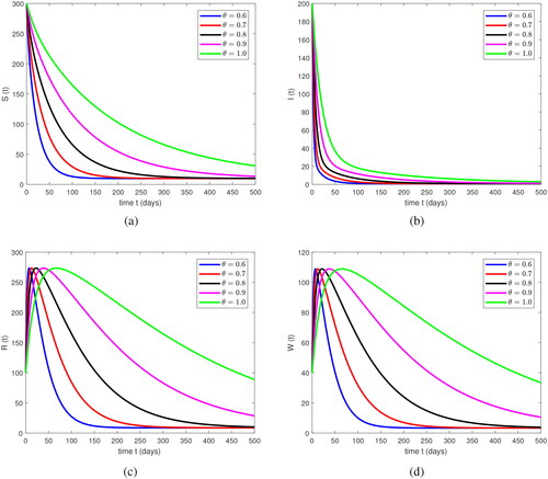
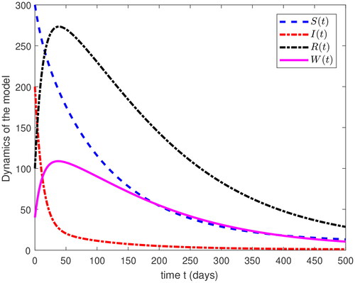
Figure 2. Combine plots of each class in our fractional coronavirus model (3)(3) $$\{\begin{array}{cc}{}^{\mathcal{A}\mathcal{B}\mathcal{C}}{\mathbb{D}}_t^{\theta }(\mathbf{S}(t))\hfill & ={\Pi }^{*}-({\beta }_1^{*}{\mathbf{I}}_h(t)+{\beta }_2^{*}\mathbf{W}(t)+d^{*}){\mathbf{S}}_h(t),\hfill \\ {}^{\mathcal{A}\mathcal{B}\mathcal{C}}{\mathbb{D}}_t^{\theta }(\mathbf{I}(t))\hfill & =({\beta }_1^{*}{\mathbf{I}}_h(t)+{\beta }_2^{*}\mathbf{W}(t)+d^{*}){\mathbf{S}}_h(t)\hfill \\ \hfill & -({\sigma }^{*}+d^{*}+d_1^{*}){\mathbf{I}}_h(t),\hfill \\ {}^{\mathcal{A}\mathcal{B}\mathcal{C}}{\mathbb{D}}_t^{\theta }(\mathbf{R}(t))\hfill & ={\sigma }^{*}{\mathbf{I}}_h(t)-d^{*}{\mathbf{R}}_h(t),\hfill \\ {}^{\mathcal{A}\mathcal{B}\mathcal{C}}{\mathbb{D}}_t^{\theta }(\mathbf{W}(t))\hfill & ={\alpha }^{*}{\mathbf{I}}_h(t)-{\eta }^{*}\mathbf{W}(t),\hfill \end{array}$$(3) for the iterative series.

In Figure 1, the four compartments have been simulated in $(a)-(d)$ subplots versus time t. Figure (a) represents the susceptible individuals where we can see a quick decay in this class. The results show converging behavior and develop the stability for various random values of θ. The green curve represent the stability of integer order, i.e., θ = 1, as the order of θ decrease to noninteger values, i.e., 0.9, 0.8, 0.7 and 0.6 so all the classes are quickly stable as compared to integer order which are represented by pink, black, red and blue curves, respectively. For the graphical representation, the time scale is in days. Similarly, figure (b) represents the basic results for the infected individuals. As with the susceptible individual, one can see a quick decay in the infected agent at various fractional orders. It also reveal that convergence and stability increase with the passage of time. Figure (c) represents the recovered population at different-order θ. In comparison, figure (a) and (b), show a quick increase at the initial time which shows that most of the people are infected and hospitalized. After some time, the growth curve decreases and shows that preventive steps give a rapid recovery and this compartment becomes stable. Figure (d) is for the reservoir class, which reveals a slight evolution in the beginning and reached the ultimate point with time. The gradual decay in the class can be seen for a short time and the solutions go to stable with the passage of time. From Figure 1, we can see that the four classes of Eq. (3)(3) $$\{\begin{array}{cc}{}^{\mathcal{A}\mathcal{B}\mathcal{C}}{\mathbb{D}}_t^{\theta }(\mathbf{S}(t))\hfill & ={\Pi }^{*}-({\beta }_1^{*}{\mathbf{I}}_h(t)+{\beta }_2^{*}\mathbf{W}(t)+d^{*}){\mathbf{S}}_h(t),\hfill \\ {}^{\mathcal{A}\mathcal{B}\mathcal{C}}{\mathbb{D}}_t^{\theta }(\mathbf{I}(t))\hfill & =({\beta }_1^{*}{\mathbf{I}}_h(t)+{\beta }_2^{*}\mathbf{W}(t)+d^{*}){\mathbf{S}}_h(t)\hfill \\ \hfill & -({\sigma }^{*}+d^{*}+d_1^{*}){\mathbf{I}}_h(t),\hfill \\ {}^{\mathcal{A}\mathcal{B}\mathcal{C}}{\mathbb{D}}_t^{\theta }(\mathbf{R}(t))\hfill & ={\sigma }^{*}{\mathbf{I}}_h(t)-d^{*}{\mathbf{R}}_h(t),\hfill \\ {}^{\mathcal{A}\mathcal{B}\mathcal{C}}{\mathbb{D}}_t^{\theta }(\mathbf{W}(t))\hfill & ={\alpha }^{*}{\mathbf{I}}_h(t)-{\eta }^{*}\mathbf{W}(t),\hfill \end{array}$$(3) at other various fractional orders of θ are very near to each other as compared to those in figure $(a)-(d),$ for the data given above. The numerical comparison is very closed to those in Figure 1, but the plot at each fractional order have a large distance from each other. As we vary the order, the simulations converges to those related to integer order. One can also observe that four classes also show convergence and stability of the proposed model. In Figure 2, the four compartments are plotted for time t, by using the data aforementioned.

5. Conclusion

In this work, we have successfully investigated a fractional model of COVID-19 under the nonsingular and nonlocal kernel $\mathcal{A}\mathcal{B}\mathcal{C}$ derivative operator. The considered model has been studied for the existence and uniqueness of the solution by applying the fixed point theory approach. For stability analysis, we have used the Ulam–Hyers stability approach. By utilizing $(\mathcal{A}\mathcal{B}\mathcal{C})$ derivative operator with Adams–Bashforth scheme, we have simulated numerical results. The given plots have been discussed for various fractional-order $0<\theta \le 1.$ Universal spread motility has been reflected for a particular period. It has been observed that the stability of the model occurs quickly at lower fractional orders. At fractional-order equals to unity, the graphs converges to the integer-order curves. Thus, the considered model is more generalized than the classical model. In future, the proposed model can be studied through various nonlocal operators.

Disclosure statement

No potential conflict of interest was reported by the authors.

Data availability statement

The data that support the findings of this study are available within the article.

References

- Abdeljawad, T., & Baleanu, D. (2016). Discrete fractional differences with nonsingular discrete Mittag-Leffler kernels. Advances in Difference Equations, 2016(1), 232. doi:10.1186/s13662-016-0949-5
- Atangana, A., & Baleanu, D. (2016). New fractional derivatives with non-local and nonsingular kernel: Theory and application to heat transfer model. Thermal Science, 20(2), 763–769. doi:10.2298/TSCI160111018A
- Atangana, A., & Gömez-Aguilar, J. F. (2017). A new derivative with normal distribution kernel: Theory, methods and applications. Physica A: Statistical Mechanics and Its Applications. 476, 1–14. doi:10.1016/j.physa.2017.02.016
- Atangana, A., & Gömez-Aguilar, J. F. (2018a). Fractional derivatives with no-index law property: Application to chaos and statistics. Chaos, Solitons & Fractals, 114, 516–535. doi:10.1016/j.chaos.2018.07.033
- Atangana, A., & Gömez-Aguilar, J. F. (2018b). Numerical approximation of Riemann–Liouville definition of fractional derivative: From Riemann–Liouville to Atangana–Baleanu. Numerical Methods for Partial Differential Equations, 34(5), 1502–1523. doi:10.1002/num.22195
- Bogoch, I. I., Watts, A., Thomas-Bachli, A., Huber, C., Kraemer, M. U. G., & Khan, K. (2020). Pneumonia of unknown etiology in Wuhan, China: Potential for international spread via commercial air travel. Journal of Travel Medicine, 27(2), taaa008. doi:10.1093/jtm/taaa008
- Brauer, F., & Castillo-Chavez, C. (2001). Mathematical Models in Population Biology and Epidemiology. In Texts in Applied Math, Vol. 40. Newyork: Springer.
- Cao, J., Xia, J., & Zhao, B. (2020). Mathematical modeling and epidemic prediction of COVID-19 and its significance to epidemic prevention and control measures. Journal of Biomedical Research & Innovation, 1(1), 1–19.
- Caputo, M. (1967). Linear model of dissipation whose Q is almost frequency independent II. Geophysical Journal International, 13(5), 529–539. doi:10.1111/j.1365-246X.1967.tb02303.x
- Caputo, M., & Fabrizio, M. (2015). A new definition of fractional derivative without singular kernel. Progress in Fractional Differentiation and Applications, 1, 73–85.
- Chen, T. M., Rui, J., Wang, Q. P., Zhao, Z. Y., Cui, J. A., & Yin, L. (2020). A mathematical model for simulating the phase-based transmissibility of a novel coronavirus. Infectious Diseases of Poverty, 9(1), 24–28. doi:10.1186/s40249-020-00640-3
- Chowell, G., Fenimore, P. W., & Castillo-Garsow, M. A. (2003). SARS outbreak in Ontario Hong Kong and Singapore: The role of diagnosis and isolation as a control mechanism, Los Alamos Unclassified Report LA-UR-03-2653.
- Dokuyucu, M. A., Celik, E., Bulut, H., & Baskonu, H. M. (2018). Cancer treatment model with the Caputo–Fabrizio fractional derivative. The European Physical Journal Plus, 133, 1–6.
- Furati, K. M., Kassim, M. D., & Tatar, N. T. (2012). Existence and uniqueness for a problem involving Hilfer fractional derivative. Computers & Mathematics with Applications. 64(6), 1616–1626. doi:10.1016/j.camwa.2012.01.009
- He, J. H. (2014). A tutorial review on fractal spacetime and fractional calculus. International Journal of Theoretical Physics, 53(11), 3698–3718. doi:10.1007/s10773-014-2123-8
- He, J. H. (2018). Fractal calculus and its geometrical explanation. Results in Physics, 10, 272–276. doi:10.1016/j.rinp.2018.06.011
- He, J. H., & Ain, Q. T. (2020). New promises and future challenges of fractal calculus: From two-scale thermodynamics to fractal variational principle. Thermal Science, 24(2 Part A), 659–681. doi:10.2298/TSCI200127065H
- He, J. H., Elagan, S. K., & Li, Z. B. (2012). Geometrical explanation of the fractional complex transform and derivative chain rule for fractional calculus. Physics Letters A, 376(4), 257–259. doi:10.1016/j.physleta.2011.11.030
- He, J. H., & El-Dib, Y. O. (2020). Periodic property of the time-fractional Kundu–Mukherjee–Naskar equation. Results in Physics, 19, 103345. doi:10.1016/j.rinp.2020.103345
- He, J. H., Qie, N., & He, C. H. (2021). Solitary waves travelling along an unsmooth boundary. Results in Physics, 24, 104104. doi:10.1016/j.rinp.2021.104104
- Huang, C., Wang, Y., Li, X., Ren, L., Zhao, J., Hu, Y., … Cao, B. (2020). Clinical features of patients infected with 2019 novel coronavirus in Wuhan, China. Lancet (London, England), 395(10223), 497–506. doi:10.1016/S0140-6736(20)30183-5
- Hui, D. S., I Azhar, E., Madani, T. A., Ntoumi, F., Kock, R., Dar, O., … Petersen, E. (2020). The continuing 2019-nCoV epidemic threat of novel coronaviruses to global health–the latest 2019 Novel coronavirus outbreak in Wuhan. China. International Journal of Infectious Diseases, 91(2020), 264–266. doi:10.1016/j.ijid.2020.01.009
- Ivorra, B., Ferrández, M. R., Vela-Pérez, M., & Ramos, A. M. (2020). Mathematical modeling of the spread of the coronavirus disease 2019 (COVID-19) taking into account the undetected infections. The case of China. Communications in Nonlinear Science & Numerical Simulation, 88, 105303. doi:10.1016/j.cnsns.2020.105303
- Jarad, F., Abdeljawad, T., & Hammouch, Z. (2018). On a class of ordinary differential equations in the frame of Atangana-Baleanu fractional derivative. Chaos Solitons & Fractals, 117, 16–20. doi:10.1016/j.chaos.2018.10.006
- Jung, S. M., Akhmetzhanov, A. R., Katsuma, H., Linton, N. M., Yang, Y., Yuan, B., … Nishiura, H. (2020). Real-time estimation of the risk of death from novel coronavirus (COVID-19) infection: Inference using exported cases. Journal of Clinical Medicine, 9(2), 523. doi:10.3390/jcm9020523
- Khan, H., Li, Y., Khan, A., & Khan, A. (2019). Existence of solution for a fractional-order Lotka-Volterra reaction-diffusion model with Mittag-Leffler kernel. Mathematical Methods in the Applied Sciences, 42(9), 3377–3387. doi:10.1002/mma.5590
- Khan, T., Zaman, G., Foong, O. M., Fatima, B., Khan, I., & Nisar, K. S. (2020). Modeling and control of the Novel Coronavirus (COVID-19). Computer materials and Continua.
- Kilbas, A. A., Marechiv, O. I., & Samko, S. G. (1993). Fractional integrals and derivatives, (Theory and applications). Minsk; Nauka I Tekhnika. Switzerland: Gordon and Breach.
- Kilbas, A. A., Srivastava, H. M., & Trujillo, J. J. (2006). Theory and applications of fractional differential equations (Vol. 204). Amsterdam; Boston: Elsevier.
- Kumar, S., Ahmadian, A., Kumar, R., Kumar, D., Singh, J., Baleanu, D., & Salimi, M. (2020). An efficient numerical method for fractional SIR epidemic model of infectious disease by using Bernstein wavelets. Mathematics, 8(4), 558. doi:10.3390/math8040558
- Kumar, S., Chauhan, R. P., Momani, S., & Hadid, S. (2020). Numerical investigations on COVID-19 model through singular and non-singular fractional operators. Numerical Methods for Partial Differential Equations. doi:10.1002/num.22707
- Kumar, S., Kumar, R., Agarwal, R. P., & Samet, B. (2020). A study of fractional Lotka-Volterra population model using Haar wavelet and Adams-Bashforth-Moulton methods. Mathematical Methods in the Applied Sciences, 43(8), 5564–5578. doi:10.1002/mma.6297
- Kumar, S., Kumar, R., Cattani, C., & Samet, B. (2020). Chaotic behaviour of fractional predator-prey dynamical system. Chaos, Solitons & Fractals, 135, 109811. doi:10.1016/j.chaos.2020.109811
- Kumar, S., Kumar, R., Momani, S., & Hadid, S. (2021). A study on fractional COVID-19 disease model by using Hermite wavelets. Mathematicsl Methods in the Applied Sciences. doi: 10.1002/mma.7065
- Li, Q., Guan, X., Wu, P., Wang, X., Zhou, L., Tong, Y., … Feng, Z. (2020). Early transmission dynamics in Wuhan, China, of novel coronavirus-infected pneumonia. The New England Journal of Medicine, 382(13), 1199–1207. doi:10.1056/NEJMoa2001316
- Lin, Q., Zhao, S., Gao, D., Lou, Y., Yang, S., Musa, S. S., … He, D. (2020). A conceptual model for the coronavirus disease 2019 (COVID-19) outbreak in Wuhan, China with individual reaction and governmental action. International Journal of Infectious Diseases, 93, 211–216. doi:10.1016/j.ijid.2020.02.058
- Ma, Z. S. (2020). A simple mathematical model for estimating the inflection points of COVID-19 outbreaks. medRxiv. doi:10.1101/2020.03.25.20043893
- Maier, B. F., & Brockmann, D. (2020). Effective containment explains subexponential growth in recent confirmed COVID-19 cases in China. Science (New York, N.Y.), 368(6492), 742–746. doi:10.1126/science.abb4557
- Martcheva, M. (2015). An introduction to mathematical epidemiology. New York: Springer.
- Michael, S. (2020). Rosenwald, History’s deadliest pandemics, from ancient Rome to modern America. The Washington Post. Archived from the original on 7 April 2020.
- Miller, S. K., & Ross, B. (1993). An introduction to the fractional calculus and fractional differential equations. New York: Wiley.
- National Centre for Disease Control. (2020a). Travel Advisory. Retrieved from https://ncdc.gov.in/WriteReadData/l892s/63950984511580999086.pdf
- National Centre for Disease Control. (2020b). COVID-19 outbreak in China–travel advisory to travelers visiting China. Retrieved from https://ncdc.gov.in/WriteReadData/l892s/34827556791580715701.pdf
- Omay, T., & Baleanu, D. (2021). Fractional unit-root tests allowing for a fractional frequency flexible Fourier form trend: Predictability of COVID-19. Advances in Difference Equations, 2021(1), 1–33. doi:10.1186/s13662-021-03317-9
- Peter, O. J., Shaikh, A. S., Ibrahim, M. O., Nisar, K. S., Baleanu, D., Khan, I., & Abioye, A. I. (2021). Analysis and dynamics of fractional order mathematical model of COVID-19 in Nigeria using Atangana-Baleanu operator. Computers, Materials & Continua, 66(2), 1823–1848. doi:10.32604/cmc.2020.012314
- Qu, H., Liu, X., Lu, X., Ur Rahman, M., & She, Z. (2022). Neural network method for solving nonlinear fractional advection-diffusion equation with spatiotemporal variable-order. Chaos, Solitons & Fractals, 156, 111856. doi:10.1016/j.chaos.2022.111856
- Social Distancing, Quarantine, and Isolation-CDC (2020). Retrieved from www.cdc.gov
- Sweilam, N. H., Al-Mekhlafi, S. M., & Baleanu, D. (2021). A hybrid stochastic fractional order Coronavirus (2019-nCov) mathematical model. Chaos, Solitons, and Fractals, 145, 110762. doi:10.1016/j.chaos.2021.110762
- Toufik, M., & Atangana, A. (2017). New numerical approximation of fractional derivative with non-local and non-singular kernel: Application to chaotic models. The European Physical Journal plus, 132(10), 444. doi:10.1140/epjp/i2017-11717-0
- Trilla, A. (2020). One world, one health: The novel coronavirus COVID-19 epidemic. Medicina Clinica (English ed.), 154(5), 175–177. doi:10.1016/j.medcle.2020.02.001
- Veeresha, P., Prakasha, D. G., & Baskonus, H. M. (2019). New numerical surfaces to the mathematical model of cancer chemotherapy effect in Caputo fractional derivatives. Chaos (Woodbury, N.Y.), 29(1), 013119. doi:10.1063/1.5074099
- Veeresha, P., Prakasha, D. G., & Kumar, S. (2020). A fractional model for propagation of classical optical solitons by using nonsingular derivative. Mathematics Methods in the Applied Sciences. doi:10.1002/mma.6335
- Wang, K. L., Wang, K. J., & He, C. H. (2019). Physical insight of local fractional calculus and its application to fractional Kdv–Burgers–Kuramoto equation. Fractals, 27(07), 1950122. doi:10.1142/S0218348X19501226
- Wong, G., Liu, W., Liu, Y., Zhou, B., Bi, Y., & Gao, G. F. (2015). MERS, SARS, and Ebola: The role of super-spreaders in infectious disease. Cell Host & Microbe, 18(4), 398–401. doi:10.1016/j.chom.2015.09.013
- World Health Organization. (2020a). Pneumonia of unknown cause–China. Retrieved from www.who.int/csr/don/05-january-2020-pneumonia-of-unkown-cause-China/en/
- World Health Organization. (2020b). Updated WHO advice for international traffic in relation to the outbreak of the COVID-19. WHO, Geneva. Retrieved from https://www.who.int/ith/COVID-19adviceforinternationaltraffic/en/
- Worldometer. (2020). COVID-19 coronavirus pandemic. Retrieved from https://www.worldometers.info/coronavirus
- Wu, J. T., Leung, K., & Leung, G. M. (2020). Now casting and fore casting the potential domestic and international spread of the 2019-nCoV outbreak originating in Wuhan, China: A modelling study. The Lancet, 395(10225), 689–697.
- Xu, C., Liao, M., Li, P., & Yuan, S. (2021). Impact of leakage delay on bifurcation in fractional-order complex-valued neural networks. Chaos, Solitons & Fractals, 142, 110535. doi:10.1016/j.chaos.2020.110535
- Zhang, L., Ur Rahman, M., Arfan, M., & Ali, A. (2021). Investigation of mathematical model of transmission co-infection TB in HIV community with a non-singular kernel. Results in Physics, 28, 104559. doi:10.1016/j.rinp.2021.104559