A new technique for solving regular and singular coupled Burgers’ equation

Abstract

The primary objective of this research paper is to introduce a novel technique known as the double ARA transform (DARAT) for effectively solving a broad spectrum of problems, encompassing both linear and nonlinear scenarios. This study specifically explores the application of DARAT to address the regular and singular one-dimensional coupled Burgers’ equations. Significant enhancements have been made to the original ARA transform to improve its precision and accuracy in handling linear problems. Additionally, DARAT has been seamlessly integrated with the well-established Adomian decomposition technique, which is renowned for its efficacy in solving nonlinear issues. The effectiveness of our proposed method is demonstrated through its remarkable ability to solve partial differential equations (PDEs), with the results clearly illustrated through graphical representations and detailed tables. These outcomes affirm the method’s robustness in deriving accurate solutions for both regular and singular coupled Burgers’ equations.

Keywords:

• ARA transform
• double ARA transform
• double convolution theorem
• partial differential equations

1. Introduction

Integral transform methods are foundational and broadly employed in solving partial differential equations (PDEs). These equations are critical for modeling a vast array of phenomena across various disciplines related to mathematics, such as physics, engineering, and other scientific fields. These models are articulated through diverse PDEs as referenced in studies by (Alam & Tunc, 2016; Alam & Tunç, 2020; Eddine & Ragusa, 2022; Constanda, 2018; Evans, 2010; Islam, Alam, Fayz-Al-Asad, & Tunç, 2021; A. K. H. Sedeeg, 2023).

Integral transforms are similarly effective in resolving PDEs. This study primarily employs the double ARA transform to tackle these equations. This double integral transform offers a potent tool, transforming PDEs into algebraic equations that facilitate the derivation of exact solutions. This research builds on significant advancements by scholars who have dedicated substantial effort to develop and apply these methods across a broad spectrum of mathematical challenges. Notable examples include the double Laplace transform (R. R. Dhunde, Bhondge, & Dhongle, 2013; R. Dhunde & Waghmare, 2017; Eltayeb & Kilicman, 2010; Eltayeb & Kiliçman, 2013; Eshag, 2017), the double Laplace-Sumudu transform (S. A. Ahmed, Elzaki, & Hassan, 2020), the double Sumudu transform (Z. Ahmed, Idrees, Belgacem, & Perveen, 2019; Al-Omari, 2012; Eltayeb & Kilicman, 2010; Tchuenche & Mbare, 2007), the double Laplace-ARA transform(A. K. Sedeeg, Mahamoud, & Saadeh, 2022), the double ARA - Sumudu transform (Qazza, Burqan, Saadeh, & Khalil, 2022; Saadeh, Qazza, & Burqan, 2022), the double Elzaki transform (Idrees, Ahmed, Awais, & Perveen, 2018), the double Kamal transform (Sonawane & Kiwne, 2019), the double Shehu transform (Alfaqeih & Misirli, 2020), among others.

More recently, Saadeh et al (Saadeh, Qazza, & Burqan, 2020) introduced an innovative integral transform termed the ARA transform, formulated as follows: (1.1) $${\mathcal{G}}_n\left[h\left(x\right)\right]=Q\left(n,r\right)=r{\int }_0^{\mathrm{\infty }}{x}^{n-1}{e}^{-\mathit{\text{rx}}}h\left(x\right)\mathit{\text{dx}},\hspace{0.5em}r>0.$$(1.1)

The name "ARA" uniquely identifies this transform and is not an abbreviation. One of its distinctive properties is the ability to generate various integral transforms by altering the value of $n.$ Additionally, as highlighted in Saadeh et al. (2020), this transform effectively circumvents the singularity at $x=0,$ presenting a significant advantage for mathematical applications. Extensive research has been dedicated to the development and application of this transform; for instance, it has been applied by Saadeh et al (Burqan et al., 2021; Qazza, Burqan, & Saadeh, 2021) in solving complex fractional differential equations and fractional neutral pantograph equations. Furthermore, Abdelilah and colleagues have combined the ARA transform with the Laplace transform (A. K. Sedeeg et al., 2022) to address partial differential equations, and it has been integrated with the Sumudu transform by Qazza et al as well as Saadeh et al to tackle both integral and fractional equations effetively (Qazza et al., 2022; Saadeh et al., 2022). In a more recent study, Saadeh and colleagues (Saadeh, Sedeeg, Amleh, & Mahamoud, 2023) innovatively merged the ARA transform with the Laplace and Sumudu transforms to solve multi-variable partial differential equations, thereby confirming its efficacy as a tool for solving linear partial differential and integral equations.

Given the robust capabilities highlighted previously, we have adopted the new double ARA transform to solve both the regular and singular one-dimensional coupled Burgers’ equations. This work introduces an innovative analytical method, the DARAT, combined with the Adomian decomposition technique, providing the scientific community with a potent and reliable tool for addressing a broad spectrum of linear and nonlinear problems within the realm of partial differential equations (PDEs). The effectiveness of this approach is demonstrated through the graphical and tabulated solutions included in this paper, which not only underscore the method’s efficacy but also solidify its value as a significant asset in mathematical modeling and analysis. Although primarily yielding approximate numerical solutions that rapidly converge towards exact solutions, it’s important to note that there are certain limitations related to the conditions under which the method can be applied effectively.

The objective of this paper is to propose an analytical solution for one-dimensional regular and singular coupled Burgers’ equations using the double ARA decomposition method (DARADM), as referenced by (Eltayeb, Bachar, & Kılıçman, 2019; Mohamed, Hamza, & Sedeeg, 2023; Nee & Duan, 1998; Younis, Zafar, Ul-Haq, & Rahman, 2013). The coupled Burgers’ equations addressed are expressed as belows: (1.2) $$\begin{array}{c}\frac{\partial \zeta (x,t)}{\partial t}-\frac{{\partial }^2\zeta (x,t)}{\partial x^2}+\lambda \mathrm{ }\zeta (x,t)\frac{\partial \zeta (x,t)}{\partial x}+\alpha \mathrm{ }\frac{\partial }{\partial x}\left(\zeta (x,t)\xi (x,t)\right)=u\left(x,t\right)\\ \frac{\partial \xi (x,t)}{\partial t}-\frac{{\partial }^2\xi (x,t)}{\partial x^2}+\lambda \mathrm{ }\xi (x,t)\frac{\partial \xi (x,t)}{\partial x}+\beta \mathrm{ }\frac{\partial }{\partial x}\left(\zeta (x,t)\xi (x,t)\right)=v\left(x,t\right)\end{array},\hspace{0.5em}t>0,$$(1.2)

subject to (1.3) $$\zeta \left(x,0\right)=u_1\left(x\right),\hspace{0.5em}\xi \left(x,0\right)=v_1\left(x\right),$$(1.3) where $\zeta \left(x,t\right)$ and $\xi \left(x,t\right)$ are unknown functions, $u\left(x,t\right),v\left(x,t\right),u_1\left(x\right)$ and $v_1\left(x\right)$ are given functions, $\lambda ,\alpha$ and $\beta$ are parameters depend on the system characteristics such as Peclet number, Stokes velocity of particles due to gravity, and Brownian diffusivity.

Burgers’ equation serves as a potent model for various mathematical challenges, particularly in the context of fluid dynamics where phenomena such as shocks or viscous dissipation play crucial roles. The equation’s analytical solutions were first explored by Bateman in 1915. Named after Jan Burgers, who began his seminal work in 1939 and published in 1948, Burgers’ equation has been a fundamental tool in modeling turbulence and a myriad of other physical phenomena. These include, but are not limited to, shock flows, traffic flow, and acoustic transmission through fog. The significance of this equation extends across physics and other sciences, prompting ongoing research into its applications in modeling natural and biological phenomena, particularly in their fractional forms. Notably, Burgers’ equation has been applied in simple models of traffic flow, introduced independently by Lighthill-Whitham and Richards, and in coagulation theory. Its nonlinear nature makes it a valuable prototype for modeling diverse and seemingly unrelated phenomena such as shock flows, wave propagation in combustion chambers, vehicular traffic, and acoustic transmission.

This article is structured as follows: Section 2 outlines some fundamental aspects of the single ARA transformation of order one. Section 3 introduces the new double ARA integral transform and discusses some of its properties. Sections 4 and 5 apply the double ARA decomposition method to the one-dimensional Burgers’ equation, both in its singular and regular coupled forms. Section 6 presents three case studies where the double ARA decomposition method (DARADM) is applied. Finally, Sections 7 and 8 contain discussions of the results and conclusions of this study.

2. Facts and properties of single ARA transform of order one (Saadeh et al., 2020)

In this section we introduce the definition and basic facts about single ARA transform of order one.

Definition 2.1.

The ARA transformation of order one of piecewise continuous function $h(x)$ on $0\le x\le \mathrm{\infty }$ is express by (2.1) $${\mathcal{G}}_1\left[h\left(x\right)\right]=H\left(r\right)=r{\int }_0^{\mathrm{\infty }}{e}^{-\mathit{\text{rx}}}h\left(x\right)\mathit{\text{dx}},r>0.$$(2.1)

For simplicity, let us denote ${\mathcal{G}}_1\left[h\left(x\right)\right]$ by $\mathcal{G}\left[h\left(x\right)\right].$

Thus, the inverse single ARA transform is expressed as (2.2) $${\mathcal{G}}^{-1}\left[\mathrm{H}\left(r\right)\right]=\frac{1}{2\mathrm{\pi i}}{\int }_{z-i\mathrm{\infty }}^{z+i\mathrm{\infty }}\frac{e^{\mathit{\text{rx}}}}{r}\left[\mathrm{H}\left(r\right)\right]\mathit{\text{dr}}=h\left(x\right),z\in \mathcal{R}.$$(2.2)

The below theorem shows the existence condition for single ARA integral transform Equation (2.1)(2.1) $${\mathcal{G}}_1\left[h\left(x\right)\right]=H\left(r\right)=r{\int }_0^{\mathrm{\infty }}{e}^{-\mathit{\text{rx}}}h\left(x\right)\mathit{\text{dx}},r>0.$$(2.1) .

Theorem 2.1.

(Existence conditions). Let $h(x)$ be exponential order bounded by $M{e}^{\mathrm{\alpha x}}$ and piecewise continuous on $0\le x\le \mathrm{\infty },$ then $\mathcal{G}\left[h\right(x\left)\right]$ exists for $\mathit{\text{Re}}(r)>\alpha$ and satisfies: (2.3) $$\left|h\left(x\right)\right|\le M{e}^{\mathrm{\alpha x}},$$(2.3) where $M$ is a positive constant.

In the following, we state some basic properties of single ARA transform.

Assume that $H(r)=\mathcal{G}\left[h\left(x\right)\right]$ and $G\left(r\right)=\mathcal{G}\left[g\left(x\right)\right]$ and $a,b\in \mathcal{R}.$ Then: (2.4) $$\mathcal{G}\left[a\mathrm{ }h\left(x\right)+b\mathrm{ }g\left(x\right)\right]=a\mathrm{ }\mathcal{G}\left[h\left(x\right)\right]+b\mathrm{ }\mathcal{G}\left[g\left(x\right)\right].$$(2.4) (2.5) $${\mathcal{G}}^{-1}\left[a\mathrm{ }H\left(r\right)+b\mathrm{ }G\left(r\right)\right]=a\mathrm{ }{\mathcal{G}}^{-1}\left[H\left(r\right)\right]+b\mathrm{ }{\mathcal{G}}^{-1}\left[G\left(r\right)\right].$$(2.5) (2.6) $$\mathcal{G}\left[x^{\alpha }\right]=\frac{\alpha !}{r^{\alpha }},\alpha \ge 0.$$(2.6) (2.7) $$\mathcal{G}\left[e^{\mathit{\text{ax}}}\right]=\frac{r}{r-a}.$$(2.7) (2.8) $$\mathcal{G}\left[\mathrm{\text{sin}}\hspace{0.17em}\mathit{\text{ax}}\right]=\frac{\mathit{\text{ar}}}{r^2+a^2}.$$(2.8) (2.9) $$\mathcal{G}\left[\mathrm{\text{cos}}\hspace{0.17em}\mathit{\text{ax}}\right]=\frac{r^2}{r^2+a^2}.$$(2.9) (2.10) $$\mathcal{G}\left[\mathrm{\text{sinh}}\hspace{0.17em}\mathit{\text{ax}}\right]=\frac{\mathit{\text{ar}}}{r^2-a^2}.$$(2.10) (2.11) $$\mathcal{G}\left[\mathrm{\text{cosh}}\hspace{0.17em}\mathit{\text{ax}}\right]=\frac{r^2}{r^2-a^2}.$$(2.11) (2.12) $$\mathcal{G}\left[h^{\left(n\right)}\left(x\right)\right]=r^n\mathcal{G}\left[h\left(x\right)\right]-\sum _{k=1}^n{r}^{n-k+1}{h}^{\left(k-1\right)}\left(0\right).$$(2.12)

The above results can be obtained from the definition of single ARA transforms and simple calculations.

3. Double ARA transform of order one (DARAT)

In this section, a new integral transform, DARAT. We present basic properties concerning the existence conditions, linearity, and the inverse of this transform. Moreover, some essential properties and results are used to compute the DARAT for some basic functions. We introduce the convolution theorem and the derivatives properties of the new transform.

Definition 3.1.

Let $\zeta (x,t)$ be continuous function of two positive variables $x$ and $t.$ Then the DARAT of $\zeta (x,t)$ is defined as (3.1) $${\mathcal{G}}_x{\mathcal{G}}_t\left[\zeta \left(x,t\right)\right]=\mathrm{\Phi }\left(r,s\right)=\mathit{\text{rs}}{\int }_0^{\mathrm{\infty }}{\int }_0^{\mathrm{\infty }}{e}^{-\left(\mathit{\text{rx}}+\mathit{\text{st}}\right)}\left[\zeta \left(x,t\right)\right]d\mathit{\text{xdt}},r,s>0,$$(3.1) provided the integral exists.

Clearly, the DARAT is a linear integral transformation as shown below. $$\begin{array}{c}{\mathcal{G}}_x{\mathcal{G}}_t\left[A\mathrm{ }\zeta \left(x,t\right)+B\mathrm{ }\xi (x,t)\right]=\mathit{\text{rs}}{\int }_0^{\mathrm{\infty }}{\int }_0^{\mathrm{\infty }}{e}^{-\left(\mathit{\text{rx}}+\mathit{\text{st}}\right)}\left[A\mathrm{ }\zeta \left(x,t\right)+B\mathrm{ }\xi (x,t)\right]d\mathit{\text{xdt}}\\ =\mathit{\text{rA}}{\int }_0^{\mathrm{\infty }}{\int }_0^{\mathrm{\infty }}{e}^{-\left(\mathit{\text{rx}}+\mathit{\text{st}}\right)}\left[\zeta \left(x,t\right)\right]d\mathit{\text{xdt}}+s\mathrm{ }B{\int }_0^{\mathrm{\infty }}{\int }_0^{\mathrm{\infty }}{e}^{-\left(\mathit{\text{rx}}+\mathit{\text{st}}\right)}\left[\xi (x,t)\right]d\mathit{\text{xdt}}\\ =A\mathrm{ }{\mathcal{G}}_x{\mathcal{G}}_t\left[\mathrm{ }\zeta \left(x,t\right)\right]+\mathrm{B}\mathrm{ }{\mathcal{G}}_x{\mathcal{G}}_t\left[\xi (x,t)\right],\end{array}$$ where $A$ and $B$ are constants and ${\mathcal{G}}_x{\mathcal{G}}_t\left[\zeta \left(x,t\right)\right]$ and ${\mathcal{G}}_x{\mathcal{G}}_t\left[\xi (x,t)\right]$ exists and the inverse of the DARAT is given by: (3.2) $${\mathcal{G}}_r^{-1}\left[{\mathcal{G}}_s^{-1}\left[\mathrm{\Phi }\left(r,s\right)\right]\right]=\left(\frac{1}{2\mathrm{\pi i}}\right){\int }_{c-i\mathrm{\infty }}^{c+i\mathrm{\infty }}\frac{e^{\mathit{\text{rx}}}}{r}\mathit{\text{dr}}\left(\frac{1}{2\mathrm{\pi i}}\right){\int }_{d-i\mathrm{\infty }}^{d+i\mathrm{\infty }}\frac{e^{\mathit{\text{st}}}}{s}\mathrm{\Phi }\left(r,s\right)\mathit{\text{ds}}=\zeta \left(x,t\right),c,d\in \mathcal{R}.$$(3.2)

In addition, Abdelilah and others, during their previous study, found that the relationship between the DL-ARA and the DARAT transforms is that the defined operator is a constant multiple of the operator defined in Sedeeg et al. (2022).

Property 3.1.

Let $\zeta \left(x,t\right)=f\left(x\right)g\left(t\right),x>0\mathrm{ }$ and $t>0.$ Then: $${\mathcal{G}}_x{\mathcal{G}}_t\left[\zeta (x,t)\right]={\mathcal{G}}_x\left[f\left(x\right)\right]{\mathcal{G}}_t\left[g\left(t\right)\right].$$

Proof of Property 3.1.

Using the definition of ARA transform, we get $$\begin{array}{c}{{\mathcal{G}}_x{\mathcal{G}}_t\left[\zeta (x,t)\right]=\mathcal{G}}_x{\mathcal{G}}_t\left[f\left(x\right)g\left(t\right)\right]=\mathit{\text{rs}}{\int }_0^{\mathrm{\infty }}{\int }_0^{\mathrm{\infty }}{e}^{-\left(\mathit{\text{rx}}+\mathit{\text{st}}\right)}\left[f\left(x\right)g\left(t\right)\right]d\mathit{\text{xdt}}\\ =r{\int }_0^{\mathrm{\infty }}f\left(x\right)e^{-\mathit{\text{rx}}}\mathit{\text{dx}}\mathrm{ }s{\int }_0^{\mathrm{\infty }}{g\left(t\right)e}^{-\mathit{\text{st}}}\mathit{\text{dt}}={\mathcal{G}}_x\left[f\left(x\right)\right]{\mathcal{G}}_t\left[g\left(t\right)\right].\end{array}$$

3.1. Double ARA transform of some elementary functions

In the following arguments, we introduce the Double ARA Transform for some basic functions.

1. Let $\zeta \left(x,t\right)=1,x>0\mathrm{ }$ and $t>0.$ Then $${\mathcal{G}}_x{\mathcal{G}}_t\left[1\right]=\mathit{\text{rs}}{\int }_0^{\mathrm{\infty }}{\int }_0^{\mathrm{\infty }}{e}^{-(\mathit{\text{rx}}+\mathit{\text{st}})}d\mathit{\text{xdt}}=r{\int }_0^{\mathrm{\infty }}{e}^{-\mathit{\text{rx}}}\mathit{\text{dx.}}s{\int }_0^{\mathrm{\infty }}{e}^{-\mathit{\text{st}}}\mathit{\text{dt}},$$ from Property 3.1. and Equation (2.6)(2.6) $$\mathcal{G}\left[x^{\alpha }\right]=\frac{\alpha !}{r^{\alpha }},\alpha \ge 0.$$(2.6) , we get $${\mathcal{G}}_x{\mathcal{G}}_t\left[1\right]={\mathcal{G}}_x\left[1\right]{\mathcal{G}}_t\left[1\right]=1.$$

1. Let $\zeta \left(x,t\right)=x^{\alpha }{t}^{\beta },x>0,t>0\mathrm{ }$ and $\alpha ,\beta$ are constants. Then $${\mathcal{G}}_x{\mathcal{G}}_t\left[x^{\alpha }{t}^{\beta }\right]=\mathit{\text{rs}}{\int }_0^{\mathrm{\infty }}{\int }_0^{\mathrm{\infty }}{e}^{-\left(\mathit{\text{rx}}+\mathit{\text{st}}\right)}\left[x^{\alpha }{t}^{\beta }\right]d\mathit{\text{xdt}}=r{\int }_0^{\mathrm{\infty }}{e}^{-\mathit{\text{rx}}}\left[x^{\alpha }\right]\mathit{\text{dx}}\bullet s{\int }_0^{\mathrm{\infty }}{e}^{-\mathit{\text{st}}}\left[t^{\beta }\right]\mathit{\text{dt}},$$ from Property 3.1 and Equation (2.6)(2.6) $$\mathcal{G}\left[x^{\alpha }\right]=\frac{\alpha !}{r^{\alpha }},\alpha \ge 0.$$(2.6) , we get $${{\mathcal{G}}_x{\mathcal{G}}_t\left[x^{\alpha }{t}^{\beta }\right]=\mathcal{G}}_x\left[x^{\alpha }\right]{\mathcal{G}}_t\left[t^{\beta }\right]=\frac{\alpha !}{r^{\alpha }}\frac{\beta !}{s^{\beta }}.$$

1. Let $\zeta \left(x,t\right)=e^{\mathrm{\alpha x}+\mathrm{\beta t}},x>0,t>0$ and $\alpha ,\beta$ are constants. Then $${\mathcal{G}}_x{\mathcal{G}}_t\left[e^{\mathrm{\alpha x}+\mathrm{\beta t}}\right]=\mathit{\text{rs}}{\int }_0^{\mathrm{\infty }}{\int }_0^{\mathrm{\infty }}{e}^{-(\mathit{\text{rx}}+\mathit{\text{st}})}\left[e^{\mathrm{\alpha x}+\mathrm{\beta t}}\right]d\mathit{\text{xdt}}=r{\int }_0^{\mathrm{\infty }}{e}^{-\mathit{\text{rx}}}\left[e^{\mathrm{\alpha x}}\right]\mathit{\text{dx·}}s{\int }_0^{\mathrm{\infty }}{e}^{-\mathit{\text{st}}}\left[e^{\mathrm{\beta t}}\right]\mathit{\text{dt}},$$

from Property 3.1 and Eq. (2.7)(2.7) $$\mathcal{G}\left[e^{\mathit{\text{ax}}}\right]=\frac{r}{r-a}.$$(2.7) , we get $${\mathcal{G}}_x{\mathcal{G}}_t\left[e^{\mathrm{\alpha x}+\mathrm{\beta t}}\right]={\mathcal{G}}_x\left[e^{\mathrm{\alpha x}}\right]{\mathcal{G}}_t\left[e^{\mathrm{\beta t}}\right]=\frac{\mathit{\text{rs}}}{\left(r-\alpha \right)\left(s-\beta \right)}.$$

Similarly, $${\mathcal{G}}_x{\mathcal{G}}_t\left[e^{i\left(\mathrm{\alpha x}+\mathrm{\beta t}\right)}\right]=\frac{\mathit{\text{rs}}}{\left(r-\mathrm{i\alpha }\right)\left(s-\mathrm{i\beta }\right)}.$$

Using the property of complex analysis, we have $${\mathcal{G}}_x{\mathcal{G}}_t\left[e^{i\left(\mathrm{\alpha x}+\mathrm{\beta t}\right)}\right]=\frac{\mathit{\text{rs}}\left(\mathit{\text{rs}}-\mathrm{\alpha \beta }\right)+\mathit{\text{irs}}(\mathrm{r\beta }+\mathrm{s\alpha })}{\left(r^2+{\alpha }^2\right)\left(s^2+{\beta }^2\right)}.$$

Using Euler’s formulas $\mathrm{\text{sin}}\hspace{0.17em}x=\frac{e^{\mathit{\text{ix}}}-e^{-\mathit{\text{ix}}}}{2i}$ and $\mathrm{\text{cos}}\hspace{0.17em}x=\frac{e^{\mathit{\text{ix}}}+e^{-\mathit{\text{ix}}}}{2},$ and the formulas $\mathrm{\text{sinh}}\hspace{0.17em}x=\frac{e^x-e^{-x}}{2}$ and $\mathrm{\text{cosh}}\hspace{0.17em}x=\frac{e^x+e^{-x}}{2}.$

Now, we find the DARAT of the following functions. $${\mathcal{G}}_x{\mathcal{G}}_t\left[\mathrm{\text{sin}}\hspace{0.17em}\left(\mathrm{\alpha x}+\mathrm{\beta t}\right)\right]=\frac{\mathit{\text{rs}}(\mathrm{r\beta }+\mathrm{s\alpha })}{\left(r^2+{\alpha }^2\right)\left(s^2+{\beta }^2\right)},$$ $${\mathcal{G}}_x{\mathcal{G}}_t\left[\mathrm{\text{cos}}\hspace{0.17em}\left(\mathrm{\alpha x}+\mathrm{\beta t}\right)\right]=\frac{\mathit{\text{rs}}\left(\mathit{\text{sr}}-\mathrm{\alpha \beta }\right)}{\left(r^2+{\alpha }^2\right)\left(s^2+{\beta }^2\right)},$$ $${\mathcal{G}}_x{\mathcal{G}}_t\left[\mathrm{\text{sinh}}\hspace{0.17em}\left(\mathrm{\alpha x}+\mathrm{\beta t}\right)\right]=\frac{\mathit{\text{rs}}(\mathrm{r\beta }+\mathrm{s\alpha })}{\left(r^2-{\alpha }^2\right)\left(s^2-{\beta }^2\right)},$$ $${\mathcal{G}}_x{\mathcal{G}}_t\left[\mathrm{\text{cosh}}\hspace{0.17em}\left(\mathrm{\alpha x}+\mathrm{\beta t}\right)\right]=\frac{\mathit{\text{rs}}\left(\mathit{\text{sr}}+\mathrm{\alpha \beta }\right)}{\left(r^2-{\alpha }^2\right)\left(s^2-{\beta }^2\right)}.$$

1. Let $\mathrm{ }\zeta \left(x,t\right)=J_0\left(\eta \sqrt{\mathit{\text{xt}}}\right),x>0,t>0\mathrm{ }$ and $\mathrm{ }\eta \in \mathcal{R}.$ Then $${\mathcal{G}}_x{\mathcal{G}}_t\left[J_0\left(\eta \sqrt{\mathit{\text{xt}}}\right)\right]=r{\int }_0^{\mathrm{\infty }}{e}^{-\mathit{\text{rx}}}\left[J_0\left(\eta \sqrt{\mathit{\text{xt}}}\right)\right]\mathit{\text{dx}}\bullet s{\int }_0^{\mathrm{\infty }}{e}^{-\mathit{\text{st}}}\mathit{\text{dt}}=s{\int }_0^{\mathrm{\infty }}{e^{-\frac{{\eta }^2}{4r}t}e}^{-\mathit{\text{st}}}\mathit{\text{dt}}=\frac{4\mathit{\text{rs}}}{4\mathit{\text{rs}}+{\eta }^2},$$

where $J_0$ is Bessel function of order zero.

3.2. Existence conditions for double ARA transform

Let $\zeta \left(x,t\right)$ be function of exponential order $\alpha$ and $\beta$ as $x\to \mathrm{\infty }$ and $t\to \mathrm{\infty }.$ If there exists a positive $N$ such that $\forall x>X$ and $t>T,$ we have $$\left|\zeta \left(x,t\right)\right|\le N{e}^{\mathrm{\alpha x}+\mathrm{\beta t}},$$ we can write $\zeta \left(x,t\right)=O\left(e^{\mathrm{\alpha x}+\mathrm{\beta t}}\right)$ as $x\to \mathrm{\infty },t\to \mathrm{\infty },$ $r>\alpha$ and $s>\beta .$

The below theorem shows the existence condition for double ARA integral transform Eq.(3.1)(3.1) $${\mathcal{G}}_x{\mathcal{G}}_t\left[\zeta \left(x,t\right)\right]=\mathrm{\Phi }\left(r,s\right)=\mathit{\text{rs}}{\int }_0^{\mathrm{\infty }}{\int }_0^{\mathrm{\infty }}{e}^{-\left(\mathit{\text{rx}}+\mathit{\text{st}}\right)}\left[\zeta \left(x,t\right)\right]d\mathit{\text{xdt}},r,s>0,$$(3.1) .

Theorem 3.1.

(Saadeh, 2022) Let $\zeta \left(x,t\right)$ be a continuous function on the region $[0,X\times [0,T)$ of exponential orders $\alpha$ and $\beta .$ Then ${\mathcal{G}}_x{\mathcal{G}}_t\left[\zeta (x,t)\right]$ exists for $r$ and $s$ provided $\mathit{\text{Re}}(r)>\alpha$ and $\mathit{\text{Re}}(s)>\beta .$

3.3. Some theorems of double ARA transform

The below theorem shows the Shifting Property for ARA integral transform.

Theorem 3.2.

(Shifting Property). (Saadeh, 2022) Let $\zeta \left(x,t\right)$ be a continuous function and ${\mathcal{G}}_x{\mathcal{G}}_t\left[\zeta \left(x,t\right)\right]=\mathrm{\Phi }\left(r,s\right).$ Then (3.3) $${\mathcal{G}}_x{\mathcal{G}}_t\left[e^{\mathrm{\alpha x}+\mathrm{\beta t}}\zeta (x,t)\right]=\frac{\mathit{\text{rs}}}{\left(r-\alpha \right)\left(s-\beta \right)}\mathrm{\Phi }\left(r-\alpha ,s-\beta \right).$$(3.3)

The below theorem shows the periodic function for ARA integral transform.

Theorem 3.3.

(Periodic Function). (Saadeh, 2022) Let ${\mathcal{G}}_x{\mathcal{G}}_t\left[\zeta (x,t)\right]$ exists, where $\zeta (x,t)$ periodic function of periods $\alpha$ and $\beta$ such that $$\zeta \left(x+\alpha ,t+\beta \right)=\zeta \left(x,t\right),\hspace{0.5em}\forall x,y,$$ then (3.4) $${\mathcal{ }\mathcal{G}}_x{\mathcal{G}}_t\left[\zeta (x,t)\right]=\frac{1}{\left(1-e^{-\left(\mathrm{r\alpha }+\mathrm{s\beta }\right)}\right)}\left(\mathit{\text{rs}}{\int }_0^{\mathrm{\alpha }}{\int }_0^{\mathrm{\beta }}{e}^{-\left(\mathit{\text{rx}}+\mathit{\text{st}}\right)}\left(\zeta \left(x,t\right)\right)d\mathit{\text{xdt}}\right).$$(3.4)

The below theorem shows the ARA transform for Heaviside function.

Theorem 3.4.

(Heaviside Function). (Saadeh, 2022) Let ${\mathcal{G}}_x{\mathcal{G}}_t\left[\zeta (x,t)\right]$ exists and ${\mathcal{G}}_t\left[\zeta (x,t)\right]=\mathrm{\Phi }\left(r,s\right),$ then (3.5) $${\mathcal{ }\mathcal{G}}_x{\mathcal{G}}_t\left[\zeta (x-\delta ,t-\epsilon )H(x-\delta ,t-\epsilon )\right]=e^{-r\mathrm{\delta }-\mathrm{s\epsilon }}\mathrm{\Phi }\left(r,s\right),$$(3.5) where $H(x-\delta ,t-\epsilon )$ is the Heaviside unit step function defined as $$H(x-\delta ,t-\epsilon )=\{\begin{array}{c}1,x>\mathrm{\delta }\mathit{\text{and}}\mathrm{ t}>\epsilon ,\\ 0,\mathit{\text{Otherwise}}.\end{array}$$

The below theorem shows the convolution theorem for ARA integral transform.

Theorem 3.5.

(Convolution Theorem). (Saadeh, 2022) Let ${\mathcal{G}}_x{\mathcal{G}}_t\left[\zeta (x,t)\right]$ and ${\mathcal{G}}_x{\mathcal{G}}_t\left[\xi (x,t)\right]$ are exists and ${\mathcal{G}}_x{\mathcal{G}}_t\left[\zeta (x,t)\right]=\mathrm{\Phi }(r,s)$ and ${\mathcal{G}}_x{\mathcal{G}}_t\left[\xi (x,t)\right]=\mathrm{\Psi }(r,s),$ then (3.6) $${\mathcal{ }\mathcal{G}}_x{\mathcal{G}}_t\left[\zeta (x,t)\mathrm{*}\mathrm{*}\xi (x,t)\right]=\frac{1}{\mathit{\text{rs}}}\mathrm{\Phi }\left(r,s\right)\mathrm{\Psi }\left(r,s\right),$$(3.6) where $\zeta (x,t)\mathrm{*}\mathrm{*}\xi (x,t)={\int }_0^x{\int }_0^t\zeta (x-\rho ,t-\tau )\xi (\rho ,\tau )\mathit{\text{dρdτ}}$ and the symbol $\mathrm{*}\mathrm{*}$ is denotes the double convolution with respect to $x$ and $t.$

Now, we establish the double ARA transform of the functions $\mathrm{x \zeta }\left(x,t\right),$ $\mathrm{t \zeta }\left(x,t\right),$ $x^2\mathrm{ \zeta }\left(x,t\right),$ $t^2\mathrm{ \zeta }\left(x,t\right)$ and $\mathit{\text{ xt ζ}}\left(x,t\right).$

Theorem 3.6.

(Derivatives Properties). Let ${\mathcal{G}}_x{\mathcal{G}}_t\left[\zeta \left(x,t\right)\right]=\mathrm{\Phi }\left(r,s\right),$ then

1. ${\mathcal{ }\mathcal{G}}_x{\mathcal{G}}_t\left[x\mathrm{ }\zeta \left(x,t\right)\right]=-r\frac{\partial }{\partial r}\left(\frac{1}{r}\mathrm{\Phi }\left(r,s\right)\right).$

2. ${\mathcal{ }\mathcal{G}}_x{\mathcal{G}}_t\left[t\mathrm{ }\zeta \left(x,t\right)\right]=-s\frac{\partial }{\partial s}\left(\frac{1}{s}\mathrm{\Phi }\left(r,s\right)\right).$

3. ${\mathcal{ }\mathcal{G}}_x{\mathcal{G}}_t\left[x^2\mathrm{ }\zeta \left(x,t\right)\right]=\frac{{\partial }^2\mathrm{\Phi }\left(r,s\right)}{\partial r^2}-\frac{2}{r}\frac{\partial \mathrm{\Phi }\left(r,s\right)}{\partial r}+\frac{2}{r^2}\mathrm{\Phi }\left(r,s\right).$

4. ${\mathcal{ }\mathcal{G}}_x{\mathcal{G}}_t\left[t^2\mathrm{ }\zeta \left(x,t\right)\right]=\frac{{\partial }^2\mathrm{\Phi }\left(r,s\right)}{\partial s^2}-\frac{2}{s}\frac{\partial \mathrm{\Phi }\left(r,s\right)}{\partial s}+\frac{2}{s^2}\mathrm{\Phi }\left(r,s\right).$

5. ${\mathcal{ }\mathcal{G}}_x{\mathcal{G}}_t\left[\mathit{\text{xt}}\mathrm{ }\zeta \left(x,t\right)\right]=\frac{{\partial }^2\mathrm{\Phi }\left(r,s\right)}{\partial r\partial s}-\frac{1}{s}\frac{\partial \mathrm{\Phi }\left(r,s\right)}{\partial r}-\frac{1}{r}\frac{\partial \mathrm{\Phi }\left(r,s\right)}{\partial s}+\frac{1}{\mathit{\text{rs}}}\mathrm{\Phi }\left(r,s\right).$

Proof of Theorem 3.6.

Using the definition of DARAT of $\zeta \left(x,t\right),$ we get

a) (3.7) $$\mathrm{\Phi }\left(r,s\right)=\mathit{\text{rs}}\mathrm{ }{\int }_0^{\mathrm{\infty }}{\int }_0^{\mathrm{\infty }}{e}^{-r\mathrm{ }x-s\mathrm{ }t}\zeta \left(x,t\right)\mathit{\text{dx}}\mathit{\text{dt}}.$$(3.7)

By differentiating the both sides with respect to $r$ in Eq.(3.7)(3.7) $$\mathrm{\Phi }\left(r,s\right)=\mathit{\text{rs}}\mathrm{ }{\int }_0^{\mathrm{\infty }}{\int }_0^{\mathrm{\infty }}{e}^{-r\mathrm{ }x-s\mathrm{ }t}\zeta \left(x,t\right)\mathit{\text{dx}}\mathit{\text{dt}}.$$(3.7) , we have $$\frac{\partial \Phi \left(r,s\right)}{\partial r}=s{\int }_0^{\mathrm{\infty }}{e}^{-s\mathrm{ }t}\mathit{\text{dt}}{\int }_0^{\mathrm{\infty }}\frac{\partial }{\partial r}\left({\mathit{\text{re}}}^{-r\mathrm{ }x}\right)\zeta \left(x,t\right)\mathit{\text{dx}},$$

Calculating the partial derivative of second integral, we can get (3.8) $$\frac{\partial \mathrm{\Phi }\left(r,s\right)}{\partial r}=s{\int }_0^{\mathrm{\infty }}{e}^{-s\mathrm{ }t}\mathit{\text{dt}}{\int }_0^{\mathrm{\infty }}\left(1-\mathit{\text{rx}}\right)e^{-r\mathrm{ }x}\zeta \left(x,t\right)\mathit{\text{dx}}.$$(3.8)

Therefore, (3.9) $${\mathcal{ }\mathcal{G}}_x{\mathcal{G}}_t\left[x\mathrm{ }\zeta \left(x,t\right)\right]=\frac{1}{r}\mathrm{\Phi }\left(r,s\right)-\frac{\partial \mathrm{\Phi }\left(r,s\right)}{\partial r}=-r\frac{\partial }{\partial r}\left(\frac{1}{r}\mathrm{\Phi }\left(r,s\right)\right).$$(3.9) c) Differentiating the both sides with respect to $r$ in Eq.(3.8)(3.8) $$\frac{\partial \mathrm{\Phi }\left(r,s\right)}{\partial r}=s{\int }_0^{\mathrm{\infty }}{e}^{-s\mathrm{ }t}\mathit{\text{dt}}{\int }_0^{\mathrm{\infty }}\left(1-\mathit{\text{rx}}\right)e^{-r\mathrm{ }x}\zeta \left(x,t\right)\mathit{\text{dx}}.$$(3.8) , we have $$\frac{{\partial }^2\mathrm{\Phi }\left(r,s\right)}{\partial r^2}=s{\int }_0^{\mathrm{\infty }}{e}^{-s\mathrm{ }t}\mathit{\text{dt}}{\int }_0^{\mathrm{\infty }}\frac{\partial }{\partial r}\left[\left(1-\mathit{\text{rx}}\right)e^{-r\mathrm{ }x}\right]\zeta \left(x,t\right)\mathit{\text{dx}}=s{\int }_0^{\mathrm{\infty }}{e}^{-s\mathrm{ }t}\mathit{\text{dt}}{\int }_0^{\mathrm{\infty }}\left(r{x}^2-2x\right)e^{-r\mathrm{ }x}\zeta \left(x,t\right)\mathit{\text{dx}}.$$

Thus, (3.10) $${\mathcal{ }\mathcal{G}}_x{\mathcal{G}}_t\left[x^2\zeta \left(x,t\right)\right]=\frac{{\partial }^2\mathrm{\Phi }\left(r,s\right)}{\partial r^2}+\frac{2}{r}{\mathcal{ }\mathcal{G}}_x{\mathcal{G}}_t\left[x\mathrm{ }\zeta \left(x,t\right)\right].$$(3.10)

From Equation (3.10)(3.10) $${\mathcal{ }\mathcal{G}}_x{\mathcal{G}}_t\left[x^2\zeta \left(x,t\right)\right]=\frac{{\partial }^2\mathrm{\Phi }\left(r,s\right)}{\partial r^2}+\frac{2}{r}{\mathcal{ }\mathcal{G}}_x{\mathcal{G}}_t\left[x\mathrm{ }\zeta \left(x,t\right)\right].$$(3.10) , we have $${\mathcal{ }\mathcal{G}}_x{\mathcal{G}}_t\left[x^2\zeta \left(x,t\right)\right]=\frac{{\partial }^2\mathrm{\Phi }\left(r,s\right)}{\partial r^2}+\frac{2}{r^2}\mathrm{\Phi }\left(r,s\right)-\frac{2}{r}\frac{\partial \mathrm{\Phi }\left(r,s\right)}{\partial r}.$$

Similarly, we can easily prove that: $${\mathcal{ }\mathcal{G}}_x{\mathcal{G}}_t\left[t\mathrm{ }\zeta \left(x,t\right)\right]=-s\frac{\partial }{\partial s}\left(\frac{1}{s}\mathrm{\Phi }\left(r,s\right)\right),$$ $${\mathcal{ }\mathcal{G}}_x{\mathcal{G}}_t\left[t^2\mathrm{ }\zeta \left(x,t\right)\right]=\frac{{\partial }^2\mathrm{\Phi }\left(r,s\right)}{\partial s^2}+\frac{2}{s^2}\mathrm{\Phi }\left(r,s\right)-\frac{2}{s}\frac{\partial \mathrm{\Phi }\left(r,s\right)}{\partial s}.$$ e) Differentiating the both sides with respect to $s$ in Eq.(3.8)(3.8) $$\frac{\partial \mathrm{\Phi }\left(r,s\right)}{\partial r}=s{\int }_0^{\mathrm{\infty }}{e}^{-s\mathrm{ }t}\mathit{\text{dt}}{\int }_0^{\mathrm{\infty }}\left(1-\mathit{\text{rx}}\right)e^{-r\mathrm{ }x}\zeta \left(x,t\right)\mathit{\text{dx}}.$$(3.8) , we have $$\frac{{\partial }^2\mathrm{\Phi }\left(r,s\right)}{\partial r\partial s}={\int }_0^{\mathrm{\infty }}\left(1-\mathit{\text{st}}\right)e^{-\mathit{\text{st}}}\left[{\int }_0^{\mathrm{\infty }}\left(1-\mathit{\text{rx}}\right)e^{-\mathit{\text{rx}}}\mathrm{ }\zeta \left(x,t\right)\mathit{\text{dx}}\right]\mathit{\text{dt}}.$$

Therefore, $$\frac{{\partial }^2\mathrm{\Phi }\left(r,s\right)}{\partial r\partial s}={\int }_0^{\mathrm{\infty }}{\int }_0^{\mathrm{\infty }}{e}^{-\mathit{\text{rx}}-\mathit{\text{st}}}\zeta \left(x,t\right)\mathit{\text{dx}}\mathit{\text{dt}}-r{\int }_0^{\mathrm{\infty }}{\int }_0^{\mathrm{\infty }}{e}^{-\mathit{\text{rx}}-\mathit{\text{st}}}\left[x\mathrm{ }\zeta \left(x,t\right)\right]\mathit{\text{dx}}\mathit{\text{dt}}-s{\int }_0^{\mathrm{\infty }}{\int }_0^{\mathrm{\infty }}{e}^{-\mathit{\text{rx}}-\mathit{\text{st}}}\left[t\mathrm{ }\zeta \left(x,t\right)\right]\mathit{\text{dx}}\mathit{\text{dt}}+\mathit{\text{rs}}{\int }_0^{\mathrm{\infty }}{\int }_0^{\mathrm{\infty }}{e}^{-\mathit{\text{rx}}-\mathit{\text{st}}}\mathrm{ }\left[\mathit{\text{xt}}\mathrm{ }\zeta \left(x,t\right)\right]\mathit{\text{dx}}\mathit{\text{dt}}.$$

From ($a$) and ($b$), we have $${\mathcal{ }\mathcal{G}}_x{\mathcal{G}}_t\left[\mathit{\text{xt}}\mathrm{ }\zeta \left(x,t\right)\right]=\frac{{\partial }^2\mathrm{\Phi }\left(r,s\right)}{\partial r\partial s}+\frac{1}{\mathit{\text{rs}}}\mathrm{\Phi }\left(r,s\right)-\frac{1}{s}\frac{\partial \mathrm{\Phi }\left(r,s\right)}{\partial r}-\frac{1}{r}\frac{\partial \mathrm{\Phi }\left(r,s\right)}{\partial s}.$$

Now, we establish the double ARA transform of the derivatives $\frac{\partial }{\partial x}\zeta \left(x,t\right),$ $\frac{{\partial }^2}{\partial x^2}\zeta \left(x,t\right),$ $\frac{\partial }{\partial t}\zeta \left(x,t\right)$ and $\frac{{\partial }^2}{\partial t^2}\zeta \left(x,t\right).$

Theorem 3.7.

(Saadeh, 2022) Let ${\mathcal{ }\mathcal{G}}_x{\mathcal{G}}_t\left[\zeta \left(x,t\right)\right]=\mathrm{\Phi }\left(r,s\right),$ then

1. ${\mathcal{G}}_x{\mathcal{G}}_t\left[\frac{\partial }{\partial x}\zeta \left(x,t\right)\right]=r\mathrm{ }\mathrm{\Phi }\left(r,s\right)-r\mathrm{ }{\mathcal{G}}_t\left[\zeta \left(0,t\right)\right].$

2. ${\mathcal{G}}_x{\mathcal{G}}_t\left[\frac{{\partial }^2}{\partial x^2}\zeta \left(x,t\right)\right]=r^2\mathrm{\Phi }\left(r,s\right)-r^{2\mathrm{ }}{\mathcal{G}}_t\left[\zeta \left(0,t\right)\right]-r\mathrm{ }{\mathcal{G}}_t\left[\frac{\partial }{\partial x}\zeta \left(0,t\right)\right].$

3. ${\mathcal{G}}_x{\mathcal{G}}_t\left[\frac{\partial }{\partial t}\zeta \left(x,t\right)\right]=s\mathrm{ }\mathrm{\Phi }\left(r,s\right)-s\mathrm{ }{\mathcal{ }\mathcal{G}}_x\left[\zeta \left(x,0\right)\right].$

4. ${\mathcal{G}}_x{\mathcal{G}}_t\left[\frac{{\partial }^2}{\partial t^2}\zeta \left(x,t\right)\right]=s^2\mathrm{\Phi }\left(r,s\right)-s^2{\mathcal{ }\mathcal{G}}_x\left[\zeta \left(x,0\right)\right]-s\mathrm{ }{\mathcal{ }\mathcal{G}}_x\left[\frac{\partial }{\partial t}\zeta \left(x,0\right)\right].$

Now, we establish the double ARA transform of the derivatives $x\frac{\partial }{\partial t}\zeta \left(x,t\right)$ and $t\frac{\partial }{\partial x}\zeta \left(x,t\right).$

Theorem 3.8.

Let ${\mathcal{ }\mathcal{G}}_x{\mathcal{G}}_t\left[\zeta \left(x,t\right)=\mathrm{\Phi }\left(r,s\right)\right],$ then

1. ${\mathcal{G}}_x{\mathcal{G}}_t\left[x\frac{\partial }{\partial t}\zeta \left(x,t\right)\right]=\mathit{\text{rs}}\frac{d}{\mathit{\text{dr}}}\left(\frac{1}{r}{\mathcal{ }\mathcal{G}}_x\left[\zeta \left(x,0\right)\right]\right)-\mathit{\text{rs}}\frac{\partial }{\partial r}\left(\frac{1}{r}\mathrm{\Phi }\left(r,s\right)\right).$

2. ${\mathcal{G}}_x{\mathcal{G}}_t\left[t\frac{\partial }{\partial x}\zeta \left(x,t\right)\right]=\mathit{\text{rs}}\frac{d}{\mathit{\text{ds}}}\left(\frac{1}{s}{\mathcal{ }\mathcal{G}}_t\left[\zeta \left(0,t\right)\right]\right)-\mathit{\text{rs}}\frac{\partial }{\partial r}\left(\frac{1}{s}\mathrm{\Phi }\left(r,s\right)\right).$

Proof of Theorem 3.8.

Using the definition of double ARA transform of $\zeta \left(x,t\right),$ we have

(3.11) $${\mathcal{G}}_x{\mathcal{G}}_t\left[\frac{\partial }{\partial t}\zeta \left(x,t\right)\right]={\int }_0^{\mathrm{\infty }}{\int }_0^{\mathrm{\infty }}{e}^{-\mathit{\text{rx}}-\mathit{\text{st}}}\left[\frac{\partial }{\partial t}\zeta \left(x,t\right)\right]d\mathit{\text{xdt}}.$$(3.11)

1. Differentiating the both sides with respect to $r$ in Eq.(3.11)(3.11) $${\mathcal{G}}_x{\mathcal{G}}_t\left[\frac{\partial }{\partial t}\zeta \left(x,t\right)\right]={\int }_0^{\mathrm{\infty }}{\int }_0^{\mathrm{\infty }}{e}^{-\mathit{\text{rx}}-\mathit{\text{st}}}\left[\frac{\partial }{\partial t}\zeta \left(x,t\right)\right]d\mathit{\text{xdt}}.$$(3.11) , we have

(3.12) $$\frac{\partial }{\partial r}\left({\mathcal{G}}_x{\mathcal{G}}_t\left[\frac{\partial }{\partial t}\zeta \left(x,t\right)\right]\right)=\mathrm{s}{\int }_0^{\mathrm{\infty }}{e}^{-\mathit{\text{st}}}\frac{\partial }{\partial t}\zeta \left(x,t\right)\mathit{\text{dt}}\left({\int }_0^{\mathrm{\infty }}\frac{\partial }{\partial r}\left(r{e}^{-\mathit{\text{rx}}}\right)\mathit{\text{dx}}\right).$$(3.12)

We calculate the partial derivative in second integral as follows: (3.13) $${\int }_0^{\mathrm{\infty }}\frac{\partial }{\partial r}\left(r{e}^{-\mathit{\text{rx}}}\right)\mathit{\text{dx}}={\int }_0^{\mathrm{\infty }}{e}^{-\mathit{\text{rx}}}\mathit{\text{dx}}-r{\int }_0^{\mathrm{\infty }}x{e}^{-\mathit{\text{rx}}}\mathit{\text{dx}}.$$(3.13)

Substituting Equation (3.13)(3.13) $${\int }_0^{\mathrm{\infty }}\frac{\partial }{\partial r}\left(r{e}^{-\mathit{\text{rx}}}\right)\mathit{\text{dx}}={\int }_0^{\mathrm{\infty }}{e}^{-\mathit{\text{rx}}}\mathit{\text{dx}}-r{\int }_0^{\mathrm{\infty }}x{e}^{-\mathit{\text{rx}}}\mathit{\text{dx}}.$$(3.13) into Equation (3.12)(3.12) $$\frac{\partial }{\partial r}\left({\mathcal{G}}_x{\mathcal{G}}_t\left[\frac{\partial }{\partial t}\zeta \left(x,t\right)\right]\right)=\mathrm{s}{\int }_0^{\mathrm{\infty }}{e}^{-\mathit{\text{st}}}\frac{\partial }{\partial t}\zeta \left(x,t\right)\mathit{\text{dt}}\left({\int }_0^{\mathrm{\infty }}\frac{\partial }{\partial r}\left(r{e}^{-\mathit{\text{rx}}}\right)\mathit{\text{dx}}\right).$$(3.12) , we get $$\frac{\partial }{\partial r}\left({\mathcal{G}}_x{\mathcal{G}}_t\left[\frac{\partial }{\partial t}\zeta \left(x,t\right)\right]\right)=s{\int }_0^{\mathrm{\infty }}{e}^{-\mathit{\text{st}}}{\int }_0^{\mathrm{\infty }}{e}^{-\mathit{\text{rx}}}\left(\frac{\partial }{\partial t}\zeta \left(x,t\right)\right)\mathit{\text{dx}}\mathit{\text{dt}}-\mathit{\text{rs}}{\int }_0^{\mathrm{\infty }}{e}^{-\mathit{\text{st}}}{\int }_0^{\mathrm{\infty }}{e}^{-\mathit{\text{rx}}}\left(x\frac{\partial }{\partial t}\zeta \left(x,t\right)\right)\mathit{\text{dx}}\mathit{\text{dt}}.$$

Thus, $${\mathcal{G}}_x{\mathcal{G}}_t\left[x\frac{\partial }{\partial t}\zeta \left(x,t\right)\right]=\frac{1}{r}{\mathcal{ }\mathcal{G}}_x{\mathcal{G}}_t\left[\frac{\partial }{\partial t}\zeta \left(x,t\right)\right]-\frac{\partial }{\partial r}\left({\mathcal{G}}_x{\mathcal{G}}_t\left[\frac{\partial }{\partial t}\zeta \left(x,t\right)\right]\right).$$

Using Theorem 3.7, we have $${\mathcal{ }\mathcal{G}}_x{\mathcal{G}}_t\left[x\frac{\partial }{\partial t}\zeta \left(x,t\right)\right]=-\mathit{\text{rs}}\frac{d}{\mathit{\text{dr}}}\left(\frac{1}{r}{\mathcal{ }\mathcal{G}}_x\left[\zeta \left(x,0\right)\right]\right)-\mathit{\text{rs}}\frac{\partial }{\partial r}\left(\frac{1}{r}\mathrm{\Phi }\left(r,s\right)\right).$$

In a similar manner, one can prove that $${\mathcal{G}}_x{\mathcal{G}}_t\left[t\frac{\partial }{\partial x}\zeta \left(x,t\right)\right]=\mathit{\text{rs}}\frac{d}{\mathit{\text{ds}}}\left(\frac{1}{s}{\mathcal{ }\mathcal{G}}_t\left[\zeta \left(0,t\right)\right]\right)-\mathit{\text{rs}}\frac{\partial }{\partial r}\left(\frac{1}{s}\mathrm{\Phi }\left(r,s\right)\right).$$

4. Method of DARADM for solving one-dimensional Burgers’ equation

In this section, we use double ARA decomposition method (DARADM) for solving regular and singular one-dimensional Burgers’ equation.

4.1. DARADM for regular one-dimensional Burgers’ equation

Consider the regular one- dimensional Burgers’ equation of the general form (4.1) $$\frac{\partial \zeta (x,t)}{\partial t}+\gamma \mathrm{ }\zeta \left(x,t\right)\frac{\partial \zeta \left(x,t\right)}{\partial x}+\mu \frac{{\partial }^2\zeta (x,t)}{{\partial x}^2}=\lambda \left(x,t\right),t>0,$$(4.1) subject to (4.2) $$\zeta \left(x,0\right)=u\left(x\right),$$(4.2) where $\zeta (x,t)$ is unknown function, $u\left(x\right)$ and $\lambda \left(x,t\right)$ are given functions and $\gamma$ and $\mu$ are constants (Hamza & Elzaki, 2015).

Taking double ARA transform for both sides of Equation (4.1)(4.1) $$\frac{\partial \zeta (x,t)}{\partial t}+\gamma \mathrm{ }\zeta \left(x,t\right)\frac{\partial \zeta \left(x,t\right)}{\partial x}+\mu \frac{{\partial }^2\zeta (x,t)}{{\partial x}^2}=\lambda \left(x,t\right),t>0,$$(4.1) , we have (4.3) $${\mathcal{ }\mathcal{G}}_x{\mathcal{G}}_t\left[\frac{\partial \zeta (x,t)}{\partial t}+\gamma \mathrm{ }\zeta \left(x,t\right)\frac{\partial \zeta \left(x,t\right)}{\partial x}+\mu \frac{{\partial }^2\zeta (x,t)}{{\partial x}^2}\right]={\mathcal{ }\mathcal{G}}_x{\mathcal{G}}_t\left[\lambda \left(x,t\right)\right].$$(4.3)

Applying Theorem 3.7, and applying single ARA transform for initial condition in Equation (4.2)(4.2) $$\zeta \left(x,0\right)=u\left(x\right),$$(4.2) , we have (4.4) $$\mathrm{\Phi }\left(r,s\right)={\mathcal{G}}_x\left[u\left(x\right)\right]+\frac{1}{s}{\mathcal{ }\mathcal{G}}_x{\mathcal{G}}_t\left[\lambda \left(x,t\right)-\mu \mathrm{ }\frac{{\partial }^2\zeta \left(x,t\right)}{{\partial x}^2}-\gamma \mathrm{ }\zeta \left(x,t\right)\frac{\partial \zeta \left(x,t\right)}{\partial x}\right].$$(4.4)

The double ARA decomposition method defines the solution of one- dimensional Burgers’ equation as $\zeta \left(x,t\right)$ by the infinite series. (4.5) $$\zeta \left(x,t\right)=\sum _{n=0}^{\mathrm{\infty }}{\zeta }_n\left(x,t\right).$$(4.5)

We can give Adomian’s polynomials $A_n$ as follows: (4.6) $$A_n=\sum _{\mathrm{n}=0}^{\mathrm{\infty }}{\zeta }_n{{\zeta }_x}_n.$$(4.6)

In particular, the Adomian polynomials for the nonlinear term $\zeta \left(x,t\right){\zeta }_x\left(x,t\right)$ can be computed by the following equations. $$\begin{array}{c}{A}_{0\mathrm{ }}={\zeta }_0{{\zeta }_0}_x.\\ A_{1\mathrm{ }}={\zeta }_0{{\zeta }_1}_x+{\zeta }_1{{\zeta }_0}_x.\\ \begin{array}{c}{A}_{2\mathrm{ }}={\zeta }_0{{\zeta }_2}_x+{\zeta }_1{{\zeta }_1}_x+{\zeta }_2{{\zeta }_0}_x.\\ A_{3\mathrm{ }}={\zeta }_0{{\zeta }_3}_x+{\zeta }_1{{\zeta }_2}_x+{\zeta }_2{{\zeta }_1}_x+{\zeta }_3{{\zeta }_0}_x.\\ \begin{array}{c}{A}_{4\mathrm{ }}={\zeta }_0{{\zeta }_4}_x+{\zeta }_1{{\zeta }_3}_x+{\zeta }_2{{\zeta }_2}_x+{\zeta }_3{{\zeta }_1}_x+{\zeta }_4{{\zeta }_0}_x.\\ ⋮\end{array}\end{array}\end{array}$$

Applying the inverse double ARA transform on both sides of Equation (4.4)(4.4) $$\mathrm{\Phi }\left(r,s\right)={\mathcal{G}}_x\left[u\left(x\right)\right]+\frac{1}{s}{\mathcal{ }\mathcal{G}}_x{\mathcal{G}}_t\left[\lambda \left(x,t\right)-\mu \mathrm{ }\frac{{\partial }^2\zeta \left(x,t\right)}{{\partial x}^2}-\gamma \mathrm{ }\zeta \left(x,t\right)\frac{\partial \zeta \left(x,t\right)}{\partial x}\right].$$(4.4) , making use of Equations (4.5)(4.5) $$\zeta \left(x,t\right)=\sum _{n=0}^{\mathrm{\infty }}{\zeta }_n\left(x,t\right).$$(4.5) and (4.6)(4.6) $$A_n=\sum _{\mathrm{n}=0}^{\mathrm{\infty }}{\zeta }_n{{\zeta }_x}_n.$$(4.6) , we have (4.7) $$\begin{array}{c}\sum _{n=0}^{\mathrm{\infty }}{\zeta }_n\left(x,t\right)=u\left(x\right)+{\mathcal{G}}_r^{-1}{\mathcal{G}}_s^{-1}\left[\frac{1}{s}{\mathcal{ }\mathcal{G}}_x{\mathcal{G}}_t\left[\lambda \left(x,t\right)-\mu \mathrm{ }\frac{{\partial }^2{\zeta }_n}{{\partial x}^2}\right]\right]-{\mathcal{G}}_r^{-1}{\mathcal{G}}_s^{-1}\left[\frac{1}{s}{\mathcal{ }\mathcal{G}}_x{\mathcal{G}}_t\left[\gamma {\mathrm{ }A}_n\right]\right].\end{array}$$(4.7)

On comparing both side of the Equation (4.7)(4.7) $$\begin{array}{c}\sum _{n=0}^{\mathrm{\infty }}{\zeta }_n\left(x,t\right)=u\left(x\right)+{\mathcal{G}}_r^{-1}{\mathcal{G}}_s^{-1}\left[\frac{1}{s}{\mathcal{ }\mathcal{G}}_x{\mathcal{G}}_t\left[\lambda \left(x,t\right)-\mu \mathrm{ }\frac{{\partial }^2{\zeta }_n}{{\partial x}^2}\right]\right]-{\mathcal{G}}_r^{-1}{\mathcal{G}}_s^{-1}\left[\frac{1}{s}{\mathcal{ }\mathcal{G}}_x{\mathcal{G}}_t\left[\gamma {\mathrm{ }A}_n\right]\right].\end{array}$$(4.7) we have (4.8) $${\zeta }_0=u\left(x\right)+{\mathcal{G}}_r^{-1}{\mathcal{G}}_s^{-1}\left[\frac{1}{s}{\mathcal{ }\mathcal{G}}_x{\mathcal{G}}_t\left[\lambda \left(x,t\right)\right]\right].$$(4.8)

In general, the recursive relation is given by the following equations: (4.9) $${\zeta }_{n+1}=-{\mathcal{G}}_r^{-1}{\mathcal{G}}_s^{-1}\left[\frac{1}{s}{\mathcal{ }\mathcal{G}}_x{\mathcal{G}}_t\left[\mu \mathrm{ }\frac{{\partial }^2{\zeta }_n}{{\partial x}^2}\right]\right]-\gamma \mathrm{ }{\mathcal{G}}_r^{-1}{\mathcal{G}}_s^{-1}\left[\frac{1}{s}{\mathcal{ }\mathcal{G}}_x{\mathcal{G}}_t\left[A_n\right]\right].$$(4.9)

Provided the double inverse ARA transform with respect to $r$ and $s$ exist for Equations (4.7)(4.7) $$\begin{array}{c}\sum _{n=0}^{\mathrm{\infty }}{\zeta }_n\left(x,t\right)=u\left(x\right)+{\mathcal{G}}_r^{-1}{\mathcal{G}}_s^{-1}\left[\frac{1}{s}{\mathcal{ }\mathcal{G}}_x{\mathcal{G}}_t\left[\lambda \left(x,t\right)-\mu \mathrm{ }\frac{{\partial }^2{\zeta }_n}{{\partial x}^2}\right]\right]-{\mathcal{G}}_r^{-1}{\mathcal{G}}_s^{-1}\left[\frac{1}{s}{\mathcal{ }\mathcal{G}}_x{\mathcal{G}}_t\left[\gamma {\mathrm{ }A}_n\right]\right].\end{array}$$(4.7) —(4.9)(4.9) $${\zeta }_{n+1}=-{\mathcal{G}}_r^{-1}{\mathcal{G}}_s^{-1}\left[\frac{1}{s}{\mathcal{ }\mathcal{G}}_x{\mathcal{G}}_t\left[\mu \mathrm{ }\frac{{\partial }^2{\zeta }_n}{{\partial x}^2}\right]\right]-\gamma \mathrm{ }{\mathcal{G}}_r^{-1}{\mathcal{G}}_s^{-1}\left[\frac{1}{s}{\mathcal{ }\mathcal{G}}_x{\mathcal{G}}_t\left[A_n\right]\right].$$(4.9) .

4.2. DARADM for singular one-dimensional Burgers’ equation

Consider the singular one- dimensional Burgers’ equation with Bessel operator of the form (4.10) $$\begin{array}{c},\\ \frac{\partial \zeta (x,t)}{\partial t}-\frac{1}{x}\frac{\partial }{\partial x}\left(x\frac{\partial \zeta \left(x,t\right)}{\partial x}\right)+\lambda \mathrm{ }\zeta (x,t)\frac{\partial \zeta (x,t)}{\partial x}+\alpha \mathrm{ }\frac{\partial {\zeta }^2(x,t)}{\partial x}=g\left(x,t\right),\end{array}$$(4.10) and with initial conditions (4.11) $$\zeta \left(x,0\right)=k\left(x\right),$$(4.11) where the linear terms $\frac{1}{x}\frac{\partial }{\partial x}\left(x\frac{\partial }{\partial x}\right)$ is Bessel operator and $\lambda$ and $\alpha$ are real constants, $\zeta (x,t)$ is unknown function and $g\left(x,t\right)$ and $\mathrm{ }k(x)$ are given function.

Multiplying both sides of Equation (4.10)(4.10) $$\begin{array}{c},\\ \frac{\partial \zeta (x,t)}{\partial t}-\frac{1}{x}\frac{\partial }{\partial x}\left(x\frac{\partial \zeta \left(x,t\right)}{\partial x}\right)+\lambda \mathrm{ }\zeta (x,t)\frac{\partial \zeta (x,t)}{\partial x}+\alpha \mathrm{ }\frac{\partial {\zeta }^2(x,t)}{\partial x}=g\left(x,t\right),\end{array}$$(4.10) by $x,$ we get (4.12) $$\begin{array}{c},\\ x\frac{\partial \zeta }{\partial t}-\frac{\partial }{\partial x}\left(x\frac{\partial \zeta }{\partial x}\right)+\mathrm{\lambda x}\mathrm{ }\mathrm{\zeta }\frac{\partial \zeta }{\partial x}+\mathrm{\alpha x}\mathrm{ }\frac{\partial {\zeta }^2}{\partial x}=x\mathrm{ }g\left(x,t\right).\end{array}$$(4.12)

Applying double ARA transform on both sides of Equation (4.12)(4.12) $$\begin{array}{c},\\ x\frac{\partial \zeta }{\partial t}-\frac{\partial }{\partial x}\left(x\frac{\partial \zeta }{\partial x}\right)+\mathrm{\lambda x}\mathrm{ }\mathrm{\zeta }\frac{\partial \zeta }{\partial x}+\mathrm{\alpha x}\mathrm{ }\frac{\partial {\zeta }^2}{\partial x}=x\mathrm{ }g\left(x,t\right).\end{array}$$(4.12) , we get (4.13) $${\mathcal{ }\mathcal{G}}_x{\mathcal{G}}_t\left[x\frac{\partial \zeta }{\partial t}\right]-{\mathcal{ }\mathcal{G}}_x{\mathcal{G}}_t\left[\frac{\partial }{\partial x}\left(x\frac{\partial \zeta }{\partial x}\right)-\mathrm{\lambda x}\mathrm{ }\zeta \frac{\partial \zeta }{\partial x}-\mathrm{\alpha x}\mathrm{ }\frac{\partial {\zeta }^2}{\partial x}\right]={\mathcal{ }\mathcal{G}}_x{\mathcal{G}}_t\left[x\mathrm{ }g\left(x,t\right)\right].$$(4.13)

Applying Theorems 3.7 and 3.8 and applying single ARA transform for initial condition, we have (4.14) $$\begin{array}{c}-\mathit{\text{rs}}\frac{\partial }{\partial r}\left(\frac{1}{r}\mathrm{\Phi }(r,s)\right)+\mathit{\text{rs}}\frac{d}{\mathit{\text{dr}}}\left(\frac{1}{r}{\mathcal{ }\mathcal{G}}_x\left[k\left(x\right)\right]\right)={\mathcal{G}}_x{\mathcal{G}}_t\left[\frac{\partial }{\partial x}\left(x\frac{\partial \zeta }{\partial x}\right)-\mathrm{ }\mathrm{\lambda x}\mathrm{ }\zeta \frac{\partial \zeta }{\partial x}-\mathrm{\alpha x}\mathrm{ }\frac{\partial {\zeta }^2}{\partial x}\right]\\ -r\frac{\partial }{\partial r}\left(\frac{1}{r}{\mathcal{ }\mathcal{G}}_x{\mathcal{G}}_t\left[g\left(x,t\right)\right]\right).\end{array}$$(4.14)

Simplifying Equation (4.14)(4.14) $$\begin{array}{c}-\mathit{\text{rs}}\frac{\partial }{\partial r}\left(\frac{1}{r}\mathrm{\Phi }(r,s)\right)+\mathit{\text{rs}}\frac{d}{\mathit{\text{dr}}}\left(\frac{1}{r}{\mathcal{ }\mathcal{G}}_x\left[k\left(x\right)\right]\right)={\mathcal{G}}_x{\mathcal{G}}_t\left[\frac{\partial }{\partial x}\left(x\frac{\partial \zeta }{\partial x}\right)-\mathrm{ }\mathrm{\lambda x}\mathrm{ }\zeta \frac{\partial \zeta }{\partial x}-\mathrm{\alpha x}\mathrm{ }\frac{\partial {\zeta }^2}{\partial x}\right]\\ -r\frac{\partial }{\partial r}\left(\frac{1}{r}{\mathcal{ }\mathcal{G}}_x{\mathcal{G}}_t\left[g\left(x,t\right)\right]\right).\end{array}$$(4.14) , we obtain (4.15) $$\begin{array}{c}\frac{\partial }{\partial r}\left(\frac{1}{r}\mathrm{\Phi }(r,s)\right)=\frac{d}{\mathit{\text{dr}}}\left(\frac{1}{r}{\mathcal{ }\mathcal{G}}_x\left[k\left(x\right)\right]\right)-\frac{1}{\mathit{\text{rs}}}{\mathcal{ }\mathcal{G}}_x{\mathcal{G}}_t\left[\frac{\partial }{\partial x}\left(x\frac{\partial \zeta }{\partial x}\right)-\mathrm{ }\mathrm{\lambda x}\mathrm{ }\zeta \frac{\partial \zeta }{\partial x}-\mathrm{\alpha x}\mathrm{ }\frac{\partial {\zeta }^2}{\partial \mathrm{x}}\right]\\ +\frac{1}{s}\frac{\partial }{\partial r}\left(\frac{1}{r}{\mathcal{ }\mathcal{G}}_x{\mathcal{G}}_t\left[g\left(x,t\right)\right]\right).\end{array}$$(4.15)

Integrating both sides of Equation (4.15)(4.15) $$\begin{array}{c}\frac{\partial }{\partial r}\left(\frac{1}{r}\mathrm{\Phi }(r,s)\right)=\frac{d}{\mathit{\text{dr}}}\left(\frac{1}{r}{\mathcal{ }\mathcal{G}}_x\left[k\left(x\right)\right]\right)-\frac{1}{\mathit{\text{rs}}}{\mathcal{ }\mathcal{G}}_x{\mathcal{G}}_t\left[\frac{\partial }{\partial x}\left(x\frac{\partial \zeta }{\partial x}\right)-\mathrm{ }\mathrm{\lambda x}\mathrm{ }\zeta \frac{\partial \zeta }{\partial x}-\mathrm{\alpha x}\mathrm{ }\frac{\partial {\zeta }^2}{\partial \mathrm{x}}\right]\\ +\frac{1}{s}\frac{\partial }{\partial r}\left(\frac{1}{r}{\mathcal{ }\mathcal{G}}_x{\mathcal{G}}_t\left[g\left(x,t\right)\right]\right).\end{array}$$(4.15) from $0$ to $r$ respect to $r,$ we have (4.16) $$\begin{array}{c}\frac{1}{r}\mathrm{\Phi }(r,s)=\underset{0}{\overset{r}{\int }}\frac{d}{\mathit{\text{dr}}}\left(\frac{1}{r}{\mathcal{ }\mathcal{G}}_x\left[k\left(x\right)\right]\right)\mathit{\text{dr}}-\frac{1}{s}\underset{0}{\overset{r}{\int }}\left(\frac{1}{r}{\mathcal{ }\mathcal{G}}_x{\mathcal{G}}_t\left[\frac{\partial }{\partial x}\left(x\frac{\partial \zeta }{\partial x}\right)-\mathrm{ }\mathrm{\lambda x}\mathrm{ }{N}_1-\mathrm{\alpha x}\mathrm{ }{N}_2\right]\right)\mathit{\text{dr}}\\ +\frac{1}{s}\underset{0}{\overset{r}{\int }}\left(\frac{\partial }{\partial r}\left(\frac{1}{r}{\mathcal{ }\mathcal{G}}_x{\mathcal{G}}_t\left[g\left(x,t\right)\right]\right)\right)\mathit{\text{dr}}.\end{array}$$(4.16)

Multiplying both sides of Equation (4.16)(4.16) $$\begin{array}{c}\frac{1}{r}\mathrm{\Phi }(r,s)=\underset{0}{\overset{r}{\int }}\frac{d}{\mathit{\text{dr}}}\left(\frac{1}{r}{\mathcal{ }\mathcal{G}}_x\left[k\left(x\right)\right]\right)\mathit{\text{dr}}-\frac{1}{s}\underset{0}{\overset{r}{\int }}\left(\frac{1}{r}{\mathcal{ }\mathcal{G}}_x{\mathcal{G}}_t\left[\frac{\partial }{\partial x}\left(x\frac{\partial \zeta }{\partial x}\right)-\mathrm{ }\mathrm{\lambda x}\mathrm{ }{N}_1-\mathrm{\alpha x}\mathrm{ }{N}_2\right]\right)\mathit{\text{dr}}\\ +\frac{1}{s}\underset{0}{\overset{r}{\int }}\left(\frac{\partial }{\partial r}\left(\frac{1}{r}{\mathcal{ }\mathcal{G}}_x{\mathcal{G}}_t\left[g\left(x,t\right)\right]\right)\right)\mathit{\text{dr}}.\end{array}$$(4.16) by $r,$ we get (4.17) $$\begin{array}{c}\mathrm{\Phi }(r,s)=r\underset{0}{\overset{r}{\int }}\frac{d}{\mathit{\text{dr}}}(\frac{1}{r}{\mathcal{ }\mathcal{G}}_x[k(x)])\mathit{\text{dr}}-\frac{r}{s}\underset{0}{\overset{r}{\int }}(\frac{1}{r}{\mathcal{ }\mathcal{G}}_x{\mathcal{G}}_t[\frac{\partial }{\partial x}(x\frac{\partial \zeta }{\partial x})-\mathrm{\lambda x}\mathrm{ }{N}_1-\mathrm{\alpha x}\mathrm{ }{N}_2])\mathit{\text{dr}}\\ \mathrm{ }\end{array}+\frac{r}{s}\underset{0}{\overset{r}{\int }}\left(\frac{\partial }{\partial r}\left(\frac{1}{r}{\mathcal{ }\mathcal{G}}_x{\mathcal{G}}_t\left[g\left(x,t\right)\right]\right)\right)\mathit{\text{dr}}.$$(4.17)

Using double ARA decomposition method to define a solution of the system as $\zeta \left(x,t\right)$ by infinite series (4.18) $$\zeta \left(x,t\right)=\sum _{n=0}^{\mathrm{\infty }}{\zeta }_n\left(x,t\right).$$(4.18)

Here the nonlinear operators can be defined as (4.19) $$N_1=\sum _{n=0}^{\mathrm{\infty }}{\zeta }_n{{\zeta }_x}_n=A_n,N_2=\sum _{n=0}^{\mathrm{\infty }}{{\zeta }_n}^2=B_n.$$(4.19)

In particular, the Adomian polynomials for the nonlinear terms $\mathrm{ }\zeta {\zeta }_x$ and ${\zeta }^2$ can be computed by the following equations: $$\begin{array}{c}{A}_0={\zeta }_0{{\zeta }_0}_x.\\ A_1={\zeta }_0{{\zeta }_1}_x+{\zeta }_1{{\zeta }_0}_x.\\ \begin{array}{c}{A}_2={\zeta }_0{{\zeta }_2}_x+{\zeta }_1{{\zeta }_1}_x+{\zeta }_2{{\zeta }_0}_x.\\ A_3={\zeta }_0{{\zeta }_3}_x+{\zeta }_1{{\zeta }_2}_x+{\zeta }_2{{\zeta }_1}_x+{\zeta }_3{{\zeta }_0}_x.\\ \begin{array}{c}{A}_4={\zeta }_0{{\zeta }_4}_x+{\zeta }_1{{\zeta }_3}_x+{\zeta }_2{{\zeta }_2}_x+{\zeta }_3{{\zeta }_1}_x+{\zeta }_4{{\zeta }_0}_x.\\ ⋮\end{array}\end{array}\end{array}$$ $$\begin{array}{c}{B}_0={{\zeta }_0}^2.\\ B_1={2\zeta }_0{\zeta }_1.\\ \begin{array}{c}{B}_2={2\zeta }_0{\zeta }_2+{{\zeta }_1}^2.\\ B_3=2{\zeta }_0{\zeta }_3+2{\zeta }_1{\zeta }_2.\\ \begin{array}{c}{B}_4={2\zeta }_0{\zeta }_4+2{\zeta }_1{\zeta }_3+{{\zeta }_2}^2.\\ ⋮\end{array}\end{array}\end{array}$$

Applying the inverse double ARA transform on both sides of Eq. (4.17)(4.17) $$\begin{array}{c}\mathrm{\Phi }(r,s)=r\underset{0}{\overset{r}{\int }}\frac{d}{\mathit{\text{dr}}}(\frac{1}{r}{\mathcal{ }\mathcal{G}}_x[k(x)])\mathit{\text{dr}}-\frac{r}{s}\underset{0}{\overset{r}{\int }}(\frac{1}{r}{\mathcal{ }\mathcal{G}}_x{\mathcal{G}}_t[\frac{\partial }{\partial x}(x\frac{\partial \zeta }{\partial x})-\mathrm{\lambda x}\mathrm{ }{N}_1-\mathrm{\alpha x}\mathrm{ }{N}_2])\mathit{\text{dr}}\\ \mathrm{ }\end{array}+\frac{r}{s}\underset{0}{\overset{r}{\int }}\left(\frac{\partial }{\partial r}\left(\frac{1}{r}{\mathcal{ }\mathcal{G}}_x{\mathcal{G}}_t\left[g\left(x,t\right)\right]\right)\right)\mathit{\text{dr}}.$$(4.17) , making use of Equations (4.18)(4.18) $$\zeta \left(x,t\right)=\sum _{n=0}^{\mathrm{\infty }}{\zeta }_n\left(x,t\right).$$(4.18) and (4.19)(4.19) $$N_1=\sum _{n=0}^{\mathrm{\infty }}{\zeta }_n{{\zeta }_x}_n=A_n,N_2=\sum _{n=0}^{\mathrm{\infty }}{{\zeta }_n}^2=B_n.$$(4.19) , we have (4.20) $$\begin{array}{c}\begin{array}{c}\sum _{n=0}^{\mathrm{\infty }}{\zeta }_n\left(x,t\right)=k\left(x\right)+{\mathcal{G}}_r^{-1}{\mathcal{G}}_s^{-1}\left[\frac{1}{s}{\mathcal{ }\mathcal{G}}_x{\mathcal{G}}_t\left[g\left(x,t\right)\right]\right]-{\mathcal{G}}_r^{-1}{\mathcal{G}}_s^{-1}\left[\frac{r}{s}\underset{0}{\overset{r}{\int }}\frac{1}{r}\left({\mathcal{G}}_x{\mathcal{G}}_t\left[\frac{\partial }{\partial x}\left(x\sum _{n=0}^{\mathrm{\infty }}{\zeta }_n\left(x,t\right)\right)\right]\right)\mathit{\text{dr}}\right]\\ \mathrm{ }\\ +\lambda \mathrm{ }{\mathcal{G}}_r^{-1}{\mathcal{G}}_s^{-1}\left[\frac{r}{s}\underset{0}{\overset{r}{\int }}\frac{1}{r}\left({\mathcal{G}}_x{\mathcal{G}}_t\left[x\mathrm{ }{A}_n\right]\right)\mathit{\text{dr}}\right]+\alpha \mathrm{ }{\mathcal{G}}_r^{-1}{\mathcal{G}}_s^{-1}\left[\frac{r}{s}\underset{0}{\overset{r}{\int }}\frac{1}{r}\left({\mathcal{G}}_x{\mathcal{G}}_t\left[x\mathrm{ }{B}_n\right]\right)\mathit{\text{dr}}\right].\end{array}\\ \mathrm{ }\end{array}$$(4.20)

The first few components can be written as (4.21) $${\zeta }_0=k\left(x\right)+{\mathcal{G}}_r^{-1}{\mathcal{G}}_s^{-1}\left[\frac{1}{s}{\mathcal{ }\mathcal{G}}_x{\mathcal{G}}_t\left[g\left(x,t\right)\right]\right].$$(4.21) (4.22) $$\begin{array}{c}{\zeta }_{n+1}\left(x,t\right)=-{\mathcal{G}}_r^{-1}{\mathcal{G}}_s^{-1}\left[\frac{r}{s}\underset{0}{\overset{r}{\int }}\frac{1}{r}\left({\mathcal{G}}_x{\mathcal{G}}_t\left[\frac{\partial }{\partial x}\left(x\mathrm{ }{\zeta }_n\left(x,t\right)\right)\right]\right)\mathit{\text{dr}}\right]+\lambda \mathrm{ }{\mathcal{G}}_r^{-1}{\mathcal{G}}_s^{-1}\left[\frac{r}{s}\underset{0}{\overset{r}{\int }}\frac{1}{r}\left({\mathcal{G}}_x{\mathcal{G}}_t\left[x\mathrm{ }{A}_n\right]\right)\mathit{\text{dr}}\right]\\ \mathrm{ }\\ +\alpha \mathrm{ }{G}_r^{-1}{G}_s^{-1}\left[\frac{r}{s}\underset{0}{\overset{r}{\int }}\frac{1}{r}\left({\mathcal{G}}_x{\mathcal{G}}_t\left[x\mathrm{ }{B}_n\right]\right)\mathit{\text{dr}}\right].\end{array}$$(4.22)

Provided the double inverse ARA transform with respect to $\mathrm{r }$and $s$ exist for Equations (4.20)(4.20) $$\begin{array}{c}\begin{array}{c}\sum _{n=0}^{\mathrm{\infty }}{\zeta }_n\left(x,t\right)=k\left(x\right)+{\mathcal{G}}_r^{-1}{\mathcal{G}}_s^{-1}\left[\frac{1}{s}{\mathcal{ }\mathcal{G}}_x{\mathcal{G}}_t\left[g\left(x,t\right)\right]\right]-{\mathcal{G}}_r^{-1}{\mathcal{G}}_s^{-1}\left[\frac{r}{s}\underset{0}{\overset{r}{\int }}\frac{1}{r}\left({\mathcal{G}}_x{\mathcal{G}}_t\left[\frac{\partial }{\partial x}\left(x\sum _{n=0}^{\mathrm{\infty }}{\zeta }_n\left(x,t\right)\right)\right]\right)\mathit{\text{dr}}\right]\\ \mathrm{ }\\ +\lambda \mathrm{ }{\mathcal{G}}_r^{-1}{\mathcal{G}}_s^{-1}\left[\frac{r}{s}\underset{0}{\overset{r}{\int }}\frac{1}{r}\left({\mathcal{G}}_x{\mathcal{G}}_t\left[x\mathrm{ }{A}_n\right]\right)\mathit{\text{dr}}\right]+\alpha \mathrm{ }{\mathcal{G}}_r^{-1}{\mathcal{G}}_s^{-1}\left[\frac{r}{s}\underset{0}{\overset{r}{\int }}\frac{1}{r}\left({\mathcal{G}}_x{\mathcal{G}}_t\left[x\mathrm{ }{B}_n\right]\right)\mathit{\text{dr}}\right].\end{array}\\ \mathrm{ }\end{array}$$(4.20) —(4.22)(4.22) $$\begin{array}{c}{\zeta }_{n+1}\left(x,t\right)=-{\mathcal{G}}_r^{-1}{\mathcal{G}}_s^{-1}\left[\frac{r}{s}\underset{0}{\overset{r}{\int }}\frac{1}{r}\left({\mathcal{G}}_x{\mathcal{G}}_t\left[\frac{\partial }{\partial x}\left(x\mathrm{ }{\zeta }_n\left(x,t\right)\right)\right]\right)\mathit{\text{dr}}\right]+\lambda \mathrm{ }{\mathcal{G}}_r^{-1}{\mathcal{G}}_s^{-1}\left[\frac{r}{s}\underset{0}{\overset{r}{\int }}\frac{1}{r}\left({\mathcal{G}}_x{\mathcal{G}}_t\left[x\mathrm{ }{A}_n\right]\right)\mathit{\text{dr}}\right]\\ \mathrm{ }\\ +\alpha \mathrm{ }{G}_r^{-1}{G}_s^{-1}\left[\frac{r}{s}\underset{0}{\overset{r}{\int }}\frac{1}{r}\left({\mathcal{G}}_x{\mathcal{G}}_t\left[x\mathrm{ }{B}_n\right]\right)\mathit{\text{dr}}\right].\end{array}$$(4.22) .

5. Method of DARADM for solving one-dimensional coupled Burgers’ equation

In this section, we use double ARA decomposition method (DARADM) for solving regular and singular one-dimensional coupled Burgers’ equation.

5.1. DARADM for regular one-dimensional coupled Burgers’ equation

Consider the regular one-dimensional coupled Burgers’ equation of the form: (5.1) $$\begin{array}{c}\frac{\partial \zeta (x,t)}{\partial t}-\frac{{\partial }^2\zeta (x,t)}{{\partial x}^2}+\lambda \mathrm{ }\zeta \left(x,t\right)\frac{\partial \zeta \left(x,t\right)}{\partial x}+\alpha \mathrm{ }\frac{\partial }{\partial x}\left(\zeta \left(x,t\right)\xi \left(x,t\right)\right)=u\left(x,t\right),\\ \frac{\partial \xi (x,t)}{\partial t}-\frac{{\partial }^2\xi \left(x,t\right)}{{\partial x}^2}+\lambda \mathrm{ }\xi \left(x,t\right)\frac{\partial \xi \left(x,t\right)}{\partial x}+\beta \mathrm{ }\frac{\partial }{\partial x}\left(\zeta \left(x,t\right)\xi (x,t\right)=v\left(x,t\right),\end{array}$$(5.1) subject to (5.2) $$\zeta (x,0)=u_1\left(x\right),\xi \left(x,0\right)=v_1\left(x\right).$$(5.2)

For $t>0.$ Here, $\zeta \left(x,t\right),\xi \left(x,t\right)$ are unknown functions, $u_1\left(x\right)$ and $v_1\left(x\right)$ are given functions, $\lambda ,\alpha$ and $\beta$ are arbitrary constants depend on the system parameters such as Peclet number, Stokes velocity of particles due to gravity and Brownian diffusivity (Eltayeb et al., 2019).

Taking double ARA transform for both sides of Equation (5.1)(5.1) $$\begin{array}{c}\frac{\partial \zeta (x,t)}{\partial t}-\frac{{\partial }^2\zeta (x,t)}{{\partial x}^2}+\lambda \mathrm{ }\zeta \left(x,t\right)\frac{\partial \zeta \left(x,t\right)}{\partial x}+\alpha \mathrm{ }\frac{\partial }{\partial x}\left(\zeta \left(x,t\right)\xi \left(x,t\right)\right)=u\left(x,t\right),\\ \frac{\partial \xi (x,t)}{\partial t}-\frac{{\partial }^2\xi \left(x,t\right)}{{\partial x}^2}+\lambda \mathrm{ }\xi \left(x,t\right)\frac{\partial \xi \left(x,t\right)}{\partial x}+\beta \mathrm{ }\frac{\partial }{\partial x}\left(\zeta \left(x,t\right)\xi (x,t\right)=v\left(x,t\right),\end{array}$$(5.1) , we have: (5.3) $$\begin{array}{c}{\mathcal{G}}_x{\mathcal{G}}_t[\frac{\partial \zeta (x,t)}{\partial t}-\frac{{\partial }^2\zeta (x,t)}{{\partial x}^2}+\lambda \mathrm{ }\zeta \left(x,t\right)\frac{\partial \zeta \left(x,t\right)}{\partial x}+\alpha \mathrm{ }\frac{\partial }{\partial x}\left(\zeta \left(x,t\right)\xi \left(x,t\right)\right)]={\mathcal{G}}_x{\mathcal{G}}_t\left[u\left(x,t\right)\right],\\ {\mathcal{G}}_x{\mathcal{G}}_t[\frac{\partial \xi (x,t)}{\partial t}-\frac{{\partial }^2\xi (x,t)}{{\partial x}^2}+\lambda \mathrm{ }\xi \left(x,t\right)\frac{\partial \xi \left(x,t\right)}{\partial x}+\beta \mathrm{ }\frac{\partial }{\partial x}\left(\zeta \left(x,t\right)\xi (x,t\right)]={\mathcal{ }\mathcal{G}}_x{\mathcal{G}}_t\left[v\left(x,t\right)\right].\end{array}$$(5.3)

Applying Theorem 3.7, and applying single ARA transform for initial conditions in Equation (5.2)(5.2) $$\zeta (x,0)=u_1\left(x\right),\xi \left(x,0\right)=v_1\left(x\right).$$(5.2) , we have (5.4) $$\mathrm{\Phi }\left(r,s\right)={\mathcal{G}}_x\left[u_1\left(x\right)\right]+\frac{1}{s}{\mathcal{ }\mathcal{G}}_x{\mathcal{G}}_t\left[u\left(x,t\right)\right]+\frac{1}{s}{\mathcal{ }\mathcal{G}}_x{\mathcal{G}}_t\left[\frac{{\partial }^2\zeta }{{\partial x}^2}-\mathrm{ }\lambda \mathrm{ }\zeta \left(x,t\right)\frac{\partial \zeta }{\partial x}-\alpha \mathrm{ }\frac{\partial }{\partial x}\left(\zeta \mathrm{\xi }\right)\right].$$(5.4) (5.5) $$\mathrm{\Psi }\left(r,s\right)={\mathcal{G}}_x\left[v_1\left(x\right)\right]+\frac{1}{s}{\mathcal{ }\mathcal{G}}_x{\mathcal{G}}_t\left[v\left(x,t\right)\right]+\frac{1}{s}{\mathcal{ }\mathcal{G}}_x{\mathcal{G}}_t\left[\frac{{\partial }^2\xi }{{\partial x}^2}-\mathrm{ }\lambda \mathrm{ }\xi \left(x,t\right)\frac{\partial \xi }{\partial x}-\beta \mathrm{ }\frac{\partial }{\partial x}\left(\mathrm{\zeta \xi }\right)\right].$$(5.5)

The double ARA decomposition method defines the solution of one- dimensional coupled Burgers’ equation as $\mathrm{ }\zeta \left(x,t\right)$ and $\xi \left(x,t\right)$ by the infinite series. (5.6) $$\zeta \left(x,t\right)=\sum _{n=0}^{\mathrm{\infty }}{\zeta }_n\left(x,t\right),\xi \left(x,t\right)=\sum _{n=0}^{\mathrm{\infty }}{\xi }_n\left(x,t\right).$$(5.6)

We can give Adomian’s polynomials $A_n,$ $B_n$ and $C_n$ respectively as follows: (5.7) $$A_n=\sum _{n=0}^{\mathrm{\infty }}{\zeta }_n{{\zeta }_x}_n,B_n=\sum _{n=0}^{\mathrm{\infty }}{\xi }_n{{\xi }_x}_n,C_n=\sum _{n=0}^{\mathrm{\infty }}{\zeta }_n{\xi }_{n.}$$(5.7)

In particular, the Adomian polynomials for the nonlinear terms $\zeta {\zeta }_x,\xi {\xi }_x$ and $\mathrm{\zeta \xi }$ can be computed by the following equations: $$\begin{array}{c}{A}_{0\mathrm{ }}={\zeta }_0{{\zeta }_0}_x.\\ A_{1\mathrm{ }}={\zeta }_0{{\zeta }_1}_x+{\zeta }_1{{\zeta }_0}_x.\\ \begin{array}{c}{A}_{2\mathrm{ }}={\zeta }_0{{\zeta }_2}_x+{\zeta }_1{{\zeta }_1}_x+{\zeta }_2{{\zeta }_0}_x.\\ A_{3\mathrm{ }}={\zeta }_0{{\zeta }_3}_x+{\zeta }_1{{\zeta }_2}_x+{\zeta }_2{{\zeta }_1}_x+{\zeta }_3{{\zeta }_0}_x.\\ \begin{array}{c}{A}_{4\mathrm{ }}={\zeta }_0{{\zeta }_4}_x+{\zeta }_1{{\zeta }_3}_x+{\zeta }_2{{\zeta }_2}_x+{\zeta }_3{{\zeta }_1}_x+{\zeta }_4{{\zeta }_0}_x.\\ ⋮\end{array}\end{array}\end{array}$$ $$\begin{array}{c}{B}_{0\mathrm{ }}={\xi }_0{{\xi }_0}_x.\\ B_{1\mathrm{ }}={\xi }_0{{\xi }_1}_x+{\xi }_1{{\xi }_0}_x.\\ \begin{array}{c}{B}_{2\mathrm{ }}={\xi }_0{{\xi }_2}_x+{\xi }_1{{\xi }_1}_x+{\xi }_2{{\xi }_0}_x.\\ B_{3\mathrm{ }}={\xi }_0{{\xi }_3}_x+{\xi }_1{{\xi }_2}_x+{\xi }_2{{\xi }_1}_x+{\xi }_3{{\xi }_0}_x.\\ \begin{array}{c}{B}_{4\mathrm{ }}={\xi }_0{{\xi }_4}_x+{\xi }_1{{\xi }_3}_x+{\xi }_2{{\xi }_2}_x+{\xi }_3{{\xi }_1}_x+{\xi }_4{{\xi }_0}_x.\\ ⋮\end{array}\end{array}\end{array}$$ $$\begin{array}{c}{C}_{0\mathrm{ }}={\zeta }_0{\xi }_{0.}\\ C_{1\mathrm{ }}={\zeta }_0{\xi }_1+{\zeta }_1{\xi }_0.\\ \begin{array}{c}{C}_{2\mathrm{ }}={\zeta }_0{\xi }_2+{\zeta }_1{\xi }_1+{\zeta }_2{\xi }_0.\\ C_{3\mathrm{ }}={\zeta }_0{\xi }_3+{\zeta }_1{\xi }_2+{\zeta }_2{\xi }_1+{\zeta }_3{\xi }_0.\\ \begin{array}{c}{C}_{4\mathrm{ }}={\zeta }_0{\xi }_4+{\zeta }_1{\xi }_3+{\zeta }_2{\xi }_2+{\zeta }_3{\xi }_1+{\zeta }_4{\xi }_{0.}\\ ⋮\end{array}\end{array}\end{array}$$

Applying the inverse double ARA transform on both sides of Equation (5.3)(5.3) $$\begin{array}{c}{\mathcal{G}}_x{\mathcal{G}}_t[\frac{\partial \zeta (x,t)}{\partial t}-\frac{{\partial }^2\zeta (x,t)}{{\partial x}^2}+\lambda \mathrm{ }\zeta \left(x,t\right)\frac{\partial \zeta \left(x,t\right)}{\partial x}+\alpha \mathrm{ }\frac{\partial }{\partial x}\left(\zeta \left(x,t\right)\xi \left(x,t\right)\right)]={\mathcal{G}}_x{\mathcal{G}}_t\left[u\left(x,t\right)\right],\\ {\mathcal{G}}_x{\mathcal{G}}_t[\frac{\partial \xi (x,t)}{\partial t}-\frac{{\partial }^2\xi (x,t)}{{\partial x}^2}+\lambda \mathrm{ }\xi \left(x,t\right)\frac{\partial \xi \left(x,t\right)}{\partial x}+\beta \mathrm{ }\frac{\partial }{\partial x}\left(\zeta \left(x,t\right)\xi (x,t\right)]={\mathcal{ }\mathcal{G}}_x{\mathcal{G}}_t\left[v\left(x,t\right)\right].\end{array}$$(5.3) and Eq.(5.4)(5.4) $$\mathrm{\Phi }\left(r,s\right)={\mathcal{G}}_x\left[u_1\left(x\right)\right]+\frac{1}{s}{\mathcal{ }\mathcal{G}}_x{\mathcal{G}}_t\left[u\left(x,t\right)\right]+\frac{1}{s}{\mathcal{ }\mathcal{G}}_x{\mathcal{G}}_t\left[\frac{{\partial }^2\zeta }{{\partial x}^2}-\mathrm{ }\lambda \mathrm{ }\zeta \left(x,t\right)\frac{\partial \zeta }{\partial x}-\alpha \mathrm{ }\frac{\partial }{\partial x}\left(\zeta \mathrm{\xi }\right)\right].$$(5.4) , making use of Equations (5.6)(5.6) $$\zeta \left(x,t\right)=\sum _{n=0}^{\mathrm{\infty }}{\zeta }_n\left(x,t\right),\xi \left(x,t\right)=\sum _{n=0}^{\mathrm{\infty }}{\xi }_n\left(x,t\right).$$(5.6) and (5.7)(5.7) $$A_n=\sum _{n=0}^{\mathrm{\infty }}{\zeta }_n{{\zeta }_x}_n,B_n=\sum _{n=0}^{\mathrm{\infty }}{\xi }_n{{\xi }_x}_n,C_n=\sum _{n=0}^{\mathrm{\infty }}{\zeta }_n{\xi }_{n.}$$(5.7) , we have (5.8) $$\begin{array}{c}\sum _{n=0}^{\mathrm{\infty }}{\zeta }_n\left(x,t\right)=u_1\left(x\right)+{\mathcal{G}}_r^{-1}{\mathcal{G}}_s^{-1}\left[\frac{1}{s}{\mathcal{ }\mathcal{G}}_x{\mathcal{G}}_t\left[u\left(x,t\right)\right]\right]+{\mathcal{G}}_r^{-1}{\mathcal{G}}_s^{-1}\left[\frac{1}{s}{\mathcal{ }\mathcal{G}}_x{\mathcal{G}}_t\left[\sum _{n=0}^{\mathrm{\infty }}{{\zeta }_n}_{\mathit{\text{xx}}}\left(x,t\right)\right]\right]\\ -\lambda \mathrm{ }{\mathcal{G}}_r^{-1}{\mathcal{G}}_s^{-1}\left[\frac{1}{s}{\mathcal{ }\mathcal{G}}_x{\mathcal{G}}_t\left[A_n\right]\right]-\alpha \mathrm{ }{\mathcal{G}}_r^{-1}{\mathcal{G}}_s^{-1}\left[\frac{1}{s}{\mathcal{ }\mathcal{G}}_x{\mathcal{G}}_t\left[C_n\right]\right],\end{array}$$(5.8) and (5.9) $$\begin{array}{c}\sum _{n=0}^{\mathrm{\infty }}{\xi }_n\left(x,t\right)=v_1\left(x\right)+{\mathcal{G}}_r^{-1}{\mathcal{G}}_s^{-1}\left[\frac{1}{s}{\mathcal{ }\mathcal{G}}_x{\mathcal{G}}_t\left[v\left(x,t\right)\right]\right]+{\mathcal{G}}_r^{-1}{\mathcal{G}}_s^{-1}\left[\frac{1}{s}{\mathcal{ }\mathcal{G}}_x{\mathcal{G}}_t\left[\sum _{n=0}^{\mathrm{\infty }}{{\xi }_n}_{\mathit{\text{xx}}}\left(x,t\right)\right]\right]\\ -\lambda \mathrm{ }{\mathcal{G}}_r^{-1}{\mathcal{G}}_s^{-1}\left[\frac{1}{s}{\mathcal{ }\mathcal{G}}_x{\mathcal{G}}_t\left[{\mathrm{ }B}_n\right]\right]-\beta \mathrm{ }{\mathcal{G}}_r^{-1}{\mathcal{G}}_s^{-1}\left[\frac{1}{s}{\mathcal{ }\mathcal{G}}_x{\mathcal{G}}_t\left[C_n\right]\right].\end{array}$$(5.9)

On comparing both sides of the Equation (5.8)(5.8) $$\begin{array}{c}\sum _{n=0}^{\mathrm{\infty }}{\zeta }_n\left(x,t\right)=u_1\left(x\right)+{\mathcal{G}}_r^{-1}{\mathcal{G}}_s^{-1}\left[\frac{1}{s}{\mathcal{ }\mathcal{G}}_x{\mathcal{G}}_t\left[u\left(x,t\right)\right]\right]+{\mathcal{G}}_r^{-1}{\mathcal{G}}_s^{-1}\left[\frac{1}{s}{\mathcal{ }\mathcal{G}}_x{\mathcal{G}}_t\left[\sum _{n=0}^{\mathrm{\infty }}{{\zeta }_n}_{\mathit{\text{xx}}}\left(x,t\right)\right]\right]\\ -\lambda \mathrm{ }{\mathcal{G}}_r^{-1}{\mathcal{G}}_s^{-1}\left[\frac{1}{s}{\mathcal{ }\mathcal{G}}_x{\mathcal{G}}_t\left[A_n\right]\right]-\alpha \mathrm{ }{\mathcal{G}}_r^{-1}{\mathcal{G}}_s^{-1}\left[\frac{1}{s}{\mathcal{ }\mathcal{G}}_x{\mathcal{G}}_t\left[C_n\right]\right],\end{array}$$(5.8) and Eq.(5.9)(5.9) $$\begin{array}{c}\sum _{n=0}^{\mathrm{\infty }}{\xi }_n\left(x,t\right)=v_1\left(x\right)+{\mathcal{G}}_r^{-1}{\mathcal{G}}_s^{-1}\left[\frac{1}{s}{\mathcal{ }\mathcal{G}}_x{\mathcal{G}}_t\left[v\left(x,t\right)\right]\right]+{\mathcal{G}}_r^{-1}{\mathcal{G}}_s^{-1}\left[\frac{1}{s}{\mathcal{ }\mathcal{G}}_x{\mathcal{G}}_t\left[\sum _{n=0}^{\mathrm{\infty }}{{\xi }_n}_{\mathit{\text{xx}}}\left(x,t\right)\right]\right]\\ -\lambda \mathrm{ }{\mathcal{G}}_r^{-1}{\mathcal{G}}_s^{-1}\left[\frac{1}{s}{\mathcal{ }\mathcal{G}}_x{\mathcal{G}}_t\left[{\mathrm{ }B}_n\right]\right]-\beta \mathrm{ }{\mathcal{G}}_r^{-1}{\mathcal{G}}_s^{-1}\left[\frac{1}{s}{\mathcal{ }\mathcal{G}}_x{\mathcal{G}}_t\left[C_n\right]\right].\end{array}$$(5.9) we have (5.10) $$\begin{array}{c}{\zeta }_0=u_1\left(x\right)+{\mathcal{G}}_r^{-1}{\mathcal{G}}_s^{-1}\left[\frac{1}{s}{\mathcal{ }\mathcal{G}}_x{\mathcal{G}}_t\left[u\left(x,t\right)\right]\right],\\ {\xi }_0=v_1\left(x\right)+{\mathcal{G}}_r^{-1}{\mathcal{G}}_s^{-1}\left[\frac{1}{s}{\mathcal{ }\mathcal{G}}_x{\mathcal{G}}_t\left[v\left(x,t\right)\right]\right].\end{array}$$(5.10)

In general, the recursive relation is given by the following equations: (5.11) $${\zeta }_{n+1}={\mathcal{G}}_r^{-1}{\mathcal{G}}_s^{-1}\left[\frac{1}{s}{\mathcal{ }\mathcal{G}}_x{\mathcal{G}}_t\left[{{\zeta }_n}_{\mathit{\text{xx}}}\left(x,t\right)\right]\right]-\lambda \mathrm{ }{\mathcal{G}}_r^{-1}{\mathcal{G}}_s^{-1}\left[\frac{1}{s}{\mathcal{ }\mathcal{G}}_x{\mathcal{G}}_t\left[A_n\right]\right]-\alpha \mathrm{ }{\mathcal{G}}_r^{-1}{\mathcal{G}}_s^{-1}\left[\frac{1}{s}{\mathcal{ }\mathcal{G}}_x{\mathcal{G}}_t\left[C_n\right]\right],$$(5.11) and (5.12) $${\xi }_{n+1}={\mathcal{G}}_r^{-1}{\mathcal{G}}_s^{-1}\left[\frac{1}{s}{\mathcal{ }\mathcal{G}}_x{\mathcal{G}}_t\left[{{\xi }_n}_{\mathit{\text{xx}}}\left(x,t\right)\right]\right]-\lambda \mathrm{ }{G}_r^{-1}{\mathcal{G}}_s^{-1}\left[\frac{1}{s}{\mathcal{ }\mathcal{G}}_x{\mathcal{G}}_t\left[{\mathrm{ }B}_n\right]\right]-\beta \mathrm{ }{\mathcal{G}}_r^{-1}{\mathcal{G}}_s^{-1}\left[\frac{1}{s}{\mathcal{ }\mathcal{G}}_{\mathrm{x}}{\mathcal{G}}_t\left[C_n\right]\right].$$(5.12)

Provided the double inverse ARA transform with respect to $\mathrm{r }$and $s$ exist for Equations (5.10)(5.10) $$\begin{array}{c}{\zeta }_0=u_1\left(x\right)+{\mathcal{G}}_r^{-1}{\mathcal{G}}_s^{-1}\left[\frac{1}{s}{\mathcal{ }\mathcal{G}}_x{\mathcal{G}}_t\left[u\left(x,t\right)\right]\right],\\ {\xi }_0=v_1\left(x\right)+{\mathcal{G}}_r^{-1}{\mathcal{G}}_s^{-1}\left[\frac{1}{s}{\mathcal{ }\mathcal{G}}_x{\mathcal{G}}_t\left[v\left(x,t\right)\right]\right].\end{array}$$(5.10) —(5.12)(5.12) $${\xi }_{n+1}={\mathcal{G}}_r^{-1}{\mathcal{G}}_s^{-1}\left[\frac{1}{s}{\mathcal{ }\mathcal{G}}_x{\mathcal{G}}_t\left[{{\xi }_n}_{\mathit{\text{xx}}}\left(x,t\right)\right]\right]-\lambda \mathrm{ }{G}_r^{-1}{\mathcal{G}}_s^{-1}\left[\frac{1}{s}{\mathcal{ }\mathcal{G}}_x{\mathcal{G}}_t\left[{\mathrm{ }B}_n\right]\right]-\beta \mathrm{ }{\mathcal{G}}_r^{-1}{\mathcal{G}}_s^{-1}\left[\frac{1}{s}{\mathcal{ }\mathcal{G}}_{\mathrm{x}}{\mathcal{G}}_t\left[C_n\right]\right].$$(5.12) .

5.2. DARADM for singular one-dimensional coupled Burgers’ equation

Consider the singular one- dimensional coupled Burgers’ equation with Bessel operator of the form: (5.13) $$\begin{array}{c}\frac{\partial \zeta (x,t)}{\partial t}-\frac{1}{x}\frac{\partial }{\partial x}\left(x\frac{\partial \zeta \left(x,t\right)}{\partial x}\right)+\lambda \mathrm{ }\zeta (x,t)\frac{\partial \zeta (x,t)}{\partial x}+\alpha \mathrm{ }\frac{\partial }{\partial x}\left(\zeta (x,t)\xi (x,t)\right)=u\left(x,t\right),\\ \frac{\partial \xi (x,t)}{\partial t}-\frac{1}{x}\frac{\partial }{\partial x}\left(x\frac{\partial \xi \left(x,t\right)}{\partial x}\right)+\lambda \mathrm{ }\xi \left(x,t\right)\frac{\partial \xi \left(x,t\right)}{\partial x}+\beta \mathrm{ }\frac{\partial }{\partial x}\left(\zeta \left(x,t\right)\xi \left(x,t\right)\right)=v\left(x,t\right),\end{array}$$(5.13) and with initial conditions (5.14) $$\zeta \left(x,0\right)=u_1\left(x\right),\xi \left(x,0\right)=v_1\left(x\right),$$(5.14) where the linear terms $\frac{1}{x}\frac{\partial }{\partial x}\left(x\frac{\partial }{\partial x}\right)$ is known as Bessel operator, $\zeta \left(x,t\right),\xi (x,t)$ are unknown functions, $u\left(x,t\right),v(x,t),u_1\left(x\right)\text{and}{v}_1(x)$ are given functions and $\lambda ,\alpha$ and $\beta$ are real constants (Eltayeb et al., 2019).

Multiplying both sides of Equation (5.13)(5.13) $$\begin{array}{c}\frac{\partial \zeta (x,t)}{\partial t}-\frac{1}{x}\frac{\partial }{\partial x}\left(x\frac{\partial \zeta \left(x,t\right)}{\partial x}\right)+\lambda \mathrm{ }\zeta (x,t)\frac{\partial \zeta (x,t)}{\partial x}+\alpha \mathrm{ }\frac{\partial }{\partial x}\left(\zeta (x,t)\xi (x,t)\right)=u\left(x,t\right),\\ \frac{\partial \xi (x,t)}{\partial t}-\frac{1}{x}\frac{\partial }{\partial x}\left(x\frac{\partial \xi \left(x,t\right)}{\partial x}\right)+\lambda \mathrm{ }\xi \left(x,t\right)\frac{\partial \xi \left(x,t\right)}{\partial x}+\beta \mathrm{ }\frac{\partial }{\partial x}\left(\zeta \left(x,t\right)\xi \left(x,t\right)\right)=v\left(x,t\right),\end{array}$$(5.13) by $x,$ we get (5.15) $$\begin{array}{c}x\frac{\partial \zeta }{\partial t}-\frac{\partial }{\partial x}\left(x\frac{\partial \zeta }{\partial x}\right)+\mathrm{\lambda x}\mathrm{ }\zeta \frac{\partial \zeta }{\partial x}+\mathrm{\alpha x}\mathrm{ }\frac{\partial }{\partial x}\left(\mathrm{\zeta \xi }\right)=x\mathrm{ }u\left(x,t\right),\\ x\frac{\partial \xi }{\partial t}-\frac{\partial }{\partial x}\left(x\frac{\partial \xi }{\partial x}\right)+\mathrm{\lambda x}\mathrm{ }\xi \frac{\partial \xi }{\partial x}+\mathrm{\beta x}\mathrm{ }\frac{\partial }{\partial x}\left(\mathrm{\zeta \xi }\right)=x\mathrm{ }v\left(x,t\right).\end{array}$$(5.15)

Applying double ARA transform on both sides of Equation (5.15)(5.15) $$\begin{array}{c}x\frac{\partial \zeta }{\partial t}-\frac{\partial }{\partial x}\left(x\frac{\partial \zeta }{\partial x}\right)+\mathrm{\lambda x}\mathrm{ }\zeta \frac{\partial \zeta }{\partial x}+\mathrm{\alpha x}\mathrm{ }\frac{\partial }{\partial x}\left(\mathrm{\zeta \xi }\right)=x\mathrm{ }u\left(x,t\right),\\ x\frac{\partial \xi }{\partial t}-\frac{\partial }{\partial x}\left(x\frac{\partial \xi }{\partial x}\right)+\mathrm{\lambda x}\mathrm{ }\xi \frac{\partial \xi }{\partial x}+\mathrm{\beta x}\mathrm{ }\frac{\partial }{\partial x}\left(\mathrm{\zeta \xi }\right)=x\mathrm{ }v\left(x,t\right).\end{array}$$(5.15) , we get (5.16) $$\begin{array}{c}{\mathcal{ }\mathcal{G}}_x{\mathcal{G}}_t\left[x\frac{\partial \zeta }{\partial t}\right]-{\mathcal{G}}_x{\mathcal{G}}_t\left[\frac{\partial }{\partial x}\left(x\frac{\partial \zeta }{\partial x}\right)-\mathrm{ }\mathrm{\lambda x}\mathrm{ }\zeta \frac{\partial \zeta }{\partial x}-\mathrm{\alpha x}\mathrm{ }\frac{\partial }{\partial x}\left(\mathrm{\zeta \xi }\right)\right]={\mathcal{ }\mathcal{G}}_x{\mathcal{G}}_{\mathrm{t}}\left[x\mathrm{ }u\left(x,t\right)\right],\\ {\mathcal{ }\mathcal{G}}_x{\mathcal{G}}_t\left[x\frac{\partial \xi }{\partial t}\right]-{\mathcal{G}}_x{\mathcal{G}}_t\left[\frac{\partial }{\partial x}\left(x\frac{\partial \xi }{\partial x}\right)-\mathrm{ }\mathrm{\lambda x}\mathrm{ }\xi \frac{\partial \xi }{\partial x}-\mathrm{\beta x}\mathrm{ }\frac{\partial }{\partial x}\left(\mathrm{\zeta \xi }\right)\right]={\mathcal{ }\mathcal{G}}_x{\mathcal{G}}_t\left[x\mathrm{ }v\left(x,t\right)\right].\end{array}$$(5.16)

Applying Theorems 3.7 and 3.8, and applying single ARA transform for initial conditions in Eq. (5.14)(5.14) $$\zeta \left(x,0\right)=u_1\left(x\right),\xi \left(x,0\right)=v_1\left(x\right),$$(5.14) , we have (5.17) $$\begin{array}{c}\begin{array}{c}-\mathit{\text{rs}}\frac{\partial }{\partial r}\left(\frac{1}{r}\mathrm{\Phi }(r,s)\right)+\mathit{\text{rs}}\frac{d}{\mathit{\text{dr}}}\left(\frac{1}{r}{\mathcal{ }\mathcal{G}}_x\left[u_1\left(x\right)\right]\right)={\mathcal{G}}_x{\mathcal{G}}_t\left[\frac{\partial }{\partial x}\left(x\frac{\partial \zeta }{\partial x}\right)-\mathrm{ }\mathrm{\lambda x}\mathrm{ }\zeta \frac{\partial \zeta }{\partial x}-\mathrm{\alpha x}\mathrm{ }\frac{\partial }{\partial x}\left(\mathrm{\zeta \xi }\right)\right]\\ -r\frac{\partial }{\partial r}\left(\frac{1}{r}{\mathcal{ }\mathcal{G}}_x{\mathcal{G}}_t\left[u\left(x,t\right)\right]\right),\end{array}\\ \begin{array}{c}-\mathit{\text{rs}}\frac{\partial }{\partial r}\left(\frac{1}{r}\mathrm{\Psi }(r,s)\right)+\mathit{\text{rs}}\frac{d}{\mathit{\text{dr}}}\left(\frac{1}{r}{\mathcal{ }\mathcal{G}}_x\left[v_1\left(x\right)\right]\right)={\mathcal{G}}_x{\mathcal{G}}_t\left[\frac{\partial }{\partial x}\left(x\frac{\partial \xi }{\partial x}\right)-\mathrm{ }\mathrm{\lambda x}\mathrm{ }\xi \frac{\partial \xi }{\partial x}-\mathrm{\beta x}\mathrm{ }\frac{\partial }{\partial x}\left(\mathrm{\zeta \xi }\right)\right]\\ -r\frac{\partial }{\partial r}\left(\frac{1}{r}{\mathcal{ }\mathcal{G}}_x{\mathcal{G}}_t\left[v\left(x,t\right)\right]\right).\end{array}\end{array}$$(5.17)

Simplifying Equation (5.17)(5.17) $$\begin{array}{c}\begin{array}{c}-\mathit{\text{rs}}\frac{\partial }{\partial r}\left(\frac{1}{r}\mathrm{\Phi }(r,s)\right)+\mathit{\text{rs}}\frac{d}{\mathit{\text{dr}}}\left(\frac{1}{r}{\mathcal{ }\mathcal{G}}_x\left[u_1\left(x\right)\right]\right)={\mathcal{G}}_x{\mathcal{G}}_t\left[\frac{\partial }{\partial x}\left(x\frac{\partial \zeta }{\partial x}\right)-\mathrm{ }\mathrm{\lambda x}\mathrm{ }\zeta \frac{\partial \zeta }{\partial x}-\mathrm{\alpha x}\mathrm{ }\frac{\partial }{\partial x}\left(\mathrm{\zeta \xi }\right)\right]\\ -r\frac{\partial }{\partial r}\left(\frac{1}{r}{\mathcal{ }\mathcal{G}}_x{\mathcal{G}}_t\left[u\left(x,t\right)\right]\right),\end{array}\\ \begin{array}{c}-\mathit{\text{rs}}\frac{\partial }{\partial r}\left(\frac{1}{r}\mathrm{\Psi }(r,s)\right)+\mathit{\text{rs}}\frac{d}{\mathit{\text{dr}}}\left(\frac{1}{r}{\mathcal{ }\mathcal{G}}_x\left[v_1\left(x\right)\right]\right)={\mathcal{G}}_x{\mathcal{G}}_t\left[\frac{\partial }{\partial x}\left(x\frac{\partial \xi }{\partial x}\right)-\mathrm{ }\mathrm{\lambda x}\mathrm{ }\xi \frac{\partial \xi }{\partial x}-\mathrm{\beta x}\mathrm{ }\frac{\partial }{\partial x}\left(\mathrm{\zeta \xi }\right)\right]\\ -r\frac{\partial }{\partial r}\left(\frac{1}{r}{\mathcal{ }\mathcal{G}}_x{\mathcal{G}}_t\left[v\left(x,t\right)\right]\right).\end{array}\end{array}$$(5.17) , we obtain (5.18) $$\begin{array}{c}\begin{array}{c}\frac{\partial }{\partial r}\left(\frac{1}{r}\mathrm{\Phi }(r,s)\right)=\frac{d}{\mathit{\text{dr}}}\left(\frac{1}{r}{\mathcal{ }\mathcal{G}}_x\left[u_1\left(x\right)\right]\right)-\frac{1}{\mathit{\text{rs}}}{\mathcal{ }\mathcal{G}}_x{\mathcal{G}}_t\left[\frac{\partial }{\partial x}\left(x\frac{\partial \zeta }{\partial x}\right)-\mathrm{ }\mathrm{\lambda x}\mathrm{ }\zeta \frac{\partial \zeta }{\partial x}-\mathrm{\alpha x}\mathrm{ }\frac{\partial }{\partial x}\left(\mathrm{\zeta \xi }\right)\right]\\ +\frac{1}{s}\frac{\partial }{\partial r}\left(\frac{1}{r}{\mathcal{ }\mathcal{G}}_x{\mathcal{G}}_t\left[u\left(x,t\right)\right]\right),\end{array}\\ \begin{array}{c}\frac{\partial }{\partial r}\left(\frac{1}{r}\mathrm{\Psi }(r,s)\right)=\frac{d}{\mathit{\text{dr}}}\left(\frac{1}{r}{\mathcal{ }\mathcal{G}}_x\left[v_1\left(x\right)\right]\right)-\frac{1}{\mathit{\text{rs}}}{\mathcal{ }\mathcal{G}}_x{\mathcal{G}}_t\left[\frac{\partial }{\partial x}\left(x\frac{\partial \xi }{\partial x}\right)-\mathrm{\lambda x}\mathrm{ }\xi \frac{\partial \xi }{\partial x}-\mathrm{\beta x}\mathrm{ }\frac{\partial }{\partial x}\left(\mathrm{\zeta \xi }\right)\right]\\ +\frac{1}{s}\left(\frac{1}{r}{\mathcal{ }\mathcal{G}}_x{\mathcal{G}}_t\left[v\left(x,t\right)\right]\right).\end{array}\end{array}\mathrm{ }$$(5.18)

Integrating both sides of Equation (5.18)(5.18) $$\begin{array}{c}\begin{array}{c}\frac{\partial }{\partial r}\left(\frac{1}{r}\mathrm{\Phi }(r,s)\right)=\frac{d}{\mathit{\text{dr}}}\left(\frac{1}{r}{\mathcal{ }\mathcal{G}}_x\left[u_1\left(x\right)\right]\right)-\frac{1}{\mathit{\text{rs}}}{\mathcal{ }\mathcal{G}}_x{\mathcal{G}}_t\left[\frac{\partial }{\partial x}\left(x\frac{\partial \zeta }{\partial x}\right)-\mathrm{ }\mathrm{\lambda x}\mathrm{ }\zeta \frac{\partial \zeta }{\partial x}-\mathrm{\alpha x}\mathrm{ }\frac{\partial }{\partial x}\left(\mathrm{\zeta \xi }\right)\right]\\ +\frac{1}{s}\frac{\partial }{\partial r}\left(\frac{1}{r}{\mathcal{ }\mathcal{G}}_x{\mathcal{G}}_t\left[u\left(x,t\right)\right]\right),\end{array}\\ \begin{array}{c}\frac{\partial }{\partial r}\left(\frac{1}{r}\mathrm{\Psi }(r,s)\right)=\frac{d}{\mathit{\text{dr}}}\left(\frac{1}{r}{\mathcal{ }\mathcal{G}}_x\left[v_1\left(x\right)\right]\right)-\frac{1}{\mathit{\text{rs}}}{\mathcal{ }\mathcal{G}}_x{\mathcal{G}}_t\left[\frac{\partial }{\partial x}\left(x\frac{\partial \xi }{\partial x}\right)-\mathrm{\lambda x}\mathrm{ }\xi \frac{\partial \xi }{\partial x}-\mathrm{\beta x}\mathrm{ }\frac{\partial }{\partial x}\left(\mathrm{\zeta \xi }\right)\right]\\ +\frac{1}{s}\left(\frac{1}{r}{\mathcal{ }\mathcal{G}}_x{\mathcal{G}}_t\left[v\left(x,t\right)\right]\right).\end{array}\end{array}\mathrm{ }$$(5.18) from $0$ to $r$ respect to $r,$ we have (5.19) $$\begin{array}{c}\begin{array}{c}\frac{1}{r}\mathrm{\Phi }(r,s)=\underset{0}{\overset{r}{\int }}\frac{d}{\mathit{\text{dr}}}\left(\frac{1}{r}{\mathcal{ }\mathcal{G}}_x\left[u_1\left(x\right)\right]\right)\mathit{\text{dr}}-\frac{1}{s}\underset{0}{\overset{r}{\int }}\left(\frac{1}{r}{\mathcal{ }\mathcal{G}}_x{\mathcal{G}}_t\left[\frac{\partial }{\partial x}\left(x\frac{\partial \zeta }{\partial x}\right)-\mathrm{ }\mathrm{\lambda x}\mathrm{ }{N}_1-\mathrm{\alpha x}\mathrm{ }{N}_2\right]\right)\mathit{\text{dr}}\\ +\frac{1}{s}\underset{0}{\overset{r}{\int }}\left(\frac{\partial }{\partial r}\left(\frac{1}{r}{\mathcal{ }\mathcal{G}}_x{\mathcal{G}}_t\left[u\left(x,t\right)\right]\right)\right)\mathit{\text{dr}},\end{array}\\ \begin{array}{c}\frac{1}{r}\mathrm{\Psi }(r,s)=\underset{0}{\overset{r}{\int }}\frac{d}{\mathit{\text{dr}}}\left(\frac{1}{r}{\mathcal{ }\mathcal{G}}_x\left[v_1\left(x\right)\right]\right)\mathit{\text{dr}}-\frac{1}{s}\underset{0}{\overset{r}{\int }}\left(\frac{1}{r}{\mathcal{ }\mathcal{G}}_x{\mathcal{G}}_t\left[\frac{\partial }{\partial x}\left(x\frac{\partial \zeta }{\partial x}\right)-\mathrm{ }\mathrm{\lambda x}\mathrm{ }{N}_3-\mathrm{\beta x}{\mathrm{ }N}_2\right]\right)\mathit{\text{dr}}\\ +\frac{1}{s}\underset{0}{\overset{r}{\int }}\left(\frac{\partial }{\partial r}\left(\frac{1}{r}{\mathcal{ }\mathcal{G}}_x{\mathcal{G}}_t\left[v\left(x,t\right)\right]\right)\right)\mathit{\text{dr}}.\end{array}\end{array}$$(5.19)

Multiplying both sides of Equation (5.19)(5.19) $$\begin{array}{c}\begin{array}{c}\frac{1}{r}\mathrm{\Phi }(r,s)=\underset{0}{\overset{r}{\int }}\frac{d}{\mathit{\text{dr}}}\left(\frac{1}{r}{\mathcal{ }\mathcal{G}}_x\left[u_1\left(x\right)\right]\right)\mathit{\text{dr}}-\frac{1}{s}\underset{0}{\overset{r}{\int }}\left(\frac{1}{r}{\mathcal{ }\mathcal{G}}_x{\mathcal{G}}_t\left[\frac{\partial }{\partial x}\left(x\frac{\partial \zeta }{\partial x}\right)-\mathrm{ }\mathrm{\lambda x}\mathrm{ }{N}_1-\mathrm{\alpha x}\mathrm{ }{N}_2\right]\right)\mathit{\text{dr}}\\ +\frac{1}{s}\underset{0}{\overset{r}{\int }}\left(\frac{\partial }{\partial r}\left(\frac{1}{r}{\mathcal{ }\mathcal{G}}_x{\mathcal{G}}_t\left[u\left(x,t\right)\right]\right)\right)\mathit{\text{dr}},\end{array}\\ \begin{array}{c}\frac{1}{r}\mathrm{\Psi }(r,s)=\underset{0}{\overset{r}{\int }}\frac{d}{\mathit{\text{dr}}}\left(\frac{1}{r}{\mathcal{ }\mathcal{G}}_x\left[v_1\left(x\right)\right]\right)\mathit{\text{dr}}-\frac{1}{s}\underset{0}{\overset{r}{\int }}\left(\frac{1}{r}{\mathcal{ }\mathcal{G}}_x{\mathcal{G}}_t\left[\frac{\partial }{\partial x}\left(x\frac{\partial \zeta }{\partial x}\right)-\mathrm{ }\mathrm{\lambda x}\mathrm{ }{N}_3-\mathrm{\beta x}{\mathrm{ }N}_2\right]\right)\mathit{\text{dr}}\\ +\frac{1}{s}\underset{0}{\overset{r}{\int }}\left(\frac{\partial }{\partial r}\left(\frac{1}{r}{\mathcal{ }\mathcal{G}}_x{\mathcal{G}}_t\left[v\left(x,t\right)\right]\right)\right)\mathit{\text{dr}}.\end{array}\end{array}$$(5.19) by $r,$ we get (5.20) $$\begin{array}{c}\begin{array}{c}\mathrm{\Phi }\left(r,s\right)=r\underset{0}{\overset{r}{\int }}\frac{d}{\mathit{\text{dr}}}\left(\frac{1}{r}{\mathcal{ }\mathcal{G}}_x\left[u_1\left(x\right)\right]\right)\mathit{\text{dr}}-\frac{r}{s}\underset{0}{\overset{r}{\int }}\left(\frac{1}{r}{\mathcal{ }\mathcal{G}}_x{\mathcal{G}}_t\left[\frac{\partial }{\partial x}\left(x\frac{\partial \zeta }{\partial x}\right)-\mathrm{ }\mathrm{\lambda x}\mathrm{ }{N}_1-\mathrm{\alpha x}\mathrm{ }{N}_2\right]\right)\mathit{\text{dr}}\\ +\frac{r}{s}\underset{0}{\overset{r}{\int }}\left(\frac{\partial }{\partial r}\left(\frac{1}{r}{\mathcal{ }\mathcal{G}}_x{\mathcal{G}}_t\left[u\left(x,t\right)\right]\right)\right)\mathit{\text{dr}},\end{array}\\ \begin{array}{c}\mathrm{\Psi }\left(r,s\right)=r\underset{0}{\overset{r}{\int }}\frac{d}{\mathit{\text{dr}}}\left(\frac{1}{r}{\mathcal{ }\mathcal{G}}_x\left[v_1\left(x\right)\right]\right)\mathit{\text{dr}}-\frac{r}{s}\underset{0}{\overset{r}{\int }}\left(\frac{1}{r}{\mathcal{ }\mathcal{G}}_x{\mathcal{G}}_t\left[\frac{\partial }{\partial x}\left(x\frac{\partial \zeta }{\partial x}\right)-\mathrm{ }\mathrm{\lambda x}\mathrm{ }{N}_3-\mathrm{\beta x}{\mathrm{ }N}_2\right]\right)\mathit{\text{dr}}\\ +\frac{r}{s}\underset{0}{\overset{r}{\int }}\left(\frac{\partial }{\partial r}\left(\frac{1}{r}{\mathcal{ }\mathcal{G}}_x{\mathcal{G}}_t\left[v\left(x,t\right)\right]\right)\right)\mathit{\text{dr}}.\end{array}\end{array}\mathrm{ }$$(5.20)

Using double ARA decomposition method to define a solution of the system as $\zeta \left(x,t\right)$ and $\xi \left(x,t\right)$ by infinite series (5.21) $$\zeta \left(x,t\right)=\sum _{n=0}^{\mathrm{\infty }}{\zeta }_n\left(x,t\right),\xi \left(x,t\right)=\sum _{n=0}^{\mathrm{\infty }}{\xi }_n\left(x,t\right).$$(5.21)

Here the nonlinear operators can be defined as (5.22) $$N_1=\sum _{n=0}^{\mathrm{\infty }}{\zeta }_n{{\zeta }_x}_n=A_n=,N_2=\sum _{n=0}^{\mathrm{\infty }}{\zeta }_n{\xi }_{n.}=C_n,N_3=\sum _{n=0}^{\mathrm{\infty }}{\xi }_n{{\xi }_x}_n=B_n.$$(5.22)

Applying the inverse double ARA transform on both sides of Equation (5.20)(5.20) $$\begin{array}{c}\begin{array}{c}\mathrm{\Phi }\left(r,s\right)=r\underset{0}{\overset{r}{\int }}\frac{d}{\mathit{\text{dr}}}\left(\frac{1}{r}{\mathcal{ }\mathcal{G}}_x\left[u_1\left(x\right)\right]\right)\mathit{\text{dr}}-\frac{r}{s}\underset{0}{\overset{r}{\int }}\left(\frac{1}{r}{\mathcal{ }\mathcal{G}}_x{\mathcal{G}}_t\left[\frac{\partial }{\partial x}\left(x\frac{\partial \zeta }{\partial x}\right)-\mathrm{ }\mathrm{\lambda x}\mathrm{ }{N}_1-\mathrm{\alpha x}\mathrm{ }{N}_2\right]\right)\mathit{\text{dr}}\\ +\frac{r}{s}\underset{0}{\overset{r}{\int }}\left(\frac{\partial }{\partial r}\left(\frac{1}{r}{\mathcal{ }\mathcal{G}}_x{\mathcal{G}}_t\left[u\left(x,t\right)\right]\right)\right)\mathit{\text{dr}},\end{array}\\ \begin{array}{c}\mathrm{\Psi }\left(r,s\right)=r\underset{0}{\overset{r}{\int }}\frac{d}{\mathit{\text{dr}}}\left(\frac{1}{r}{\mathcal{ }\mathcal{G}}_x\left[v_1\left(x\right)\right]\right)\mathit{\text{dr}}-\frac{r}{s}\underset{0}{\overset{r}{\int }}\left(\frac{1}{r}{\mathcal{ }\mathcal{G}}_x{\mathcal{G}}_t\left[\frac{\partial }{\partial x}\left(x\frac{\partial \zeta }{\partial x}\right)-\mathrm{ }\mathrm{\lambda x}\mathrm{ }{N}_3-\mathrm{\beta x}{\mathrm{ }N}_2\right]\right)\mathit{\text{dr}}\\ +\frac{r}{s}\underset{0}{\overset{r}{\int }}\left(\frac{\partial }{\partial r}\left(\frac{1}{r}{\mathcal{ }\mathcal{G}}_x{\mathcal{G}}_t\left[v\left(x,t\right)\right]\right)\right)\mathit{\text{dr}}.\end{array}\end{array}\mathrm{ }$$(5.20) , making use of Equations (5.21)(5.21) $$\zeta \left(x,t\right)=\sum _{n=0}^{\mathrm{\infty }}{\zeta }_n\left(x,t\right),\xi \left(x,t\right)=\sum _{n=0}^{\mathrm{\infty }}{\xi }_n\left(x,t\right).$$(5.21) and (5.22), we have (5.23) $$\begin{array}{c}\begin{array}{c}\sum _{n=0}^{\mathrm{\infty }}{\zeta }_n\left(x,t\right)=u_1\left(x\right)+{\mathcal{G}}_r^{-1}{\mathcal{G}}_s^{-1}\left[\frac{1}{s}{\mathcal{ }\mathcal{G}}_x{\mathcal{G}}_t\left[u\left(x,t\right)\right]\right]-{\mathcal{G}}_r^{-1}{\mathcal{G}}_s^{-1}\left[\frac{r}{s}\underset{0}{\overset{r}{\int }}\frac{1}{r}\left({\mathcal{G}}_x{\mathcal{G}}_t\left[\frac{\partial }{\partial x}\left(x\sum _{n=0}^{\mathrm{\infty }}{\zeta }_n\left(x,t\right)\right)\right]\right)\mathit{\text{dr}}\right]\\ \mathrm{ }\\ +{\mathcal{G}}_r^{-1}{\mathcal{G}}_s^{-1}\left[\frac{r}{s}\underset{0}{\overset{r}{\int }}\frac{1}{r}\left({\mathcal{ }\mathcal{G}}_x{\mathcal{G}}_t\left[\mathrm{\lambda x}\mathrm{ }{A}_n\right]\right)\mathit{\text{dr}}\right]+{\mathcal{G}}_r^{-1}{\mathcal{G}}_s^{-1}\left[\frac{r}{s}\underset{0}{\overset{r}{\int }}\frac{1}{r}\left({\mathcal{ }\mathcal{G}}_x{\mathcal{G}}_t\left[\mathrm{\alpha x}\mathrm{ }{C}_n\right]\right)\mathit{\text{dr}}\right],\end{array}\\ \mathrm{ }\end{array}$$(5.23) and (5.24) $$\begin{array}{c}\begin{array}{c}\sum _{n=0}^{\mathrm{\infty }}{\xi }_n\left(x,t\right)=v_1\left(x\right)+{\mathcal{G}}_r^{-1}{\mathcal{G}}_s^{-1}\left[\frac{1}{s}{\mathcal{ }\mathcal{G}}_x{\mathcal{G}}_t\left[v\left(x,t\right)\right]\right]{-\mathcal{G}}_r^{-1}{\mathcal{G}}_s^{-1}\left[\frac{r}{s}\underset{0}{\overset{r}{\int }}\frac{1}{r}\left({\mathcal{G}}_x{\mathcal{G}}_t\left[\frac{\partial }{\partial x}\left(x\sum _{n=0}^{\mathrm{\infty }}{\xi }_n\left(x,t\right)\right)\right]\right)\mathit{\text{dr}}\right]\\ +{\mathcal{G}}_r^{-1}{\mathcal{G}}_s^{-1}\left[\frac{r}{s}\underset{0}{\overset{r}{\int }}\frac{1}{r}\left({\mathcal{G}}_x{\mathcal{G}}_t\left[\mathrm{\lambda x}\mathrm{ }{B}_n\right]\right)\mathit{\text{dr}}\right]+G_r^{-1}{G}_s^{-1}\left[\frac{r}{s}\underset{0}{\overset{r}{\int }}\frac{1}{r}\left({\mathcal{G}}_x{\mathcal{G}}_t\left[\mathrm{\beta x}\mathrm{ }{C}_n\right]\right)\mathit{\text{dr}}\right].\\ \mathrm{ }\end{array}\\ \mathrm{ }\end{array}$$(5.24)

The first few components can be written as (5.25) $$\begin{array}{c}{\zeta }_0=u_1\left(x\right)+{\mathcal{G}}_r^{-1}{\mathcal{G}}_s^{-1}\left[\frac{1}{\mathrm{s}}{\mathcal{ }\mathcal{G}}_x{\mathcal{G}}_t\left[u\left(x,t\right)\right]\right],\\ {\xi }_0=v_1\left(x\right)+{\mathcal{G}}_r^{-1}{\mathcal{G}}_s^{-1}\left[\frac{1}{s}{\mathcal{ }\mathcal{G}}_x{\mathcal{G}}_t\left[v\left(x,t\right)\right]\right],\end{array}$$(5.25) and (5.26) $$\begin{array}{c}{\zeta }_{n+1}\left(x,t\right)=-\mathrm{ }{\mathcal{G}}_r^{-1}{\mathcal{G}}_s^{-1}\left[\frac{r}{s}\underset{0}{\overset{r}{\int }}\frac{1}{r}\left({\mathcal{G}}_x{\mathcal{G}}_t\left[\frac{\partial }{\partial x}\left(x\mathrm{ }{\zeta }_n\left(x,t\right)\right)\right]\right)\mathit{\text{dr}}\right]+\lambda \mathrm{ }{\mathcal{G}}_r^{-1}{\mathcal{G}}_s^{-1}\left[\frac{r}{s}\underset{0}{\overset{r}{\int }}\frac{1}{r}\left({\mathcal{G}}_x{\mathcal{G}}_t\left[x\mathrm{ }{A}_n\right]\right)\mathit{\text{dr}}\right]\\ \mathrm{ }\\ +\alpha \mathrm{ }{G}_r^{-1}{G}_s^{-1}\left[\frac{r}{s}\underset{0}{\overset{r}{\int }}\frac{1}{r}\left({\mathcal{G}}_x{\mathcal{G}}_t\left[x\mathrm{ }{C}_n\right]\right)\mathit{\text{dr}}\right],\end{array}$$(5.26) (5.27) $$\begin{array}{c}{\xi }_{n+1}\left(x,t\right)={-\mathcal{G}}_r^{-1}{\mathcal{G}}_s^{-1}\left[\frac{r}{s}\underset{0}{\overset{r}{\int }}\frac{1}{r}\left({\mathcal{G}}_x{\mathcal{G}}_t\left[\frac{\partial }{\partial x}\left(x\mathrm{ }{\xi }_n\left(x,t\right)\right)\right]\right)\mathit{\text{dr}}\right]+\lambda \mathrm{ }{\mathcal{G}}_r^{-1}{\mathcal{G}}_s^{-1}\left[\frac{r}{s}\underset{0}{\overset{r}{\int }}\frac{1}{r}\left({\mathcal{G}}_x{\mathcal{G}}_t\left[x\mathrm{ }{B}_n\right]\right)\mathit{\text{dr}}\right]\\ +\beta \mathrm{ }{G}_r^{-1}{G}_s^{-1}\left[\frac{r}{s}\underset{0}{\overset{r}{\int }}\frac{1}{r}\left({\mathcal{G}}_x{\mathcal{G}}_t\left[x\mathrm{ }{C}_n\right]\right)\mathit{\text{dr}}\right],\\ \mathrm{ }\end{array}$$(5.27) provided the double inverse ARA transform with respect to $r$ and $s$ exist for Equations (5.25)(5.25) $$\begin{array}{c}{\zeta }_0=u_1\left(x\right)+{\mathcal{G}}_r^{-1}{\mathcal{G}}_s^{-1}\left[\frac{1}{\mathrm{s}}{\mathcal{ }\mathcal{G}}_x{\mathcal{G}}_t\left[u\left(x,t\right)\right]\right],\\ {\xi }_0=v_1\left(x\right)+{\mathcal{G}}_r^{-1}{\mathcal{G}}_s^{-1}\left[\frac{1}{s}{\mathcal{ }\mathcal{G}}_x{\mathcal{G}}_t\left[v\left(x,t\right)\right]\right],\end{array}$$(5.25) – (5.27)(5.27) $$\begin{array}{c}{\xi }_{n+1}\left(x,t\right)={-\mathcal{G}}_r^{-1}{\mathcal{G}}_s^{-1}\left[\frac{r}{s}\underset{0}{\overset{r}{\int }}\frac{1}{r}\left({\mathcal{G}}_x{\mathcal{G}}_t\left[\frac{\partial }{\partial x}\left(x\mathrm{ }{\xi }_n\left(x,t\right)\right)\right]\right)\mathit{\text{dr}}\right]+\lambda \mathrm{ }{\mathcal{G}}_r^{-1}{\mathcal{G}}_s^{-1}\left[\frac{r}{s}\underset{0}{\overset{r}{\int }}\frac{1}{r}\left({\mathcal{G}}_x{\mathcal{G}}_t\left[x\mathrm{ }{B}_n\right]\right)\mathit{\text{dr}}\right]\\ +\beta \mathrm{ }{G}_r^{-1}{G}_s^{-1}\left[\frac{r}{s}\underset{0}{\overset{r}{\int }}\frac{1}{r}\left({\mathcal{G}}_x{\mathcal{G}}_t\left[x\mathrm{ }{C}_n\right]\right)\mathit{\text{dr}}\right],\\ \mathrm{ }\end{array}$$(5.27) .

6. Applications

In this section, we introduce the solution of one-dimensional Burgers’ equation, regular and singular one-dimensional coupled Burgers’ equation. All the following figures of selected examples are obtained using Mathematica software 13.

Example 6.1.

Consider the homogeneous regular one-dimensional Burgers’ equation (6.1) $$\frac{\partial \zeta (x,t)}{\partial t}+\zeta \left(x,t\right)\frac{\partial \zeta \left(x,t\right)}{\partial x}-\frac{{\partial }^2\zeta \left(x,t\right)}{{\partial x}^2}=0,$$(6.1) subject to (6.2) $$\zeta \left(x,0\right)=x.$$(6.2)

Using Equations (4.8)(4.8) $${\zeta }_0=u\left(x\right)+{\mathcal{G}}_r^{-1}{\mathcal{G}}_s^{-1}\left[\frac{1}{s}{\mathcal{ }\mathcal{G}}_x{\mathcal{G}}_t\left[\lambda \left(x,t\right)\right]\right].$$(4.8) and (4.9)(4.9) $${\zeta }_{n+1}=-{\mathcal{G}}_r^{-1}{\mathcal{G}}_s^{-1}\left[\frac{1}{s}{\mathcal{ }\mathcal{G}}_x{\mathcal{G}}_t\left[\mu \mathrm{ }\frac{{\partial }^2{\zeta }_n}{{\partial x}^2}\right]\right]-\gamma \mathrm{ }{\mathcal{G}}_r^{-1}{\mathcal{G}}_s^{-1}\left[\frac{1}{s}{\mathcal{ }\mathcal{G}}_x{\mathcal{G}}_t\left[A_n\right]\right].$$(4.9) , we have $${\zeta }_0=x.$$ $${\zeta }_1={\mathcal{G}}_r^{-1}{\mathcal{G}}_s^{-1}\left[\frac{1}{s}{\mathcal{ }\mathcal{G}}_x{\mathcal{G}}_t\left[\frac{{\partial }^2{\zeta }_0}{{\partial x}^2}-A_0\right]\right]$$ $$={\mathcal{G}}_r^{-1}{\mathcal{G}}_s^{-1}\left[\frac{1}{s}{\mathcal{ }\mathcal{G}}_x{\mathcal{G}}_t\left[-x\right]\right]=-\mathrm{ }{\mathcal{G}}_r^{-1}{\mathcal{G}}_s^{-1}\left[\frac{1}{\mathit{\text{sr}}}\right]=-\mathrm{ }\mathit{\text{tx}}.$$ $$\begin{array}{c}\mathrm{ }\\ {\xi }_2={\mathcal{G}}_r^{-1}{\mathcal{G}}_s^{-1}\left[\frac{1}{s}{\mathcal{ }\mathcal{G}}_x{\mathcal{G}}_t\left[\frac{{\partial }^2{\xi }_0}{{\partial x}^2}-A_1\right]\right]\\ ={\mathcal{G}}_r^{-1}{\mathcal{G}}_s^{-1}\left[\frac{1}{s}{\mathcal{ }\mathcal{G}}_x{\mathcal{G}}_t\left[2\mathit{\text{tx}}\right]\right]={\mathcal{G}}_r^{-1}{\mathcal{G}}_s^{-1}\left[\frac{2}{s^{2}r}\right]=t^{2}x.\end{array}$$

In the same way, we get $${\zeta }_3=-\mathrm{ }{t}^{3}x,{\zeta }_n={\left(-1\right)}^n\mathrm{ }{t}^{n}x,n=0,1,2,\dots .$$

Therefore, the exact solution of Eq.(6.1)(6.1) $$\frac{\partial \zeta (x,t)}{\partial t}+\zeta \left(x,t\right)\frac{\partial \zeta \left(x,t\right)}{\partial x}-\frac{{\partial }^2\zeta \left(x,t\right)}{{\partial x}^2}=0,$$(6.1) is given by $$\zeta (x,t)={\zeta }_0+{\zeta }_1+{\zeta }_2+...=x-\mathit{\text{tx}}+t^{2}x-t^{3}x+\dots =\frac{x}{1+t}.$$

The following figures, Figures 1 and 2 illustrates the 3D and 2D graph of exact and approximate solutions of Example 6.1 (Table 1).

Figure 1. The 3D graph of exact and approximate solutions of Eq. (6.1)(6.1) $$\frac{\partial \zeta (x,t)}{\partial t}+\zeta \left(x,t\right)\frac{\partial \zeta \left(x,t\right)}{\partial x}-\frac{{\partial }^2\zeta \left(x,t\right)}{{\partial x}^2}=0,$$(6.1) .

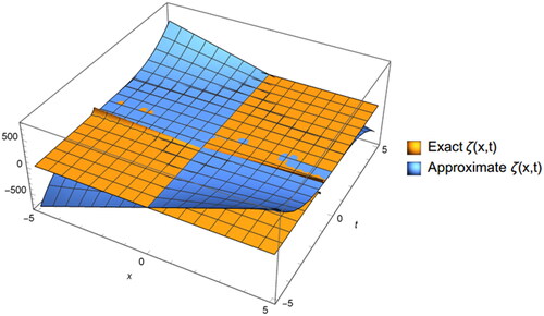
Figure 2. The 2D graph of exact and approximate solutions of Eq. (6.1)(6.1) $$\frac{\partial \zeta (x,t)}{\partial t}+\zeta \left(x,t\right)\frac{\partial \zeta \left(x,t\right)}{\partial x}-\frac{{\partial }^2\zeta \left(x,t\right)}{{\partial x}^2}=0,$$(6.1) .

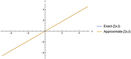
Table 1. Solution for the (first three approximations) with exact solution for example 6.1 at $t=0.1.$

$t$	$x$	Approximate solution of $\zeta \left(x,t\right)$	Exact solution of $\zeta \left(x,t\right)$
0.1	0	0	0
	0.1	0.0909	0.090909091
	0.2	0.1818	0.181818182
	0.3	0.2727	0.272727273
	0.4	0.3636	0.363636364
	0.5	0.4545	0.454545455
	0.6	0.5454	0.545454545
	0.7	0.6363	0.636363636
	0.8	0.7272	0.727272727
	0.9	0.8181	0.818181818
	1	0.909	0.909090909

Example 6.2.

Consider the homogeneous singular one-dimensional Burgers’ equation (6.3) $$\frac{\partial \zeta }{\partial t}-\frac{1}{x}\frac{\partial }{\partial x}\left(x\frac{\partial \zeta }{\partial x}\right)-2\mathrm{ }\zeta \frac{\partial \zeta }{\partial x}+\frac{\partial {\zeta }^2}{\partial x}=x^2{e}^t-4e^t,$$(6.3) subject to (6.4) $$\zeta \left(x,0\right)=x^2.$$(6.4)

By following similar above steps, we obtain (6.5) $$\begin{array}{c}\begin{array}{c}\sum _{n=0}^{\mathrm{\infty }}{\zeta }_n\left(x,t\right)=x^2+{\mathcal{G}}_r^{-1}{\mathcal{G}}_s^{-1}\left[\frac{1}{s}\left({\mathcal{G}}_x{\mathcal{G}}_t\left[x^2{e}^t-4e^t\right]\right)\right]-{\mathcal{G}}_r^{-1}{\mathcal{G}}_s^{-1}\left[\frac{r}{s}\underset{0}{\overset{r}{\int }}\frac{1}{r}\left({\mathcal{G}}_x{\mathcal{G}}_t\left[\frac{\partial }{\partial x}\left(x\left(\sum _{n=0}^{\mathrm{\infty }}{\zeta }_n\right)\right)\right]\right)\mathit{\text{dr}}\right]\\ \mathrm{ }\\ -2\mathrm{ }{\mathcal{G}}_r^{-1}{\mathcal{G}}_s^{-1}\left[\frac{r}{s}\underset{0}{\overset{r}{\int }}\frac{1}{r}\left({\mathcal{G}}_x{\mathcal{G}}_t\left[x\sum _{n=0}^{\mathrm{\infty }}{A}_n\right]\right)\mathit{\text{dr}}\right]+{\mathcal{G}}_r^{-1}{\mathcal{G}}_s^{-1}\left[\frac{r}{s}\underset{0}{\overset{r}{\int }}\frac{1}{r}\left({\mathcal{G}}_x{\mathcal{G}}_t\left[x\sum _{n=0}^{\mathrm{\infty }}{C}_n\right]\right)\mathit{\text{dr}}\right].\end{array}\\ \mathrm{ }\end{array}$$(6.5)

Using Equations (4.21)(4.21) $${\zeta }_0=k\left(x\right)+{\mathcal{G}}_r^{-1}{\mathcal{G}}_s^{-1}\left[\frac{1}{s}{\mathcal{ }\mathcal{G}}_x{\mathcal{G}}_t\left[g\left(x,t\right)\right]\right].$$(4.21) and (4.22)(4.22) $$\begin{array}{c}{\zeta }_{n+1}\left(x,t\right)=-{\mathcal{G}}_r^{-1}{\mathcal{G}}_s^{-1}\left[\frac{r}{s}\underset{0}{\overset{r}{\int }}\frac{1}{r}\left({\mathcal{G}}_x{\mathcal{G}}_t\left[\frac{\partial }{\partial x}\left(x\mathrm{ }{\zeta }_n\left(x,t\right)\right)\right]\right)\mathit{\text{dr}}\right]+\lambda \mathrm{ }{\mathcal{G}}_r^{-1}{\mathcal{G}}_s^{-1}\left[\frac{r}{s}\underset{0}{\overset{r}{\int }}\frac{1}{r}\left({\mathcal{G}}_x{\mathcal{G}}_t\left[x\mathrm{ }{A}_n\right]\right)\mathit{\text{dr}}\right]\\ \mathrm{ }\\ +\alpha \mathrm{ }{G}_r^{-1}{G}_s^{-1}\left[\frac{r}{s}\underset{0}{\overset{r}{\int }}\frac{1}{r}\left({\mathcal{G}}_x{\mathcal{G}}_t\left[x\mathrm{ }{B}_n\right]\right)\mathit{\text{dr}}\right].\end{array}$$(4.22) the components are given by $${\zeta }_0=x^2+{\mathcal{G}}_r^{-1}{\mathcal{G}}_s^{-1}\left[\frac{1}{s}{\mathcal{ }\mathcal{G}}_x{\mathcal{G}}_t\left(x^2{e}^t-4e^t\right)\right]=x^2+{\mathcal{G}}_r^{-1}{\mathcal{G}}_s^{-1}\left[\frac{1}{s}\left(\frac{2}{r^2}\left(\frac{s}{s-1}\right)-\frac{4s}{s-1}\right)\right]$$ $$=x^2+{\mathcal{G}}_r^{-1}{\mathcal{G}}_s^{-1}\left[\frac{1}{s}\left(\frac{2}{r^2}\left(\frac{s^2}{s-1}-s\right)+4s\left(1-\frac{s}{s-1}\right)\right)\right]$$ $$=x^2+{\mathcal{G}}_r^{-1}{\mathcal{G}}_s^{-1}\left[\frac{1}{s}\left(\frac{2}{r^2}\left(\frac{s^2}{s-1}\right)-\frac{4s^2}{s-1}-\frac{2s}{r^2}+4s\right)\right]$$ $$=x^2+{\mathcal{G}}_r^{-1}{\mathcal{G}}_s^{-1}\left[\left(\frac{2}{r^2}\left(\frac{s}{s-1}\right)-\frac{4s}{s-1}-\frac{2}{r^2}+4\right)\right]=x^2+x^2{e}^t-4e^t-x^2+4=x^2{e}^t-4e^t+4.$$ $${\zeta }_1=-{\mathcal{G}}_r^{-1}{\mathcal{G}}_s^{-1}\left[\frac{r}{s}\underset{0}{\overset{r}{\int }}\frac{1}{r}\left({\mathcal{G}}_x{\mathcal{G}}_t\left[\frac{\partial }{\partial x}\left(x\frac{\partial {\zeta }_0}{\partial x}\right)+2x{\zeta }_0\frac{\partial {\zeta }_0}{\partial x}-x\frac{\partial {{\zeta }_0}^2}{\partial x}\right]\right)\mathit{\text{dr}}\right]$$ $$=-{\mathcal{G}}_r^{-1}{\mathcal{G}}_s^{-1}[\frac{r}{s}\underset{0}{\overset{r}{\int }}\frac{1}{r}({\mathcal{G}}_x{\mathcal{G}}_t[4{\mathit{\text{xe}}}^t+4x^2(x^2{e}^t-4e^t+4)e^t-(4x^4{e}^{2t}-16x^2{e}^{2t}+16x^2{e}^t)])\mathit{\text{dr}}]$$ $$=-{\mathcal{G}}_r^{-1}{\mathcal{G}}_s^{-1}\left[\frac{r}{s}\underset{0}{\overset{r}{\int }}\frac{1}{r}\left({\mathcal{G}}_x{\mathcal{G}}_t\left[\left(4{\mathit{\text{xe}}}^t\right)\right]\right)\mathit{\text{dr}}\right]={\mathcal{G}}_r^{-1}{\mathcal{G}}_s^{-1}\left[\frac{4r}{s}\underset{0}{\overset{r}{\int }}\frac{d}{\mathit{\text{dr}}}\left(\frac{1}{r}\left(\frac{s}{s-1}\right)\right)\mathit{\text{dr}}\right]=4e^t-4.$$

In a similar way, we obtain $${\zeta }_2={\zeta }_3={\zeta }_4=\dots =0.$$

Thus, it is obvious that the self-canceling some terms appear among various components and following terms, then we have $$\zeta \left(x,t\right)={\zeta }_0+{\zeta }_1.$$

Therefore, the exact solution is given by $$\zeta \left(x,t\right)=x^2{e}^t.$$

The following figures, Figures 3 and 4 illustrates the 3D and 2D graph of exact and approximate solutions of Example 6.2 (Table 2).

Figure 3. The 3D graph of exact and approximate solutions of Eq. (6.3)(6.3) $$\frac{\partial \zeta }{\partial t}-\frac{1}{x}\frac{\partial }{\partial x}\left(x\frac{\partial \zeta }{\partial x}\right)-2\mathrm{ }\zeta \frac{\partial \zeta }{\partial x}+\frac{\partial {\zeta }^2}{\partial x}=x^2{e}^t-4e^t,$$(6.3) .

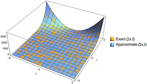
Figure 4. The 2D graph of exact and approximate solution of Eq. (6.3)(6.3) $$\frac{\partial \zeta }{\partial t}-\frac{1}{x}\frac{\partial }{\partial x}\left(x\frac{\partial \zeta }{\partial x}\right)-2\mathrm{ }\zeta \frac{\partial \zeta }{\partial x}+\frac{\partial {\zeta }^2}{\partial x}=x^2{e}^t-4e^t,$$(6.3) .

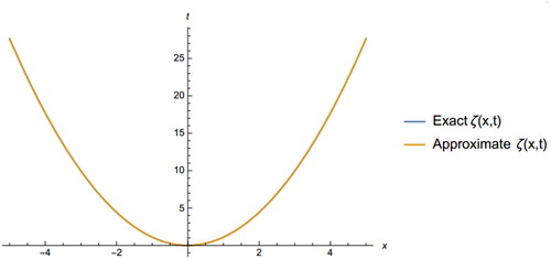
Table 2. Solution for the (first three approximations) with exact solution for example 6.2 at $t=0.1.$

$t$	$x$	Approximate solution of $\zeta \left(x,t\right)$	Exact solution of $\zeta \left(x,t\right)$
0.1	0	0	0
	0.1	0.011051709	0.011051709
	0.2	0.044206837	0.044206837
	0.3	0.099465383	0.099465383
	0.4	0.176827347	0.176827347
	0.5	0.27629273	0.27629273
	0.6	0.397861531	0.397861531
	0.7	0.54153375	0.54153375
	0.8	0.707309388	0.707309388
	0.9	0.895188444	0.895188444
	1	1.105170918	1.105170918

Example 6.3.

Consider the homogeneous regular one-dimensional coupled Burgers’ equation (6.6) $$\begin{array}{c}\frac{\partial \zeta (x,t)}{\partial t}-\frac{{\partial }^2\zeta (x,t)}{{\partial x}^2}-2\mathrm{ }\zeta \left(x,t\right)\frac{\partial \zeta \left(x,t\right)}{\partial x}+\frac{\partial }{\partial x}\left(\zeta \left(x,t\right)\xi \left(x,t\right)\right)=0,\\ \frac{\partial \xi (x,t)}{\partial t}-\frac{{\partial }^2\xi \left(x,t\right)}{{\partial x}^2}-2\mathrm{ }\xi \left(x,t\right)\frac{\partial \xi \left(x,t\right)}{\partial x}+\frac{\partial }{\partial x}\left(\zeta \left(x,t\right)\xi (x,t\right)=0,\end{array}$$(6.6) subject to (6.7) $$\zeta \left(x,0\right)=\mathrm{\text{sin}}\hspace{0.17em}x,\xi \left(x,0\right)=\mathrm{\text{sin}}\hspace{0.17em}x.$$(6.7)

Using Equations (5.10)(5.10) $$\begin{array}{c}{\zeta }_0=u_1\left(x\right)+{\mathcal{G}}_r^{-1}{\mathcal{G}}_s^{-1}\left[\frac{1}{s}{\mathcal{ }\mathcal{G}}_x{\mathcal{G}}_t\left[u\left(x,t\right)\right]\right],\\ {\xi }_0=v_1\left(x\right)+{\mathcal{G}}_r^{-1}{\mathcal{G}}_s^{-1}\left[\frac{1}{s}{\mathcal{ }\mathcal{G}}_x{\mathcal{G}}_t\left[v\left(x,t\right)\right]\right].\end{array}$$(5.10) —(5.12)(5.12) $${\xi }_{n+1}={\mathcal{G}}_r^{-1}{\mathcal{G}}_s^{-1}\left[\frac{1}{s}{\mathcal{ }\mathcal{G}}_x{\mathcal{G}}_t\left[{{\xi }_n}_{\mathit{\text{xx}}}\left(x,t\right)\right]\right]-\lambda \mathrm{ }{G}_r^{-1}{\mathcal{G}}_s^{-1}\left[\frac{1}{s}{\mathcal{ }\mathcal{G}}_x{\mathcal{G}}_t\left[{\mathrm{ }B}_n\right]\right]-\beta \mathrm{ }{\mathcal{G}}_r^{-1}{\mathcal{G}}_s^{-1}\left[\frac{1}{s}{\mathcal{ }\mathcal{G}}_{\mathrm{x}}{\mathcal{G}}_t\left[C_n\right]\right].$$(5.12) , we have $$\begin{array}{c}{\zeta }_0=u_1\left(x\right)+{\mathcal{G}}_r^{-1}{\mathcal{G}}_s^{-1}\left[\frac{1}{s}{\mathcal{ }\mathcal{G}}_x{\mathcal{G}}_t\left[u\left(x,t\right)\right]\right]=\mathrm{\text{sin}}\hspace{0.17em}x,\\ {\xi }_0=v_1\left(x\right)+{\mathcal{G}}_r^{-1}{\mathcal{G}}_s^{-1}\left[\frac{1}{s}{\mathcal{ }\mathcal{G}}_x{\mathcal{G}}_t\left[v\left(x,t\right)\right]\right]=\mathrm{\text{sin}}\hspace{0.17em}x.\end{array}$$ $$\begin{array}{c}\begin{array}{c}\mathrm{ }\\ {\zeta }_1={\mathcal{G}}_r^{-1}{\mathcal{G}}_s^{-1}\left[\frac{1}{s}{\mathcal{ }\mathcal{G}}_x{\mathcal{G}}_t\left[\frac{{\partial }^2{\zeta }_0}{{\partial x}^2}+2{\zeta }_0\frac{\partial {\zeta }_0}{\partial x}-\frac{\partial }{\partial x}\left({\zeta }_0{\xi }_0\right)\right]\right]\\ ={\mathcal{G}}_r^{-1}{\mathcal{G}}_s^{-1}\left[\frac{1}{s}{\mathcal{ }\mathcal{G}}_x{\mathcal{G}}_t\left[-\mathrm{\text{sin}}x\right]\right]={\mathcal{G}}_r^{-1}{\mathcal{G}}_s^{-1}\left[\frac{-r}{s\left(r^2+1\right)}\right]=-t\mathrm{\text{sin}}\hspace{0.17em}x.\end{array}\\ {\xi }_1={\mathcal{G}}_r^{-1}{\mathcal{G}}_s^{-1}\left[\frac{1}{s}{\mathcal{ }\mathcal{G}}_x{\mathcal{G}}_t\left[\frac{{\partial }^2{\xi }_0}{{\partial x}^2}+2{\xi }_0\frac{\partial {\xi }_0}{\partial x}-\frac{\partial }{\partial x}\left({\zeta }_0{\xi }_0\right)\right]\right]\\ ={\mathcal{G}}_r^{-1}{\mathcal{G}}_s^{-1}\left[\frac{1}{s}{\mathcal{ }\mathcal{G}}_x{\mathcal{G}}_t\left[-\mathrm{\text{sin}}\hspace{0.17em}x\right]\right]={\mathcal{G}}_r^{-1}{\mathcal{G}}_s^{-1}\left[\frac{-r}{s\left(r^2+1\right)}\right]=-t\mathrm{\text{sin}}\hspace{0.17em}x\mathrm{ }.\end{array}$$ $$\begin{array}{c}{\zeta }_2={\mathcal{G}}_r^{-1}{\mathcal{G}}_s^{-1}[\frac{1}{s}{\mathcal{ }\mathcal{G}}_x{\mathcal{G}}_t[\frac{{\partial }^2{\zeta }_1}{{\partial x}^2}+2({\zeta }_0\frac{\partial {\zeta }_1}{\partial x}+{\zeta }_1\frac{\partial {\zeta }_0}{\partial x})-\frac{\partial }{\partial x}({\zeta }_0{\xi }_1+{\zeta }_1{\xi }_0)]]\\ ={\mathcal{G}}_r^{-1}{\mathcal{G}}_s^{-1}\left[\frac{1}{s}{\mathcal{ }\mathcal{G}}_x{\mathcal{G}}_t\left[t\mathrm{\text{sin}}\hspace{0.17em}x\right]\right]={\mathcal{G}}_r^{-1}{\mathcal{G}}_s^{-1}\left[\frac{r}{s^2\left(r^2+1\right)}\right]=\frac{t^2}{2}\mathrm{\text{sin}}\hspace{0.17em}x.\end{array}$$ $$\begin{array}{c}{\xi }_2={\mathcal{G}}_r^{-1}{\mathcal{G}}_s^{-1}[\frac{1}{s}{\mathcal{ }\mathcal{G}}_x{\mathcal{G}}_t[\frac{{\partial }^2{\xi }_1}{{\partial x}^2}+2({\xi }_0\frac{\partial {\xi }_1}{\partial x}+{\xi }_1\frac{\partial {\xi }_0}{\partial x})-\frac{\partial }{\partial x}({\zeta }_0{\xi }_1+{\zeta }_1{\xi }_0)]]\\ ={\mathcal{G}}_r^{-1}{\mathcal{G}}_s^{-1}\left[\frac{1}{s}{\mathcal{ }\mathcal{G}}_x{\mathcal{G}}_t\left[t\mathrm{\text{sin}}\hspace{0.17em}x\right]\right]={\mathcal{G}}_r^{-1}{\mathcal{G}}_s^{-1}\left[\frac{r}{s^2\left(r^2+1\right)}\right]=\frac{t^2}{2}\mathrm{\text{sin}}\hspace{0.17em}x.\end{array}$$

And $${\zeta }_3={\mathcal{G}}_r^{-1}{\mathcal{G}}_s^{-1}[\frac{1}{s}{\mathcal{ }\mathcal{G}}_x{\mathcal{G}}_t[\frac{{\partial }^2{\zeta }_2}{{\partial x}^2}+2({\zeta }_0\frac{\partial {\zeta }_2}{\partial x}+{\zeta }_1\frac{\partial {\zeta }_1}{\partial x}+{\zeta }_2\frac{\partial {\zeta }_0}{\partial x})-\frac{\partial }{\partial x}({\zeta }_0{\xi }_2+{\zeta }_1{\xi }_1+{\zeta }_2{\xi }_0)]]=-\frac{t^3}{6}\mathrm{\text{sin}}\hspace{0.17em}x,$$ $${\xi }_3={\mathcal{G}}_r^{-1}{\mathcal{G}}_s^{-1}[\frac{1}{s}{\mathcal{ }\mathcal{G}}_x{\mathcal{G}}_t[\frac{{\partial }^2{\xi }_2}{{\partial x}^2}+2({\xi }_0\frac{\partial {\xi }_2}{\partial x}+{\xi }_1\frac{\partial {\xi }_1}{\partial x}+{\xi }_2\frac{\partial {\xi }_0}{\partial x})-\frac{\partial }{\partial x}({\zeta }_0{\xi }_2+{\zeta }_1{\xi }_1+{\zeta }_2{\xi }_0)]]=-\frac{t^3}{6}\mathrm{\text{sin}}\hspace{0.17em}x.$$ and similar to the other components. Therefore, by using Equation (5.6)(5.6) $$\zeta \left(x,t\right)=\sum _{n=0}^{\mathrm{\infty }}{\zeta }_n\left(x,t\right),\xi \left(x,t\right)=\sum _{n=0}^{\mathrm{\infty }}{\xi }_n\left(x,t\right).$$(5.6) , the series solutions are given by $$\begin{array}{c}\zeta (x,t)={\zeta }_0+{\zeta }_1+{\zeta }_2+...=(1-t+\frac{t^2}{2!}-\frac{t^3}{3!}+...)\text{sin}\hspace{0.17em}x,\\ \xi (x,t)={\xi }_0+{\xi }_1+{\xi }_2+...=(1-t+\frac{t^2}{2!}-\frac{t^3}{3!}+...)\text{sin}\hspace{0.17em}x.\end{array}$$ and hence the exact solutions is $$\zeta \left(x,t\right)=e^{-t}\mathrm{\text{sin}}\hspace{0.17em}x,\hspace{0.5em}\xi \left(x,t\right)=e^{-t}\mathrm{\text{sin}}\hspace{0.17em}x.$$

The following figures, Figures 5 and 6 illustrates the 3D and 2D graph of exact and approximate solutions of Example 6.3 (Table 3).

Figure 5. The 3D graph of exact and approximate solutions of Eq. (6.6)(6.6) $$\begin{array}{c}\frac{\partial \zeta (x,t)}{\partial t}-\frac{{\partial }^2\zeta (x,t)}{{\partial x}^2}-2\mathrm{ }\zeta \left(x,t\right)\frac{\partial \zeta \left(x,t\right)}{\partial x}+\frac{\partial }{\partial x}\left(\zeta \left(x,t\right)\xi \left(x,t\right)\right)=0,\\ \frac{\partial \xi (x,t)}{\partial t}-\frac{{\partial }^2\xi \left(x,t\right)}{{\partial x}^2}-2\mathrm{ }\xi \left(x,t\right)\frac{\partial \xi \left(x,t\right)}{\partial x}+\frac{\partial }{\partial x}\left(\zeta \left(x,t\right)\xi (x,t\right)=0,\end{array}$$(6.6) .

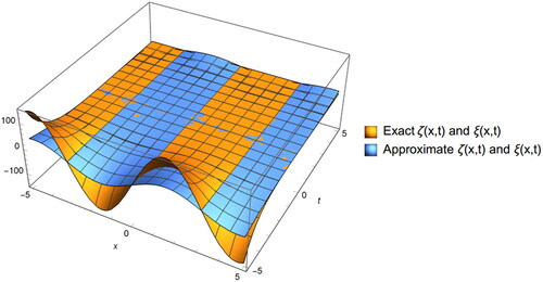
Figure 6. The 2D graph of exact solution of Eq. (6.6)(6.6) $$\begin{array}{c}\frac{\partial \zeta (x,t)}{\partial t}-\frac{{\partial }^2\zeta (x,t)}{{\partial x}^2}-2\mathrm{ }\zeta \left(x,t\right)\frac{\partial \zeta \left(x,t\right)}{\partial x}+\frac{\partial }{\partial x}\left(\zeta \left(x,t\right)\xi \left(x,t\right)\right)=0,\\ \frac{\partial \xi (x,t)}{\partial t}-\frac{{\partial }^2\xi \left(x,t\right)}{{\partial x}^2}-2\mathrm{ }\xi \left(x,t\right)\frac{\partial \xi \left(x,t\right)}{\partial x}+\frac{\partial }{\partial x}\left(\zeta \left(x,t\right)\xi (x,t\right)=0,\end{array}$$(6.6) .

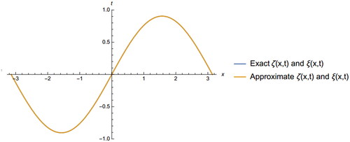
Table 3. Solution for the (first three approximations) with exact solution for example 6.3 at $t=0.1.$

$t$	$x$	Approximate solution of $\zeta \left(x,t\right)$ and $\xi (x,t)$	Exact solution of $\zeta \left(x,t\right)$ and $\xi (x,t)$
0.1	0	0	0
	$\pi /6$	0.4524166666666667	0.45241870901797976
	$\pi /3$	0.7836086528576196	0.7836121903138608
	$\pi /2$	0.9048333333333334	0.9048374180359595
	$2\pi /3$	0.7836086528576196	0.7836121903138608
	$5\pi /6$	0.4524166666666667	0.45241870901797976
	$\pi$	0	0

Example 6.4.

Consider the homogeneous singular one-dimensional coupled Burgers’ equation (6.8) $$\begin{array}{c}\frac{\partial \zeta }{\partial t}-\frac{1}{x}\frac{\partial }{\partial x}\left(x\frac{\partial \zeta }{\partial x}\right)-2\mathrm{ }\zeta \frac{\partial \zeta }{\partial x}+\frac{\partial }{\partial x}\left(\mathrm{\zeta \xi }\right)=x^2{e}^t-4e^t,\\ \frac{\partial \xi }{\partial t}-\frac{1}{x}\frac{\partial }{\partial x}\left(x\frac{\partial \xi }{\partial x}\right)-2\mathrm{ }\xi \frac{\partial \xi }{\partial x}+\frac{\partial }{\partial x}\left(\mathrm{\zeta \xi }\right)=x^2{e}^t-4e^t,\end{array}$$(6.8) subject to (6.9) $$\zeta \left(x,0\right)=x^2,\xi \left(x,0\right)=x^2.$$(6.9)

By following similar above steps, we obtain (6.10) $$\begin{array}{c}\begin{array}{c}\sum _{n=0}^{\mathrm{\infty }}{\zeta }_n\left(x,t\right)=x^2+{\mathcal{G}}_r^{-1}{\mathcal{G}}_s^{-1}\left[\frac{1}{s}\left({\mathcal{ }\mathcal{G}}_x{\mathcal{G}}_t\left[x^2{e}^t-4e^t\right]\right)\right]-\mathrm{ }{\mathcal{G}}_r^{-1}{\mathcal{G}}_s^{-1}\left[\frac{r}{s}\underset{0}{\overset{r}{\int }}\frac{1}{r}\left({\mathcal{G}}_x{\mathcal{G}}_t\left[\frac{\partial }{\partial x}\left(x\left(\sum _{n=0}^{\mathrm{\infty }}{\zeta }_n\right)\right)\right]\right)\mathit{\text{dr}}\right]\\ \mathrm{ }\\ -2\mathrm{ }{\mathcal{G}}_r^{-1}{\mathcal{G}}_s^{-1}\left[\frac{r}{s}\underset{0}{\overset{r}{\int }}\frac{1}{r}\left({\mathcal{G}}_x{\mathcal{G}}_t\left[x\sum _{n=0}^{\mathrm{\infty }}{A}_n\right]\right)\mathit{\text{dr}}\right]+{\mathcal{G}}_r^{-1}{\mathcal{G}}_s^{-1}\left[\frac{r}{s}\underset{0}{\overset{r}{\int }}\frac{1}{r}\left({\mathcal{G}}_x{\mathcal{G}}_t\left[x\sum _{n=0}^{\mathrm{\infty }}{C}_n\right]\right)\mathit{\text{dr}}\right].\end{array}\\ \mathrm{ }\end{array}$$(6.10)

And (6.11) $$\begin{array}{c}\begin{array}{c}\sum _{n=0}^{\mathrm{\infty }}{\xi }_n\left(x,t\right)=x^2+{\mathcal{G}}_r^{-1}{\mathcal{G}}_s^{-1}\left[\frac{1}{s}\left({\mathcal{ }\mathcal{G}}_x{\mathcal{G}}_t\left[x^2{e}^t-4e^t\right]\right)\right]-\mathrm{ }{\mathcal{G}}_r^{-1}{\mathcal{G}}_s^{-1}\left[\frac{r}{s}\underset{0}{\overset{r}{\int }}\frac{1}{r}\left({\mathcal{G}}_x{\mathcal{G}}_t\left[\frac{\partial }{\partial x}\left(x\left(\sum _{n=0}^{\mathrm{\infty }}{v}_n\right)\right)\right]\right)\mathit{\text{dr}}\right]\\ \mathrm{ }\\ -2\mathrm{ }{\mathcal{G}}_r^{-1}{\mathcal{G}}_s^{-1}\left[\frac{r}{s}\underset{0}{\overset{r}{\int }}\frac{1}{r}\left({\mathcal{G}}_x{\mathcal{G}}_t\left[x\sum _{n=0}^{\mathrm{\infty }}{B}_n\right]\right)\mathit{\text{dr}}\right]+{\mathcal{G}}_r^{-1}{\mathcal{G}}_s^{-1}\left[\frac{r}{s}\underset{0}{\overset{r}{\int }}\frac{1}{r}\left({\mathcal{G}}_x{\mathcal{G}}_t\left[x\sum _{n=0}^{\mathrm{\infty }}{C}_n\right]\right)\mathit{\text{dr}}\right].\end{array}\\ \mathrm{ }\end{array}$$(6.11)

Using Equations (5.25)(5.25) $$\begin{array}{c}{\zeta }_0=u_1\left(x\right)+{\mathcal{G}}_r^{-1}{\mathcal{G}}_s^{-1}\left[\frac{1}{\mathrm{s}}{\mathcal{ }\mathcal{G}}_x{\mathcal{G}}_t\left[u\left(x,t\right)\right]\right],\\ {\xi }_0=v_1\left(x\right)+{\mathcal{G}}_r^{-1}{\mathcal{G}}_s^{-1}\left[\frac{1}{s}{\mathcal{ }\mathcal{G}}_x{\mathcal{G}}_t\left[v\left(x,t\right)\right]\right],\end{array}$$(5.25) —(5.27)(5.27) $$\begin{array}{c}{\xi }_{n+1}\left(x,t\right)={-\mathcal{G}}_r^{-1}{\mathcal{G}}_s^{-1}\left[\frac{r}{s}\underset{0}{\overset{r}{\int }}\frac{1}{r}\left({\mathcal{G}}_x{\mathcal{G}}_t\left[\frac{\partial }{\partial x}\left(x\mathrm{ }{\xi }_n\left(x,t\right)\right)\right]\right)\mathit{\text{dr}}\right]+\lambda \mathrm{ }{\mathcal{G}}_r^{-1}{\mathcal{G}}_s^{-1}\left[\frac{r}{s}\underset{0}{\overset{r}{\int }}\frac{1}{r}\left({\mathcal{G}}_x{\mathcal{G}}_t\left[x\mathrm{ }{B}_n\right]\right)\mathit{\text{dr}}\right]\\ +\beta \mathrm{ }{G}_r^{-1}{G}_s^{-1}\left[\frac{r}{s}\underset{0}{\overset{r}{\int }}\frac{1}{r}\left({\mathcal{G}}_x{\mathcal{G}}_t\left[x\mathrm{ }{C}_n\right]\right)\mathit{\text{dr}}\right],\\ \mathrm{ }\end{array}$$(5.27) the components are given by $${\zeta }_0=x^2+{\mathcal{G}}_r^{-1}{\mathcal{G}}_s^{-1}\left[\frac{1}{s}{\mathcal{ }\mathcal{G}}_x{\mathcal{G}}_t\left(x^2{e}^t-4e^t\right)\right]=x^2+{\mathcal{G}}_r^{-1}{\mathcal{G}}_s^{-1}\left[\frac{1}{s}\left(\frac{2}{r^2}\left(\frac{s}{s-1}\right)-\frac{4s}{s-1}\right)\right]$$ $$=x^2+{\mathcal{G}}_r^{-1}{\mathcal{G}}_s^{-1}\left[\frac{1}{s}\left(\frac{2}{r^2}\left(\frac{s^2}{s-1}-s\right)+4s\left(1-\frac{s}{s-1}\right)\right)\right]$$ $$=x^2+{\mathcal{G}}_r^{-1}{\mathcal{G}}_s^{-1}\left[\frac{1}{s}\left(\frac{2}{r^2}\left(\frac{s^2}{s-1}\right)-\frac{4s^2}{s-1}-\frac{2s}{r^2}+4s\right)\right]$$ $$=x^2+{\mathcal{G}}_r^{-1}{\mathcal{G}}_s^{-1}\left[\left(\frac{2}{r^2}\left(\frac{s}{s-1}\right)-\frac{4s}{s-1}-\frac{2}{r^2}+4\right)\right]$$ $$=x^2+x^2{e}^t-4e^t-x^2+4=x^2{e}^t-4e^t+4.$$

In a similar way, we obtain $${\xi }_0=x^2{e}^t-4e^t+4.$$ $${\zeta }_1=-\mathrm{ }{\mathcal{G}}_r^{-1}{\mathcal{G}}_s^{-1}[\frac{r}{s}\underset{0}{\overset{r}{\int }}\frac{1}{r}({\mathcal{G}}_x{\mathcal{G}}_t[\frac{\partial }{\partial x}(x\frac{\partial {\zeta }_0}{\partial x})+2x{\zeta }_0\frac{\partial {\zeta }_0}{\partial x}-x\frac{\partial }{\partial x}({\zeta }_0{\xi }_0)])\mathit{\text{dr}}]$$ $$=-{\mathcal{G}}_r^{-1}{\mathcal{G}}_s^{-1}[\frac{r}{s}\underset{0}{\overset{r}{\int }}\frac{1}{r}({\mathcal{G}}_x{\mathcal{G}}_t[4{\mathit{\text{xe}}}^t+4x^2(x^2{e}^t-4e^t+4)e^t-(4x^4{e}^{2t}-16x^2{e}^{2t}+16x^2{e}^t)])\mathit{\text{dr}}]$$ $$=-\mathrm{ }{\mathcal{G}}_r^{-1}{\mathcal{G}}_s^{-1}\left[\frac{r}{s}\underset{0}{\overset{r}{\int }}\frac{1}{r}\left({\mathcal{ }\mathcal{G}}_x{\mathcal{G}}_t\left[\left(4{\mathit{\text{xe}}}^t\right)\right]\right)\mathit{\text{dr}}\right]={\mathcal{G}}_r^{-1}{\mathcal{G}}_s^{-1}\left[\frac{4r}{s}\underset{0}{\overset{r}{\int }}\frac{d}{\mathit{\text{dr}}}\left(\frac{1}{r}\left(\frac{s}{s-1}\right)\right)\mathit{\text{dr}}\right]$$ $$={\mathcal{G}}_r^{-1}{\mathcal{G}}_s^{-1}\left[\frac{4}{s}\underset{0}{\overset{r}{\int }}\left(\frac{s}{s-1}\right)\mathit{\text{dr}}\right]={\mathcal{G}}_r^{-1}{\mathcal{G}}_s^{-1}\left[\frac{4}{s}\left(\frac{s^2}{s-1}-s\right)\right]=4e^t-4.$$

In a similar way, we obtain $${\xi }_1=4e^t-4.$$ $${\zeta }_2={\zeta }_3={\zeta }_4=\dots =0.$$ $${\xi }_2={\xi }_3={\xi }_4=\dots =0.$$

Thus it is obvious that the self-canceling some terms appear among various components and following terms, then we have $$\zeta \left(x,t\right)={\zeta }_0+{\zeta }_1,\xi \left(x,t\right)={\xi }_0+{\xi }_1\bullet$$

Therefore, the exact solution is given by $$\zeta \left(x,t\right)=x^2{e}^t,\xi \left(x,t\right)=x^2{e}^t.$$

The following figures, Figures 7 and 8 illustrates the 3D and 2D graph of exact and approximate solutions of Example 6.4 (Table 4).

Figure 7. The 3D graph of exact and approximate solutions of Eq. (6.8)(6.8) $$\begin{array}{c}\frac{\partial \zeta }{\partial t}-\frac{1}{x}\frac{\partial }{\partial x}\left(x\frac{\partial \zeta }{\partial x}\right)-2\mathrm{ }\zeta \frac{\partial \zeta }{\partial x}+\frac{\partial }{\partial x}\left(\mathrm{\zeta \xi }\right)=x^2{e}^t-4e^t,\\ \frac{\partial \xi }{\partial t}-\frac{1}{x}\frac{\partial }{\partial x}\left(x\frac{\partial \xi }{\partial x}\right)-2\mathrm{ }\xi \frac{\partial \xi }{\partial x}+\frac{\partial }{\partial x}\left(\mathrm{\zeta \xi }\right)=x^2{e}^t-4e^t,\end{array}$$(6.8) .

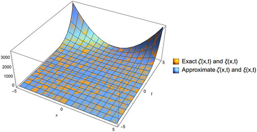
Figure 8. The 2D graph of exact and approximate solution of Eq. (6.8)(6.8) $$\begin{array}{c}\frac{\partial \zeta }{\partial t}-\frac{1}{x}\frac{\partial }{\partial x}\left(x\frac{\partial \zeta }{\partial x}\right)-2\mathrm{ }\zeta \frac{\partial \zeta }{\partial x}+\frac{\partial }{\partial x}\left(\mathrm{\zeta \xi }\right)=x^2{e}^t-4e^t,\\ \frac{\partial \xi }{\partial t}-\frac{1}{x}\frac{\partial }{\partial x}\left(x\frac{\partial \xi }{\partial x}\right)-2\mathrm{ }\xi \frac{\partial \xi }{\partial x}+\frac{\partial }{\partial x}\left(\mathrm{\zeta \xi }\right)=x^2{e}^t-4e^t,\end{array}$$(6.8) .

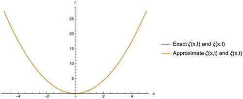
Table 4. Solution for the (first three approximations) with exact solution for example 6.4 at $t=0.1.$

$t$	$x$	Approximate solution of $\zeta \left(x,t\right)$ and $\xi (x,t)$	Exact solution of $\zeta \left(x,t\right)$ and $\xi (x,t)$
0.1	0	0	0
	0.1	0.011051709	0.011051709
	0.2	0.044206837	0.044206837
	0.3	0.099465383	0.099465383
	0.4	0.176827347	0.176827347
	0.5	0.27629273	0.27629273
	0.6	0.397861531	0.397861531
	0.7	0.54153375	0.54153375
	0.8	0.707309388	0.707309388
	0.9	0.895188444	0.895188444
	1	1.105170918	1.105170918

7. Discussions of results

In this section, we discuss the results obtained, as illustrated by the figures and solution tables provided. It is evident that the solutions derived using the new method closely approximate the exact solutions, with a very small error rate. In some instances, the results were nearly identical, as demonstrated in the three examples selected. This precision is one of the most significant advantages of this method.

8. Conclusions

In this study, we have explored certain properties and conditions necessary for applying the double ARA transform. We employed the double ARA decomposition method a fusion of the double ARA and Adomian decomposition method to solve the one-dimensional regular and singular coupled Burgers’ equations. We presented three problems to validate the efficacy of this novel method. Furthermore, it is important to note that this double transform, when combined with iterative numerical methods, can also be used to address nonlinear problems and equations with non-constant coefficients, as direct solutions to nonlinear issues are not feasible with transforms alone unless paired with iterative techniques. Initial conditions must also be set to zero.

Looking ahead, I plan to apply this technique to investigate fractional differential equations and nonlinear time-fractional differential equations. Specifically, I aim to utilize this method for the Burgers’ equation with fractional derivatives, anticipating lower computational demands and higher accuracy. Future research will also explore the application of the Burgers’ fractional-order equation, given its extensive applications in physics and fluid dynamics. Additionally, I will examine the presence of concrete physical phenomena and validate any practical applications in real-world scenarios.

Acknowledgements

I would like to acknowledge my colleagues Holy Quran and Islamic Sciences University for their technical advice. The author expresses his gratitude to the editor and dear unknown reviewers and for their helpful suggestions, which improved the final version of this manuscript. The author extends his sincere thanks to Dr.Nauman Ali and Dr.Ahmed Elhassan for improving the language of the manuscript. He also thanks Professor Tariq Al-Zaki and Dr. Rania Saadeh for their general review of the manuscript. I also thank Dr. Jamal Derbali and Dr. Muhammad Zain for helping me with the physics aspect, drawing solutions, and preparing their tables. Finally, I do not forget to thank my student, Muneerah Al-Ghamdi, who provided me with moral and material support.

Disclosure statement

No potential conflict of interest was reported by the author.

Appendix

Table A1. Here we present a list of the previous results double ARA transform of some special function and general properties.

$\zeta \left(x,t\right)$	${\mathcal{ }\mathcal{G}}_x{\mathcal{G}}_t\left[\zeta \left(x,t\right)\right]=\mathrm{\Phi }\left(r,s\right)$
$1$	$1$
$x^n{t}^m$	$\frac{n!m!}{r^n{s}^m}.$
$e^{\lambda \mathrm{ x}+\beta \mathrm{ t}}$	$\frac{\mathit{\text{rs}}}{(r-\lambda )(s-\beta )}.$
$\mathrm{\text{sin}}\hspace{0.17em}\mathrm{\lambda x}\mathrm{\text{sin}}\hspace{0.17em}\mathrm{\beta t}$	$\frac{\mathit{\text{λβrs}}}{\left(r^2+{\lambda }^2\right)\left(s^2+{\beta }^2\right)}.$
$\mathrm{x\zeta }\left(x,t\right)$	$-r\frac{\partial }{\partial r}\left(\frac{1}{r}\mathrm{\Phi }\left(r,s\right)\right).$
$\mathrm{t\zeta }\left(x,t\right)$	$-s\frac{\partial }{\partial s}\left(\frac{1}{s}\mathrm{\Phi }\left(r,s\right)\right).$
$x^2\zeta \left(x,t\right)$	$\frac{{\partial }^2\mathrm{\Phi }\left(r,s\right)}{\partial r^2}‐\mathrm{ }\frac{2}{r}\frac{\partial \mathrm{\Phi }\left(r,s\right)}{\partial r}+\frac{2}{r^2}\mathrm{\Phi }\left(r,s\right).$
$t^2\zeta \left(x,t\right)$	$\frac{{\partial }^2\mathrm{\Phi }\left(r,s\right)}{\partial s^2}‐\mathrm{ }\frac{2}{s}\frac{\partial \mathrm{\Phi }\left(r,s\right)}{\partial s}+\frac{2}{s^2}\mathrm{\Phi }\left(r,s\right).$
$\mathit{\text{xt}}\mathrm{ \zeta }\left(x,t\right)$	$\frac{{\partial }^2\mathrm{\Phi }\left(r,s\right)}{\partial r\partial s}-\frac{1}{s}\frac{\partial \mathrm{\Phi }\left(r,s\right)}{\partial r}-\frac{1}{r}\frac{\partial \mathrm{\Phi }\left(r,s\right)}{\partial s}+\frac{1}{\mathit{\text{rs}}}\mathrm{\Phi }\left(r,s\right).$
$\frac{\partial }{\partial x}\zeta \left(x,t\right)$	$r\mathrm{ }\mathrm{\Phi }\left(r,s\right)-r\mathrm{ }{\mathcal{G}}_t\left[\zeta \left(0,t\right)\right].$
$\frac{\partial }{\partial t}\zeta \left(x,t\right)$	$s\mathrm{ }\mathrm{\Phi }\left(r,s\right)-s\mathrm{ }{\mathcal{ }\mathcal{G}}_x\left[\zeta \left(x,0\right)\right].$
$\frac{{\partial }^2}{\partial x^2}\zeta \left(x,t\right)$	$r^2\mathrm{\Phi }\left(r,s\right)-r^{2\mathrm{ }}{\mathcal{G}}_t\left[\zeta \left(0,t\right)\right]-r\mathrm{ }{\mathcal{G}}_t\left[\frac{\partial }{\partial x}\zeta \left(0,t\right)\right].$
$\frac{{\partial }^2}{\partial t^2}\zeta \left(x,t\right)$	$s^2\mathrm{\Phi }\left(r,s\right)-s^2{\mathcal{ }\mathcal{G}}_x\left[\zeta \left(x,0\right)\right]-s\mathrm{ }{\mathcal{ }\mathcal{G}}_x\left[\frac{\partial }{\partial t}\zeta \left(x,0\right)\right].$
$x\frac{\partial }{\partial t}\zeta \left(x,t\right)$	$\mathit{\text{rs}}\frac{d}{\mathit{\text{dr}}}\left(\frac{1}{r}{\mathcal{ }\mathcal{G}}_x\left[\zeta \left(x,0\right)\right]\right)-\mathit{\text{rs}}\frac{\partial }{\partial r}\left(\frac{1}{r}\mathrm{\Phi }\left(r,s\right)\right).$
$t\frac{\partial }{\partial x}\zeta \left(x,t\right)$	$\mathit{\text{rs}}\frac{d}{\mathit{\text{ds}}}\left(\frac{1}{s}{\mathcal{ }\mathcal{G}}_t\left[\zeta \left(0,t\right)\right]\right)-\mathit{\text{rs}}\frac{\partial }{\partial r}\left(\frac{1}{s}\mathrm{\Phi }\left(r,s\right)\right).$

References

- Ahmed, S. A., Elzaki, T. M., & Hassan, A. A. (2020). Solution of integral differential equations by new double integral transform (Laplace–Sumudu transform). Abstract and Applied Analysis, 2020, 1–7. doi:10.1155/2020/4725150
- Ahmed, Z., Idrees, M. I., Belgacem, F. M., & Perveen, Z. (2019). On the convergence of double Sumudu transform. Journal of Nonlinear Sciences and Applications, 13(3), 154–162. doi:10.22436/jnsa.013.03.04
- Alam, M. N., & Tunc, C. (2016). An analytical method for solving exact solutions of the nonlinear Bogoyavlenskii equation and the nonlinear diffusive predator-prey system. Alexandria Engineering Journal, 55(2), 1855–1865. doi:10.1016/j.aej.2016.04.024
- Alam, M. N., & Tunç, C. (2020). New solitary wave structures to the (2 + 1)-dimensional KD and KP equations with spatio-temporal dispersion. Journal of King Saud University - Science, 32(8), 3400–3409. doi:10.1016/j.jksus.2020.09.027
- Alfaqeih, S., & Misirli, E. (2020). On double Shehu transform and its properties with applications. International Journal of Analysis and Applications, 18(3), 381–395. doi:10.28924/2291-8639-18-2020-381
- Al-Omari, S. K. Q. (2012). Generalized functions for double Sumudu transformation. International Journal of Algebra, 6(3), 139–146.
- Burgers, J. M. (1948). A mathematical model illustrating the theory of turbulence. Advances in Applied Mechaincs, 1, 171–199. doi:10.1016/S0065-2156(08)70100-5
- Burqan, A., Saadeh, R., & Qazza, A. (2021). A novel numerical approach in solving fractional neutral pantograph equations via the ARA integral transform. Symmetry, 14(1), 50. doi:10.3390/sym14010050
- Constanda, C. (2018). Solution techniques for elementary partial differential equations (3rd ed.). New York: Chapman and Hall/CRC. doi:10.1201/9781315381442
- Dhunde, R. R., Bhondge, N. M., & Dhongle, P. R. (2013). Some remarks on the properties of double Laplace transforms. International Journal of Applied Physics and Mathematics, 3(4), 293–295. doi:10.7763/IJAPM.2013.V3.224
- Dhunde, R., & Waghmare, G. (2017). Double Laplace transform in mathematical physics. International Journal of Theoretical and Mathematical Physics, 7(1), 14–20. doi:10.5923/j.ijtmp.20170701.04
- Eddine, N. C., & Ragusa, M. A. (2022). Generalized critical Kirchhoff-type potential systems with neumann boundary conditions. Applicable Analysis, 101(11), 3958–3988. doi:10.1080/00036811.2022.2057305
- Eltayeb, H., Bachar, I., & Kılıçman, A. (2019). On conformable double Laplace transform and one dimensional fractional coupled Burgers’ equation. Symmetry, 11(3), 417. doi:10.5923/j.ijtmp.20170701.04
- Eltayeb, H., & Kilicman, A. (2010). On double Sumudu transform and double Laplace transform. Malaysian Journal of Mathematical Sciences, 4(1), 17–30.
- Eltayeb, H., & Kiliçman, A. (2013). A note on double Laplace transform and telegraphic equations. Abstract and Applied Analysis, 2013, 1–6. doi:10.1155/2013/932578
- Eshag, M. O. (2017). On double Laplace transform and double Sumudu transform. American Journal of Engineering Research, 6(5), 312–317.
- Evans, L. (2010). Partial differential equations (Vol. 19). American Mathematical Society. doi:10.1090/gsm/019
- Hamza, A. E., & Elzaki, T. M. (2015). Application of homotopy perturbation and Sumudu transform method for solving Burgers equations. American Journal of Theoretical and Applied Statistics, 4(6), 480. doi:10.11648/j.ajtas.20150406.18
- Idrees, M. I., Ahmed, Z., Awais, M., & Perveen, Z. (2018). On the convergence of double Elzaki transform. International Journal of Advanced and Applied Sciences, 5(6), 19–24. doi:10.21833/ijaas.2018.06.003
- Islam, S., Alam, M. N., Fayz-Al-Asad, M., & Tunç, C. (2021). An analytical technique for solving new computational solutions of the modified Zakharov-Kuznetsov equation arising in electrical engineering. Journal of Applied and Computational Mechanics, 7(2), 715–726.
- Mohamed, M. Z., Hamza, A. E., & Sedeeg, A. K. H. (2023). Conformable double Sumudu transformations an efficient approximation solutions to the fractional coupled Burger’s equation. Ain Shams Engineering Journal, 14(3) doi:10.1016/j.asej.2022.101879
- Nee, J., & Duan, J. (1998). Limit set of trajectories of the coupled Viscous Burgers’ equations. Applied Mathematics Letters, 11(1), 57–61. doi:10.1016/S0893-9659(97)00133-X
- Qazza, A., Burqan, A., & Saadeh, R. (2021). A new attractive method in solving families of fractional differential equations by a new transform. Mathematics, 9(23), 3039. doi:10.3390/math9233039
- Qazza, A., Burqan, A., Saadeh, R., & Khalil, R. (2022). Applications on double ARA–Sumudu transform in solving fractional partial differential equations. Symmetry, 14(9), 1817. doi:10.3390/sym14091817
- Saadeh, R. (2022). Applications of double ARA integral transform. Computation, 10(12) doi:10.3390/computation10120216
- Saadeh, R., Qazza, A., & Burqan, A. (2020). A new integral transform: ARA transform and its properties and applications. Symmetry, 12(6), 925. doi:10.3390/sym12060925
- Saadeh, R., Qazza, A., & Burqan, A. (2022). On the double ARA-Sumudu transform and its applications. Mathematics, 10(15) doi:10.3390/math10152581
- Saadeh, R., Sedeeg, A. K., Amleh, M. A., & Mahamoud, Z. I. (2023). Towards a new triple integral transform (Laplace–ARA–Sumudu) with applications. Arab Journal of Basic and Applied Sciences, 30(1), 546–560. doi:10.1080/25765299.2023.2250569
- Sedeeg, A. K. H. (2023). Some properties and applications of a new general triple integral transform “Gamar Transform. Complexity, 2023 doi:10.1155/2023/5527095
- Sedeeg, A. K., Mahamoud, Z. I., & Saadeh, R. (2022). Using double integral transform (Laplace-ARA transform) in solving partial differential equations. Symmetry, 14(11), 2418. doi:10.3390/sym14112418
- Sonawane, S. M., & Kiwne, S. B. (2019). Double Kamal transform: Properties and applications. Journal of Applied Science and Computations, 4(2), 1727–1739.
- Tchuenche, M. J., & Mbare, N. S. (2007). An application of the double Sumudu transform. Applied Mathematical Sciences, 1(1), 31–39.
- Younis, M., Zafar, A., Ul-Haq, K., & Rahman, M. (2013). Travelling wave solutions of fractional order coupled Burgers’ equations by (G′/G) - expansion method. American Journal of Computational and Applied Mathematics, 3(2), 81–85. doi:10.5923/j.ajcam.20130302.04