A fractional-order generalized Richards growth model and its implementation to COVID-19 data

Abstract

In this article, we include the memory effect in the generalized Richards model (GRM), which is proposed in the form of a fractional-order GRM. The fractional-order GRM is developed by replacing the first-order derivative in the GRM with a fractional-order derivative and then taking care of model homogeneity of dimension. We consider two fractional-order differential operators: Caputo and Atangana–Baleanu in the Caputo sense (ABC). The proposed fractional-order models are then implemented to fit the COVID-19 data in East Java, Indonesia from March 25 until October 31, 2020. The fitting is performed by minimizing the sum of the squared residual between the numerical solutions of each fractional-order model and the daily data of a cumulative number of COVID-19 cases. The numerical solutions of both fractional-order models are determined by the predictor-corrector method. The performance of the two fractional models is measured by two performance metrics: coefficient of determination (R²) and root mean square error (RMSE). By considering that the order of fractional derivative as an extra degree of freedom, we perform data fitting for several orders of fractional derivative and evaluate the two performance metrics. It is observed that the fractional-order model with the ABC operator generally has the best performance in calibrating and forecasting both the cumulative number of COVID-19 cases and daily new cases of COVID-19.

Keywords:

• Adams–Bashforth–Moulton scheme
• Atangana–Baleanu–Caputo fractional derivative
• Caputo fractional derivative
• fractional growth model
• parameter estimation

1. Introduction

A characteristic of an infectious disease is that it can spread from one person to another within a community, either directly or indirectly. These contagions may show up in increasing numbers of newly infected people per unit of time, in response to unbearable disease rates. A disease outbreak happens when the number of cases suddenly exceeds the normal range, but an epidemic happens when the disease spreads swiftly to a wide population (Jaelani et al., 2021). Many researchers have suggested mathematical models to describe the dynamics of infectious disease spread. One significant class of mathematical models consists of what are usually referred to as statistical or phenomenological models. The statistical/phenomenological approach seeks to identify any patterns between the system’s components and the outcomes of interest by employing a mathematical or computational model, without explicitly involving biological transmission (Darti, Habibah, Astutik, Kusumawinahyu, & Suryanto, 2021). Phenomenological models offer a framework for forecasting important transmission parameters and generating long- and short-term forecasts of the epidemic. For example, Darti, Suryanto, Panigoro, and Susanto (2021) investigated short-term and long-term forecasting of COVID-19 data by employing the generalized Richard model via parameter estimation, and Bürger, Chowell, and Lara-Díaz (2021) fitted some models on population dynamics to influenza, ebola, and COVID-19 data, then studied long- and short-term forecasts.

The general phenomenological approach to epidemics is based on population growth models. Among phenomenological models, the exponential growth model, the logistic model, and the Richards model are widely studied and applied to the phenomena of disease growth (Darti, Habibah, et al., 2021; Roosa et al., 2020). The exponential model is a basic model of population growth. Since the exponential model allows the population to grow unbounded, Verhulst proposed a logistic model involving carrying capacity (Ausloos, 2006). The logistic model was then developed by considering several parameters (Chowell, 2017; Darti, Habibah, et al., 2021). Richards (1959) considered a parameter that measures the symmetrical deviation of the S-shaped curve within the logistic model, which is named the Richard model. Bürger et al. (2021) demonstrated that the parameter of the S-shaped curve in the Richard model significantly improves the adjustment compared to the logistic model when fitting data. Chowell and Viboud (2016) and Viboud, Simonsen, and Chowell (2016) then introduced a “deceleration of growth” in growth. The deceleration parameter can be employed to represent growth dynamics that are linear, exponential, or sub-exponential (like a polynomial). The exponential, logistic, and Richard models are extended by incorporating a deceleration parameter, referred to as the generalized growth model (GGM), generalized logistic model (GLM), and generalized Richard model (GRM), respectively (Bürger et al., 2021; Chowell, 2017; Pincheira-Brown & Bentancor, 2021). Darti, Habibah, et al. (2021) have shown that the GRM outperforms the Richards model for COVID-19 data-fitting. In addition, Wu, Darcet, Wang, and Sornette (2020) have also demonstrated that the GRM performs better than the GGM and the GLM when calibrated for COVID-19 epidemic data.

It is noticed that the above mentioned phenomenological growth models are expressed in the form of classical first-order differential equations. These models do not take into account the memory effect and instead describe growth rates instantaneously. The term “memory effect” refers to a process’s reliance on not just its current state but also on its historical process of changes. To include the memory effect, fractional-order derivatives are introduced into the model to form fractional-order differential equations. Memory-based systems can be connected to fractional-order derivatives due to the fact that they are inherently nonlocal operators. Darti, Musafir, Rayungsari, Suryanto, and Trisilowati (2023) and Musafir, Suryanto, Darti, and Trisilowati (2024c) stated that incorporating fractional-order derivatives into the model has a more significant impact than integer-order when calibrated for COVID-19 and monkeypox data, respectively. They demonstrated that the fractional-order model outperforms the classical first-order model. Additionally, compared to traditional integer order, the fractional-order derivative offers an additional degree of freedom in the model (Alrabaiah, Arfan, Shah, Mahariq, & Ullah, 2021). The fractional-order derivatives have been applied to models in the study of various fields. For example, Musafir, Suryanto, Darti, and Trisilowati, (2024b); Rahman, Tabassum, Althobaiti, Althobaiti, and Waseem (2024); Shah, Abdalla, Abdeljawad, and Alqudah (2024); Shah, Ahmad, et al. (2024); Darti et al. (2023) studied fractional-order epidemic models; Rahmi, Darti, Suryanto, and Trisilowati (2021) proposed a fractional-order predator-prey model; Li, Zhang, and Zhang (2023) proposed a fractional-order model of financial bubbles; Haidong et al. (2023) studied fractional-order chaotic systems; Shah and Abdeljawad (2023) studied a fractional-order model in the fields of energy and environment; and Khan, Shah, Abdalla, and Abdeljawad (2023) proposed a fractional-order chemostat model.

There are various definitions for fractional-order derivatives in the literature. The concept of fractional derivatives was first introduced in the Riemann–Liouville fractional derivative. However, the issue of nonlocal initial values rendered the Riemann–Liouville derivative inapplicable (Diethelm, 2010). The Caputo fractional derivative was introduced to avoid such a nonlocal issue. Many researchers have applied the Caputo operator to fractional-order differential equations. For example, Ali, Ur Rahmamn, Shah, Kumam, and Adnan (2022); Darti et al. (2023); Zhang, Rahman, Ahmad, Riaz, and Jarad (2022) proposed the fractional-order COVID-19 epidemic model using Caputo derivatives. In the field of ecology, Panigoro, Suryanto, Kusumawinahyu, and Darti (2021) studied a fractional-order eco-epidemic model with respect to the Caputo derivative. The Caputo fractional-order derivative includes a power law kernel with singularity (Podlubny, 1999). Hence, to overcome the limitations of the power-law, Atangana and Baleanu (2016) then introduced a fractional-order derivative that makes use of the Mittag-Leffler kernel. The Atangana–Baleanu fractional derivative in the Caputo sense (ABC) is receiving the most interest from researchers. For example, Musafir, Suryanto, Darti, and Trisilowat (2024a) compared the calibration and forecasting of fractional-order monkeypox models with respect to the Caputo and ABC operators due to the singularity issue of the kernel. Another example, Panigoro et al. (2021) proposed the fractional-order eco-epidemic model with respect to the Caputo and ABC derivatives, then compared the simulation results. Furthermore, some researchers have also incorporated fractal structures into fractional-order models; for more detail, see Haidong et al. (2023); Khan et al. (2023); Li et al. (2023); Shah and Abdeljawad (2023).

The fractional-order differential equations have been widely used by many authors for various dynamical population models. For instance, the fractional-order exponential growth model has been studied by Du, Wang, and Hu (2013). The fractional-order logistic model has also been investigated by Jafari, Ganji, Nkomo, and Lv (2021); Ullah, Kabir, and Khan (2023). Furthermore, the Allee effect has been considered in the fractional-order logistic model by Abdeljawad, Al-Mdallal, and Jarad (2019); Abdeljawad, Hajji, Al-Mdallal, and Jarad (2020); Djeddi, Hasan, Al-Smadi, and Momani (2020); Ezz-Eldien (2018). According to the studies of Bürger et al. (2021); Darti, Habibah, et al. (2021); Wu et al. (2020), the GRM outperforms the logistic model, Richard model, GLM, and GGM when calibrated with COVID-19 data. However, to the best of our knowledge, no literature has ever proposed the fractional-order GRM that we suggest in this study. Here, we consider two fractional differential operators: the Caputo operator and the ABC operator. Since the first-order GRM has been extensively applied to COVID-19 data (Bürger et al., 2021; Darti, Habibah, et al., 2021, 2021; Wu et al., 2020), the fractional-order GRM that we propose will also be applied to COVID-19 data. The coefficient of determination and root mean square error are used to assess the performance of both first- and fractional-order GRM.

The outline of our paper is as follows. We review the first-order GRM in Section 2. Then the fractional-order GRM will be introduced and described in Section 3. Implementation of the proposed model for COVID-19 data is given in Section 4. Finally, we provide a conclusion in Section 5.

2. The generalized Richards model

The generalized Richards model (GRM) is a first-order nonlinear ordinary differential equation, which is given by (1) $$\frac{\mathit{\text{dC}}(t)}{\mathit{\text{dt}}}=C\prime (t)=\widehat{r} C{(t)}^p\left(1-{\left(\frac{C(t)}{K}\right)}^a\right),$$(1) where C(t) is the cumulative number of cases of epidemic at time t, $\widehat{r}$ is the intrinsic growth rate, p is a “deceleration of growth” parameter, K is the final size of the epidemic, a is a positive parameter accounting for the deviation of the symmetric S-shaped of the well-known logistic equation, and $C\prime (t)$ corresponds to the daily new cases at time t. To observe the effect of parameter values on the solution of GRM (1)(1) $$\frac{\mathit{\text{dC}}(t)}{\mathit{\text{dt}}}=C\prime (t)=\widehat{r} C{(t)}^p\left(1-{\left(\frac{C(t)}{K}\right)}^a\right),$$(1) , we perform simulations using the fourth-order Runge–Kutta scheme. The curves of a cumulative number of cases and daily new cases are depicted in Figures 1 and 2, respectively. These will also be associated with the curve behavior of fractional-order GRM. It is noted that the Richards model is emphasized when p = 1. The GRM is restricted to the GLM when a = 1. Meanwhile, the logistic model is emphasized when p = 1 and a = 1. In Figure 1, we illustrate the effect of varying parameters on the solution of the GRM (1)(1) $$\frac{\mathit{\text{dC}}(t)}{\mathit{\text{dt}}}=C\prime (t)=\widehat{r} C{(t)}^p\left(1-{\left(\frac{C(t)}{K}\right)}^a\right),$$(1) while keeping other parameters constant. It is noted that all solutions of the GRM (1)(1) $$\frac{\mathit{\text{dC}}(t)}{\mathit{\text{dt}}}=C\prime (t)=\widehat{r} C{(t)}^p\left(1-{\left(\frac{C(t)}{K}\right)}^a\right),$$(1) are convergent to the epidemic final size (K). We first solve the GRM (1)(1) $$\frac{\mathit{\text{dC}}(t)}{\mathit{\text{dt}}}=C\prime (t)=\widehat{r} C{(t)}^p\left(1-{\left(\frac{C(t)}{K}\right)}^a\right),$$(1) with $p=1,a=1,K=1000,$ and $C(0)=20.$ Here, the solution with the larger intrinsic growth rate is faster at reaching the final size of the epidemic (K), see Figure 1(a). Next, we set $\widehat{r}=1,K=1000,a=1,C(0)=20,$ and vary the “deceleration of growth” parameter as $p=0.8,0.85,0.9,0.95,1.0.$ According to Chowell and Viboud (2016) and Viboud et al. (2016), the growth deceleration is related to the initial growth dynamics. It is of type exponential growth if p = 1 and of type sub-exponential growth if $0<p<1.$ The solution depicted in Figure 1(b) shows that the cumulative number of cases also reaches K but grows more slowly for smaller values of p. By taking $\widehat{r}=1,p=1,a=1,C(0)=20,$ and varying $K=500,1000,1500,2000,$ it is shown in Figure 1(c) that all solutions have the same initial growth rate, but each solution converges to its final size (K). Finally, we show the solution of the GRM in Figure 1(d) with $\widehat{r}=1,p=1,K=1000,C(0)=2,$ and $a=0.25,0.5,1.0,1.5,2.0.$ It is clearly seen that the curve of cumulative number of cases grows faster as a increases.

Figure 1. The cumulative number of cases C(t) for the GRM with different values of parameters.

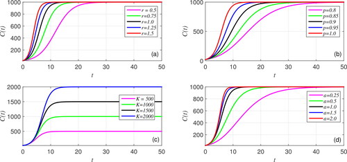
Figure 2. The corresponding daily new cases $C\prime (t)$ of Figure 1.

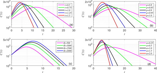
To gain more insight into the effect of each parameter, we also show in Figure 2 the curve of daily new cases $C\prime (t),$ which corresponds to Figure 1. It can be seen that the $C\prime (t)-$ curve remains symmetrical around the peak even though the value of $\widehat{r}$ or K is varied, see Figure 2(a,c). The peak value of $C\prime (t)$ increases, but the time of occurrence decreases as the value of $\widehat{r}$ increases. A similar peak behavior is also observed when we vary the value of p or a, but the $C\prime (t)-$ curve is no longer symmetrical around the peak, see Figure 2(b,d).

3. A Generalized fractional-order Richards model

3.1. Basic definitions

In this section, we consider a fractional-order version of Equation (1)(1) $$\frac{\mathit{\text{dC}}(t)}{\mathit{\text{dt}}}=C\prime (t)=\widehat{r} C{(t)}^p\left(1-{\left(\frac{C(t)}{K}\right)}^a\right),$$(1) . We begin by presenting some important definitions that correspond to the fractional-order differential equation.

Definition 3.1. (Miller & Ross, 1993) The Caputo fractional derivative of the order-$\alpha ,0<\alpha <1,$ of a function $y\in C^1$ is defined by (2) $${}^C{\mathcal{D}}_t^{\alpha }y(t)=\frac{1}{\Gamma (1-\alpha )}{\int }_0^t{(t-s)}^{-\alpha }y\prime (s)\mathit{\text{ds}},t\ge 0,$$(2)

here Γ is the Gamma function, provided that the right-hand side exists pointwise on $t\ge 0.$

Notice that, the kernel ${(t-s)}^{-\alpha }$ in Equation (2)(2) $${}^C{\mathcal{D}}_t^{\alpha }y(t)=\frac{1}{\Gamma (1-\alpha )}{\int }_0^t{(t-s)}^{-\alpha }y\prime (s)\mathit{\text{ds}},t\ge 0,$$(2) has a singularity at t = s. To avoid such singularity, Atangana-Baleanu introduced a new definition of the fractional-order derivative. In the sense of Caputo, the Atangana–Baleanu fractional-order derivative is defined as follows.

Definition 3.2. (Atangana & Baleanu, 2016) Let $0<\alpha <1,y\in C^1(a,b),$ where a < b. The Atangana–Baleanu fractional derivative in the Caputo sense of order-α (ABC sense) is given by $${}^{\mathit{\text{ABC}}}{\mathcal{D}}_t^{\alpha }f(t)=\frac{B(\alpha )}{1-\alpha }{\int }_0^t{E}_{\alpha }\left[-\frac{\alpha }{1-\alpha }{(t-s)}^{\alpha }\right]y\prime (s)\mathit{\text{ds}},$$ where $t\ge 0,$ and $E_{\alpha }(t)$ is the Mittag–Leffler function, defined by $E_{\alpha }(t)={\sum }_{n=0}^{\infty }\frac{t^n}{\Gamma (\alpha n+1)}.$ Here, $B(\alpha )$ is a normalization function, that must satisfy $B(0)=B(1)=1$ and is defined by $B(\alpha )=1-\alpha +\frac{\alpha }{\Gamma (\alpha )}.$

The Atangana–Baleanu fractional derivative in the Caputo sense is also known as the ABC fractional-order derivative. The fractional integral which corresponds to the ABC fractional-order derivative is given as follows.

Definition 3.3. (Atangana & Baleanu, 2016) The Atangana–Baleanu fractional integral of order $-\alpha$ is defined by $${}^{\mathit{\text{ABC}}}{\mathcal{I}}_t^{\alpha }f(t)=\frac{1-\alpha }{B(\alpha )}f(t)+\frac{\alpha }{\Gamma (\alpha )B(\alpha )}{\int }_0^t{(t-s)}^{\alpha -1}f(s)\mathit{\text{ds}}.$$

3.2 A generalized Caputo fractional-order Richards model

The GRM presented in Section 2 is in the form of a first-order differential equation and thus it does not consider memory effect. In this section, we propose a generalized fractional-order Richards model to account for the memory effect. A fractional-order model is achieved by replacing the first-order derivative in Equation (1)(1) $$\frac{\mathit{\text{dC}}(t)}{\mathit{\text{dt}}}=C\prime (t)=\widehat{r} C{(t)}^p\left(1-{\left(\frac{C(t)}{K}\right)}^a\right),$$(1) with a fractional-order derivative and then taking care of model homogeneity of dimension. By using the Caputo operator, we get a generalized Caputo fractional-order Richards model (GCFRM) (3) $${}^C{\mathcal{D}}_t^{\alpha }C(t)=\mathit{\text{rC}}{(t)}^p\left(1-{\left(\frac{C(t)}{K}\right)}^a\right),$$(3) where $C(t),t,p,K,$ and a have the same meaning as in Equation (1)(1) $$\frac{\mathit{\text{dC}}(t)}{\mathit{\text{dt}}}=C\prime (t)=\widehat{r} C{(t)}^p\left(1-{\left(\frac{C(t)}{K}\right)}^a\right),$$(1) . Here, we take $r={\widehat{r}}^{\alpha }$ to preserve the balance of dimension in the equation, where $\widehat{r}$ is also the same as in Equation (1)(1) $$\frac{\mathit{\text{dC}}(t)}{\mathit{\text{dt}}}=C\prime (t)=\widehat{r} C{(t)}^p\left(1-{\left(\frac{C(t)}{K}\right)}^a\right),$$(1) . The solution of Equation (3)(3) $${}^C{\mathcal{D}}_t^{\alpha }C(t)=\mathit{\text{rC}}{(t)}^p\left(1-{\left(\frac{C(t)}{K}\right)}^a\right),$$(3) can be expressed in the form of a nonlinear Volterra integral equation (4) $$C(t)=C_0+\frac{1}{\Gamma (\alpha )}{\int }_0^t{(t-s)}^{\alpha -1}f(s,C(s))\mathit{\text{ds}},$$(4) where $f(s,C(s))=\mathit{\text{rC}}{(s)}^p\left(1-{(\frac{C(s)}{K})}^a\right)$ and $C(0)=C_0.$ We consider Equation (3)(3) $${}^C{\mathcal{D}}_t^{\alpha }C(t)=\mathit{\text{rC}}{(t)}^p\left(1-{\left(\frac{C(t)}{K}\right)}^a\right),$$(3) for $t\in [0,T],T>0.$ To determine numerical solutions, the domain $[0,T]$ is discretized using a uniform grid $t_m=\mathit{\text{mh}},m=0,1,\dots ,N$ where $h=T/N$ with N is an arbitrary positive integer. Following Diethelm, Ford, and Freed (2002), we implement an Adams–Bashforth–Moulton predictor–corrector method. The predictor scheme is derived by approximating the integral in Equation (4)(4) $$C(t)=C_0+\frac{1}{\Gamma (\alpha )}{\int }_0^t{(t-s)}^{\alpha -1}f(s,C(s))\mathit{\text{ds}},$$(4) using the rectangle rule to get the fractional Adams–Bashforth predictor method (5) $$C_{m+1}^{*}=C_0+\frac{1}{\Gamma (\alpha )}\sum _{j=0}^m{a}_{j,m+1}f(t_j,C_j),$$(5)

where $C_j=C(t_j)$ and $$a_{j,m+1}=\frac{h^{\alpha }}{\alpha }\left({(m-j+1)}^{\alpha }-{(m-j)}^{\alpha }\right).$$

By applying a similar procedure, but the integral in the right hand side of Equation (4)(4) $$C(t)=C_0+\frac{1}{\Gamma (\alpha )}{\int }_0^t{(t-s)}^{\alpha -1}f(s,C(s))\mathit{\text{ds}},$$(4) is replaced by the trapezoidal quadrature rule, we get the fractional Adams-Moulton corrector method (6) $$C_{m+1}=C_0+\frac{h^{\alpha }}{\Gamma (\alpha +2)}\left(f(t_{m+1},C_{m+1}^{*})+\sum _{j=0}^m{b}_{j,m+1}f(t_j,C_j)\right),$$(6) where $$b_{j,m+1}=\{\begin{array}{lll}{m}^{\alpha +1}-(m-\alpha ){(m+1)}^{\alpha }& \text{if}& j=0,\\ {(m-j+2)}^{\alpha +1}+{(m-j)}^{\alpha +1}-2{(m-j+1)}^{\alpha +1}& \text{if}& 1\le j\le m,\\ 1& \text{if}& j=m+1.\end{array}$$

3.3. A generalized ABC fractional-order Richards model

To get a fractional-order Richards model involving the Atangana–Baleanu operator in the Caputo sense (GABCFRM), we replace the first-order derivative in Equation (1)(1) $$\frac{\mathit{\text{dC}}(t)}{\mathit{\text{dt}}}=C\prime (t)=\widehat{r} C{(t)}^p\left(1-{\left(\frac{C(t)}{K}\right)}^a\right),$$(1) with the ABC fractional-order derivative as follow (7) $${}^{\mathit{\text{ABC}}}{\mathcal{D}}_t^{\alpha }C(t)=\mathit{\text{rC}}{(t)}^p\left(1-{\left(\frac{C(t)}{K}\right)}^a\right).$$(7)

All parameters and C(t) are the same as in Equation (3)(3) $${}^C{\mathcal{D}}_t^{\alpha }C(t)=\mathit{\text{rC}}{(t)}^p\left(1-{\left(\frac{C(t)}{K}\right)}^a\right),$$(3) . The solution of Equation (7)(7) $${}^{\mathit{\text{ABC}}}{\mathcal{D}}_t^{\alpha }C(t)=\mathit{\text{rC}}{(t)}^p\left(1-{\left(\frac{C(t)}{K}\right)}^a\right).$$(7) in the form of a Volterra integral equation is given by (8) $$C(t)=C_0+\frac{1-\alpha }{B(\alpha )}f(t,C(t))+\frac{\alpha }{\Gamma (\alpha )B(\alpha )}{\int }_0^t{(t-s)}^{\alpha -1}f(s,C(s))\mathit{\text{ds}},$$(8) where $f(s,C(s))=\mathit{\text{rC}}{(s)}^p\left(1-{(\frac{C(s)}{K})}^a\right).$ Using the same procedure as in Baleanu, Jajarmi, and Hajipour (2018), we also derive a fractional-order Adams–Bashforth–Moulton predictor–corrector method for Equation (7)(7) $${}^{\mathit{\text{ABC}}}{\mathcal{D}}_t^{\alpha }C(t)=\mathit{\text{rC}}{(t)}^p\left(1-{\left(\frac{C(t)}{K}\right)}^a\right).$$(7) . In fact, the idea of this method is the same as the predictor–corrector method Equations (5)(5) $$C_{m+1}^{*}=C_0+\frac{1}{\Gamma (\alpha )}\sum _{j=0}^m{a}_{j,m+1}f(t_j,C_j),$$(5) and (6)(6) $$C_{m+1}=C_0+\frac{h^{\alpha }}{\Gamma (\alpha +2)}\left(f(t_{m+1},C_{m+1}^{*})+\sum _{j=0}^m{b}_{j,m+1}f(t_j,C_j)\right),$$(6) , namely by approximating the integral in the right hand side of Equation (8)(8) $$C(t)=C_0+\frac{1-\alpha }{B(\alpha )}f(t,C(t))+\frac{\alpha }{\Gamma (\alpha )B(\alpha )}{\int }_0^t{(t-s)}^{\alpha -1}f(s,C(s))\mathit{\text{ds}},$$(8) . If the integral is calculated using the rectangle rule, then we have the following fractional Adams–Bashforth predictor scheme (9) $$C_{m+1}^{*}=C_0+\frac{h^{\alpha }}{\Gamma (\alpha )B(\alpha )}\sum _{j=0}^m{\widehat{a}}_{m+1,j}f(t_j,C_j),$$(9) where $${\widehat{a}}_{m+1,j}=\{\begin{array}{ccc}{(m-j+1)}^{\alpha }-{(m-j)}^{\alpha }& ,& j=0,1,\dots ,m-1\\ 1+\frac{(1-\alpha )\Gamma (\alpha )}{h^{\alpha }}& ,& j=m.\end{array}$$

If the integral in Equation (8)(8) $$C(t)=C_0+\frac{1-\alpha }{B(\alpha )}f(t,C(t))+\frac{\alpha }{\Gamma (\alpha )B(\alpha )}{\int }_0^t{(t-s)}^{\alpha -1}f(s,C(s))\mathit{\text{ds}},$$(8) is approximated by the trapezoidal quadrature method, then we obtain the fractional Adams–Moulton corrector scheme (10) $$C_{m+1}=C_0+\frac{\alpha h^{\alpha }}{\Gamma (\alpha +2)B(\alpha )}(\left(1+\frac{(1-\alpha )\Gamma (\alpha +2)}{\alpha h^{\alpha }}\right)f(t_{m+1},C_{m+1}^{*})+\sum _{j=0}^m{\widehat{b}}_{m+1,j}f(t_j,C_j)),$$(10) where $${\widehat{b}}_{m+1,j}=\{\begin{array}{lll}-(m-\alpha ){(m+1)}^{\alpha +1}+m^{\alpha +1}& \text{if}& j=0,\\ {(m-j+2)}^{\alpha +1}+{(m-j)}^{\alpha +1}-2{(m-j+1)}^{\alpha +1}& \text{if}& 1\le j\le m,\\ 1& \text{if}& j=m+1.\end{array}$$

3.4. Numerical results

This Subsection presents numerical solutions of both Caputo fractional-order generalized Richards model Equation (3)(3) $${}^C{\mathcal{D}}_t^{\alpha }C(t)=\mathit{\text{rC}}{(t)}^p\left(1-{\left(\frac{C(t)}{K}\right)}^a\right),$$(3) and Atangana–Baleanu fractional-order generalized Richards model Equation (7)(7) $${}^{\mathit{\text{ABC}}}{\mathcal{D}}_t^{\alpha }C(t)=\mathit{\text{rC}}{(t)}^p\left(1-{\left(\frac{C(t)}{K}\right)}^a\right).$$(7) . The numerical solutions of Equation (3)(3) $${}^C{\mathcal{D}}_t^{\alpha }C(t)=\mathit{\text{rC}}{(t)}^p\left(1-{\left(\frac{C(t)}{K}\right)}^a\right),$$(3) are obtained by applying the predictor–corrector scheme Equation (5)(5) $$C_{m+1}^{*}=C_0+\frac{1}{\Gamma (\alpha )}\sum _{j=0}^m{a}_{j,m+1}f(t_j,C_j),$$(5) and (6)(6) $$C_{m+1}=C_0+\frac{h^{\alpha }}{\Gamma (\alpha +2)}\left(f(t_{m+1},C_{m+1}^{*})+\sum _{j=0}^m{b}_{j,m+1}f(t_j,C_j)\right),$$(6) , while those of Equation (7)(7) $${}^{\mathit{\text{ABC}}}{\mathcal{D}}_t^{\alpha }C(t)=\mathit{\text{rC}}{(t)}^p\left(1-{\left(\frac{C(t)}{K}\right)}^a\right).$$(7) are obtained by implementing the predictor–corrector scheme Equation (9)(9) $$C_{m+1}^{*}=C_0+\frac{h^{\alpha }}{\Gamma (\alpha )B(\alpha )}\sum _{j=0}^m{\widehat{a}}_{m+1,j}f(t_j,C_j),$$(9) and (10)(10) $$C_{m+1}=C_0+\frac{\alpha h^{\alpha }}{\Gamma (\alpha +2)B(\alpha )}(\left(1+\frac{(1-\alpha )\Gamma (\alpha +2)}{\alpha h^{\alpha }}\right)f(t_{m+1},C_{m+1}^{*})+\sum _{j=0}^m{\widehat{b}}_{m+1,j}f(t_j,C_j)),$$(10) . To study the influence of the parameters, we performed some simulations with different parameter values and the order of the fractional derivative.

In Figures 3 and 4 we compare the numerical results of the Caputo fractional-order generalized Richards model (left-panel) and the Atangana–Baleanu in the Caputo sense (ABC) fractional-order generalized Richards model (right-panel) with $C(0)=20$ for different order of derivative $\alpha =0.6,0.7,0.8,0.9,1.0$ and various parameter values.

Figure 3. The cumulative number of cases C(t) obtained by the Caputo fractional-order generalized Richards model (left-panel) and the Atangana-Baleanu in the Caputo sense (ABC) fractional-order generalized Richards model (right-panel) with parameter values (a,b) $r=p=a=1,K=1000;$ (c,d) $r=0.1,p=a=1,K=1000;$ (e,f) $r=1,p=0.5,a=1,K=1000;$ and (g,h) $r=1,p=1,a=2,K=1000.$ The arrow shows increasing values of $\alpha =0.6,0.7,0.8,0.9,$ and 1.0.

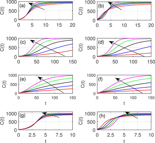
Figure 4. The corresponding daily new cases $C\prime (t)$ obtained by the Caputo fractional-order generalized Richards model (left-panel) and the Atangana-Baleanu in the Caputo sense (ABC) fractional-order generalized Richards model (right-panel) with parameter values (a,b) $r=p=a=1,K=1000;$ (c,d) $r=0.1,p=a=1,K=1000;$ (e,f) $r=1,p=0.5,a=1,K=1000;$ and (g,h) $r=1,p=1,a=2,K=1000.$ The arrow shows increasing values of $\alpha =0.6,0.7,0.8,0.9,$ and 1.0.

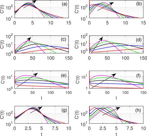
The numerical results of C(t) and $C\prime (t)$ tend towards the model with the first-order derivative case as $\alpha \to 1.$ However, the convergence of the solutions to the final size of the epidemic (K) slows down as the value of α decreases. This shows that the stabilization time of response decreases with decreasing α. Figures 3(a,b) and 4(a,b) depict the numerical solutions for the case with parameter values $r=p=a=1,K=1000.$ For this case, we observe that the initial growth rates for the model with the Caputo operator are very similar for all α. On the contrary, the model with the ABC operator has different type of initial growth rate for different values of α. The peak of $C\prime (t)$ obtained by the fractional model with the Caputo operator increases and the time of appearance increases slightly with increasing α. Such behavior is more pronounced by the fractional model with the ABC operator. Similar properties of C(t) and $C\prime (t)$ are also observed when we increase the value of a such that a = 2, see Figures 3(g,h) and 4(g,h).

If we reduce the intrinsic growth rate so that r = 1 while keeping $p=a=1,K=1000,$ then the increase in the order of the fractional derivative $(\alpha )$ causes a shortening of the sigmoidal behavior of the curve C(t) and the point of inflection (or the peak of $C\prime (t)$) appears faster for both fractional-order models with the Caputo operator and ABC operator. Variations in the value of α also affect the asymptotic behavior of both C(t) and $C\prime (t),$ which indicates that growth is faster and the asymptote achieved is higher as $\alpha \to 1;$ see Figures 3(c,d) and 4(c,d). We observe very similar behavior if we take $r=1,p=0.5,a=1,K=1000,$ see Figures 3(e,f) and 4(e,f).

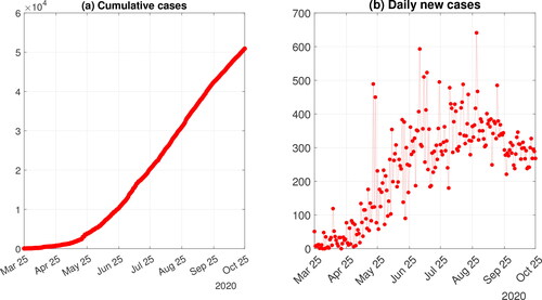
4. Implementation to COVID-19 data in East Java, Indonesia

In this section, we apply the fractional-order GRM to COVID-19 data in East Java Province, Indonesia, from March 25 until October 31, 2020. This data was taken from the official website of the Indonesian National Task Force for the Acceleration of COVID-19 Response, www.covid19.go.id. The cumulative number of cases and the daily new cases of COVID-19 in East Java are shown in Figure 5. The daily data of a cumulative number of cases are fitted to the GCFRM (3)(3) $${}^C{\mathcal{D}}_t^{\alpha }C(t)=\mathit{\text{rC}}{(t)}^p\left(1-{\left(\frac{C(t)}{K}\right)}^a\right),$$(3) and the GABCFRM (7)(7) $${}^{\mathit{\text{ABC}}}{\mathcal{D}}_t^{\alpha }C(t)=\mathit{\text{rC}}{(t)}^p\left(1-{\left(\frac{C(t)}{K}\right)}^a\right).$$(7) to find the model parameters which minimize the sum of the squared residual between the numerical solutions of each fractional-order GRM and the related data. Here, we estimate the model parameters via a nonlinear least-square method, namely by applying a built-in MATLAB function lsqcurvefit. The initial guess values of the parameters are $r=0.3,p=1,K=40000,$ and $a=0.1.$ The model calibration to estimate the model parameters is performed for three different data periods, i.e. March 25—May 24, 2020 (61 d), March 25—Jul 24, 2020 (122 d) and March 25 – Oct 21, 2020 (211 d). According to Du et al. (2013), the order of fractional derivative, that is α, can be considered as an index of memory. To investigate how fractional GRM behaves over various fractional-orders of the derivative with the inclusion of memory effects, we estimate the parameters of the fractional GRM using $\alpha =0.95,0.9,0.85,0.8.$ Thus, the fractional-order derivative is considered as an additional degree of freedom in the model.

Figure 5. Cumulative number of COVID-19 cases (left-panel) and daily new cases of COVID-19 (right-panel) in East Java Province, Indonesia.

The estimated parameters based on the GCFRM and GABCFRM for each data period are respectively shown in Tables 1 and 2. Figures 6 and 7 show respectively the fitting curve resulted from the GCFRM (3)(3) $${}^C{\mathcal{D}}_t^{\alpha }C(t)=\mathit{\text{rC}}{(t)}^p\left(1-{\left(\frac{C(t)}{K}\right)}^a\right),$$(3) and the GABCFRM (7)(7) $${}^{\mathit{\text{ABC}}}{\mathcal{D}}_t^{\alpha }C(t)=\mathit{\text{rC}}{(t)}^p\left(1-{\left(\frac{C(t)}{K}\right)}^a\right).$$(7) . We also present 10-day ahead forecasts for each simulation. For comparison, we also plot the fitting curve obtained from the GRM (1)(1) $$\frac{\mathit{\text{dC}}(t)}{\mathit{\text{dt}}}=C\prime (t)=\widehat{r} C{(t)}^p\left(1-{\left(\frac{C(t)}{K}\right)}^a\right),$$(1) , i.e. when α = 1, and the cumulative confirmed cases data; see left panels. Here, the cumulative confirmed cases are plotted in red markers (data used for calibration) and blue markers (data for comparison of forescasting results). In the right panels of Figures 6 and 7, we compare the corresponding curve fitting of daily new cases $C\prime (t)$ with the confirmed daily new cases. It is seen that in the scale of Figures 6 and 7, the predictions of cumulative cases C(t) by the GRM (1)(1) $$\frac{\mathit{\text{dC}}(t)}{\mathit{\text{dt}}}=C\prime (t)=\widehat{r} C{(t)}^p\left(1-{\left(\frac{C(t)}{K}\right)}^a\right),$$(1) , the GCFRM (3)(3) $${}^C{\mathcal{D}}_t^{\alpha }C(t)=\mathit{\text{rC}}{(t)}^p\left(1-{\left(\frac{C(t)}{K}\right)}^a\right),$$(3) and the GABCFRM (7)(7) $${}^{\mathit{\text{ABC}}}{\mathcal{D}}_t^{\alpha }C(t)=\mathit{\text{rC}}{(t)}^p\left(1-{\left(\frac{C(t)}{K}\right)}^a\right).$$(7) for three different data periods are equally good, both during calibration and forecasting. Although there is dispersion in the data, the GRM (1)(1) $$\frac{\mathit{\text{dC}}(t)}{\mathit{\text{dt}}}=C\prime (t)=\widehat{r} C{(t)}^p\left(1-{\left(\frac{C(t)}{K}\right)}^a\right),$$(1) , the GCFRM (3)(3) $${}^C{\mathcal{D}}_t^{\alpha }C(t)=\mathit{\text{rC}}{(t)}^p\left(1-{\left(\frac{C(t)}{K}\right)}^a\right),$$(3) and the GABCFRM (7)(7) $${}^{\mathit{\text{ABC}}}{\mathcal{D}}_t^{\alpha }C(t)=\mathit{\text{rC}}{(t)}^p\left(1-{\left(\frac{C(t)}{K}\right)}^a\right).$$(7) are able to predict the data’s typical behavior, which includes both increasing and decreasing behaviors as well as strong agreement between the inflection points and also the occurrence time of maximum cases.

Figure 6. (a–f) Numerical solutions of the fitted GCFRM (3)(3) $${}^C{\mathcal{D}}_t^{\alpha }C(t)=\mathit{\text{rC}}{(t)}^p\left(1-{\left(\frac{C(t)}{K}\right)}^a\right),$$(3) compared to the confirmed COVID-19 data from east java. In the left panel, the fitted curves C(t) of the GCFRM (3)(3) $${}^C{\mathcal{D}}_t^{\alpha }C(t)=\mathit{\text{rC}}{(t)}^p\left(1-{\left(\frac{C(t)}{K}\right)}^a\right),$$(3) using three different data periods: namely (a) March 25 – May 24, 2020 (61 d), (c) march 25 – Jul 24, 2020 (122 d) and (e) march 25 – Oct 21, 2020 (211 d), are compared to the cumulative confirmed cases; while the right panels show the comparison between the corresponding fitted $C\prime (t)$ which are calculated numerically and the confirmed new daily cases.

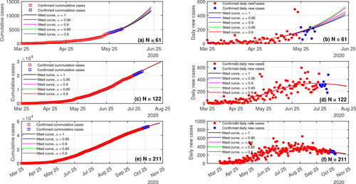
Figure 7. (a–f) Numerical solutions of the fitted GABCFRM (7)(7) $${}^{\mathit{\text{ABC}}}{\mathcal{D}}_t^{\alpha }C(t)=\mathit{\text{rC}}{(t)}^p\left(1-{\left(\frac{C(t)}{K}\right)}^a\right).$$(7) compared to the confirmed COVID-19 data from east java. In the left panel, the fitted curves C(t) of the GABCFRM (7)(7) $${}^{\mathit{\text{ABC}}}{\mathcal{D}}_t^{\alpha }C(t)=\mathit{\text{rC}}{(t)}^p\left(1-{\left(\frac{C(t)}{K}\right)}^a\right).$$(7) using three different data periods: namely (a) March 25 – May 24, 2020 (61 d), (c) march 25 – Jul 24, 2020 (122 d) and (e) march 25 – Oct 21, 2020 (211 d), are compared to the cumulative confirmed cases; while the right panels show the comparison between the corresponding fitted $C\prime (t)$ which are calculated numerically and the confirmed new daily cases.

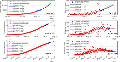
Table 1. Estimated value of parameter based on the GCFRM (3)(3) $${}^C{\mathcal{D}}_t^{\alpha }C(t)=\mathit{\text{rC}}{(t)}^p\left(1-{\left(\frac{C(t)}{K}\right)}^a\right),$$(3) for different value of α. Notice that α = 1 corresponds to the first order GRM (1)(1) $$\frac{\mathit{\text{dC}}(t)}{\mathit{\text{dt}}}=C\prime (t)=\widehat{r} C{(t)}^p\left(1-{\left(\frac{C(t)}{K}\right)}^a\right),$$(1) .

Number of Data	Parameter	α = 1	$\alpha =0.95$	$\alpha =0.9$	$\alpha =0.85$	$\alpha =0.8$
61	r	0.3487	0.1737	0.2092	0.2165	0.1952
	p	0.9458	0.9115	0.8634	0.8790	0.9718
	K	439,254	483,057	498,267	498,550	484,579
	a	0.0801	0.2275	0.9956	0.9971	0.1840
122	r	0.2260	0.1575	0.1652	0.1732	0.1821
	p	0.9525	0.9415	0.9526	0.9659	0.9789
	K	48,508	50,339	53,315	56,782	60,623
	a	0.2206	0.2931	0.2980	0.2940	0.2900
211	r	0.3891	0.2723	0.2710	0.2708	0.2721
	p	0.9072	0.9280	0.9405	0.9518	0.9618
	K	76,643	80,878	85,443	90,488	96,097
	a	0.1387	0.1282	0.1376	0.1486	0.1619

Table 2. Estimated value of parameter based on the GABCFRM (7)(7) $${}^{\mathit{\text{ABC}}}{\mathcal{D}}_t^{\alpha }C(t)=\mathit{\text{rC}}{(t)}^p\left(1-{\left(\frac{C(t)}{K}\right)}^a\right).$$(7) for different value of α. Notice that α = 1 corresponds to the first order GRM (1)(1) $$\frac{\mathit{\text{dC}}(t)}{\mathit{\text{dt}}}=C\prime (t)=\widehat{r} C{(t)}^p\left(1-{\left(\frac{C(t)}{K}\right)}^a\right),$$(1) .

Number of Data	Parameter	α = 1	$\alpha =0.95$	$\alpha =0.9$	$\alpha =0.85$	$\alpha =0.8$
61	r	0.3487	0.1739	0.1851	0.2159	0.1918
	p	0.9458	0.9151	0.9507	0.8861	0.9828
	K	439,254	478,176	452,523	499,644	442,946
	a	0.0801	0.2225	0.1685	0.9999	0.1883
122	r	0.2260	0.1580	0.1653	0.1733	0.1816
	p	0.9525	0.9424	0.9569	0.9698	0.9834
	K	48,508	50,261	53,296	56,581	60,344
	a	0.2206	0.2969	0.2983	0.3053	0.3103
211	r	0.3891	0.2726	0.2567	0.2692	0.2671
	p	0.9072	0.9297	0.9316	0.9579	0.9696
	K	76,643	80,839	85,168	90,379	95,977
	a	0.1387	0.1288	0.1697	0.1509	0.1685

To be more detail, we provide a quantitative comparison between confirmed and predicted cumulative cases data by calculating the coefficient of determination $(R^2),$ see Table 3, and the root mean square error (RMSE), see Tables 4 and 5. It is found that all methods have a very high coefficient of determination; confirming that the GRM (1)(1) $$\frac{\mathit{\text{dC}}(t)}{\mathit{\text{dt}}}=C\prime (t)=\widehat{r} C{(t)}^p\left(1-{\left(\frac{C(t)}{K}\right)}^a\right),$$(1) , the GCFRM (3)(3) $${}^C{\mathcal{D}}_t^{\alpha }C(t)=\mathit{\text{rC}}{(t)}^p\left(1-{\left(\frac{C(t)}{K}\right)}^a\right),$$(3) and the GABCFRM (7)(7) $${}^{\mathit{\text{ABC}}}{\mathcal{D}}_t^{\alpha }C(t)=\mathit{\text{rC}}{(t)}^p\left(1-{\left(\frac{C(t)}{K}\right)}^a\right).$$(7) perform well. However, the GABCFRM (7)(7) $${}^{\mathit{\text{ABC}}}{\mathcal{D}}_t^{\alpha }C(t)=\mathit{\text{rC}}{(t)}^p\left(1-{\left(\frac{C(t)}{K}\right)}^a\right).$$(7) typically offers the best prediction because it has the highest R². It is also observed that the more data used in calibration, the higher the coefficient of determination. Furthermore, the RMSE of the calibrating of the cumulative number of cases using three different data periods suggests that the fractional-order GRM, with both Caputo and ABC operators, may perform better than the first-order GRM. In this case, the GABCFRM (7)(7) $${}^{\mathit{\text{ABC}}}{\mathcal{D}}_t^{\alpha }C(t)=\mathit{\text{rC}}{(t)}^p\left(1-{\left(\frac{C(t)}{K}\right)}^a\right).$$(7) is the best because it has the smallest RMSE value for a certain value of α. However, when performing the 10-day forecast of cumulative number of cases using the data period March 25—May 24 (61 d), the GCFRM (3)(3) $${}^C{\mathcal{D}}_t^{\alpha }C(t)=\mathit{\text{rC}}{(t)}^p\left(1-{\left(\frac{C(t)}{K}\right)}^a\right),$$(3) with $\alpha =0.95$ has the smallest RMSE than other models. When using data periods March 25—Jul 24, 2020 (122 d) and March 25 - Oct 21, 2020 (211 d), the smallest RMSE of the 10-day estimates of the cumulative number of cases are given by the GABCFRM with $\alpha =0.8,$ and the GRM (1)(1) $$\frac{\mathit{\text{dC}}(t)}{\mathit{\text{dt}}}=C\prime (t)=\widehat{r} C{(t)}^p\left(1-{\left(\frac{C(t)}{K}\right)}^a\right),$$(1) , respectively. In Tables 6 and 7 we also show respectively the RMSE of the calibrating and the 10-day forecast of daily new cases. It is observed that all models, namely the GRM (1)(1) $$\frac{\mathit{\text{dC}}(t)}{\mathit{\text{dt}}}=C\prime (t)=\widehat{r} C{(t)}^p\left(1-{\left(\frac{C(t)}{K}\right)}^a\right),$$(1) , the GCFRM (3)(3) $${}^C{\mathcal{D}}_t^{\alpha }C(t)=\mathit{\text{rC}}{(t)}^p\left(1-{\left(\frac{C(t)}{K}\right)}^a\right),$$(3) , and the GABCFRM (7)(7) $${}^{\mathit{\text{ABC}}}{\mathcal{D}}_t^{\alpha }C(t)=\mathit{\text{rC}}{(t)}^p\left(1-{\left(\frac{C(t)}{K}\right)}^a\right).$$(7) have comparable performance. Based on the above discussion, we can say that the fractional-order GRM with ABC operator (7)(7) $${}^{\mathit{\text{ABC}}}{\mathcal{D}}_t^{\alpha }C(t)=\mathit{\text{rC}}{(t)}^p\left(1-{\left(\frac{C(t)}{K}\right)}^a\right).$$(7) generally has the best performance when applied to COVID-19 data in East Java, Indonesia.

Table 3. Coefficient of determination for the calibration of cumulative number of cases.

	GCFRM				GABCFRM				GRM
Number of Data	$\alpha =0.95$	$\alpha =0.9$	$\alpha =0.85$	$\alpha =0.8$	$\alpha =0.95$	$\alpha =0.9$	$\alpha =0.85$	$\alpha =0.8$	α = 1
61	0.9803	0.9815	0.9817	0.9804	0.9804	0.9807	0.9824	0.9817	0.9798
122	0.9992	0.9991	0.9990	0.9988	0.9992	0.9992	0.9992	0.9992	0.9992
211	0.9998	0.9998	0.9998	0.9998	0.9998	0.9998	0.9998	0.9998	0.9998

Table 4. RMSE of the calibrating of cumulative number of cases.

	GCFRM				GABCFRM				GRM
Number of Data	$\alpha =0.95$	$\alpha =0.9$	$\alpha =0.85$	$\alpha =0.8$	$\alpha =0.95$	$\alpha =0.9$	$\alpha =0.85$	$\alpha =0.8$	α = 1
61	125.8574	121.7239	122.1593	126.1321	121.4933	119.3389	124.7614	125.8595	127.8081
122	206.5081	187.9044	177.6321	173.1599	171.6956	171.7629	171.8656	171.9872	172.2141
211	286.4225	255.843	239.703	233.054	232.1349	231.7616	232.2087	231.6902	232.2173

Table 5. RMSE of the 10-day forecast of cumulative number of cases.

	GCFRM				GABCFRM				GRM
Number of Data	$\alpha =0.95$	$\alpha =0.9$	$\alpha =0.85$	$\alpha =0.8$	$\alpha =0.95$	$\alpha =0.9$	$\alpha =0.85$	$\alpha =0.8$	α = 1
61	143.714	159.0928	163.1623	193.354	179.651	174.3873	198.8365	204.8918	224.3442
122	466.8341	395.483	337.4354	293.7349	264.0404	262.6498	261.4765	260.0616	270.2056
211	345.6237	245.1908	161.0831	90.8242	156.604	124.8663	89.6419	63.2994	38.1256

Table 6. RMSE of the calibrating of daily new cases.

	GCFRM				GABCFRM				GRM
Number of Data	$\alpha =0.95$	$\alpha =0.9$	$\alpha =0.85$	$\alpha =0.8$	$\alpha =0.95$	$\alpha =0.9$	$\alpha =0.85$	$\alpha =0.8$	α = 1
61	65.9749	65.8419	66.0458	66.4974	66.1704	65.9621	66.4513	66.5313	66.7344
122	79.7167	79.6992	79.6889	79.6843	79.6845	79.6832	79.6827	79.6820	79.6898
211	73.3511	73.3364	73.3268	73.3208	73.3747	73.3558	73.3425	73.3274	73.3192

Table 7. RMSE of the 10-day forecast of daily new cases.

	GCFRM				GABCFRM				GRM
Number of Data	$\alpha =0.95$	$\alpha =0.9$	$\alpha =0.85$	$\alpha =0.8$	$\alpha =0.95$	$\alpha =0.9$	$\alpha =0.85$	$\alpha =0.8$	α = 1
61	73.4206	77.4194	74.6662	68.07	71.5193	76.2984	68.4867	67.8209	65.8264
122	78.0984	77.9801	77.851	77.7871	77.8804	77.8466	77.8178	77.7527	78.0831
211	23.9375	23.3953	22.9779	22.7332	24.1934	23.5084	22.9651	22.7311	22.7137

It was noticed previously that the operator of the Caputo fractional-order derivative has a singular kernel and the solution of the GCFRM (3)(3) $${}^C{\mathcal{D}}_t^{\alpha }C(t)=\mathit{\text{rC}}{(t)}^p\left(1-{\left(\frac{C(t)}{K}\right)}^a\right),$$(3) can be represented by the nonlinear Volterra integral Equation (4)(4) $$C(t)=C_0+\frac{1}{\Gamma (\alpha )}{\int }_0^t{(t-s)}^{\alpha -1}f(s,C(s))\mathit{\text{ds}},$$(4) . However, the GCFRM (3)(3) $${}^C{\mathcal{D}}_t^{\alpha }C(t)=\mathit{\text{rC}}{(t)}^p\left(1-{\left(\frac{C(t)}{K}\right)}^a\right),$$(3) provides good calibration and forecasting results on COVID-19. This indicates that the Volterra integral Equation (4)(4) $$C(t)=C_0+\frac{1}{\Gamma (\alpha )}{\int }_0^t{(t-s)}^{\alpha -1}f(s,C(s))\mathit{\text{ds}},$$(4) is integrable. Nonetheless, we remark that the existence and uniqueness of the solution to the GCFRM (3)(3) $${}^C{\mathcal{D}}_t^{\alpha }C(t)=\mathit{\text{rC}}{(t)}^p\left(1-{\left(\frac{C(t)}{K}\right)}^a\right),$$(3) is still an open problem. We also notice that in contrast to the first-order GRM (1)(1) $$\frac{\mathit{\text{dC}}(t)}{\mathit{\text{dt}}}=C\prime (t)=\widehat{r} C{(t)}^p\left(1-{\left(\frac{C(t)}{K}\right)}^a\right),$$(1) , the GCFRM (3)(3) $${}^C{\mathcal{D}}_t^{\alpha }C(t)=\mathit{\text{rC}}{(t)}^p\left(1-{\left(\frac{C(t)}{K}\right)}^a\right),$$(3) and the GABCFRM (7)(7) $${}^{\mathit{\text{ABC}}}{\mathcal{D}}_t^{\alpha }C(t)=\mathit{\text{rC}}{(t)}^p\left(1-{\left(\frac{C(t)}{K}\right)}^a\right).$$(7) provide an additional degree of freedom, i.e. via selecting the order of fractional derivative $(\alpha ).$ With this in mind, several data fittings using various α have been carried out. It is shown that different values of α lead to different values of calibration RMSE. We recommend that the order of fractional derivative $(\alpha )$ is also optimized, that is, by including $(\alpha )$ as a parameter to be estimated.

5. Conclusions

We have proposed a fractional-order generalized Richards model. For the proposed model, we consider the Caputo fractional operator into the generalized Richards model. In the Caputo operator, there is a condition such that the kernel is singular. Hence, we also consider the Atangana–Baleanu operator in the Caputo sense (ABC), involving the Mittag–Leffler function as a kernel to the model, which avoids the singularity in the Caputo operator. The solutions of the models are obtained numerically by implementing the predictor-corrector schemes based on the derivation of the Adam-Bashforth–Moutlon method. The numerical results show that the convergence of fractional-order models slows down as derivative order decreases. Furthermore, the behavior of the fractional-order model with an ABC operator is more pronounced than that with a Caputo operator for different orders.

We have employed the proposed models to COVID-19 data via the nonlinear least-squares method, such that the coefficient of determination (R²) and the root mean squared error (RMSE) are obtained for different orders and operator types. Regardless of the number of data, the fractional-order model with the ABC operator has the highest coefficient of determination, which typically offers the best prediction. The fractional-order model with the ABC operator has the best performance due to the lowest RMSE generally in calibration and forecasting of COVID-19 cases. For future studies, we suggest that the order of the fractional derivative is also included as a parameter to be estimated.

Disclosure statement

No potential conflict of interest was reported by the authors.

Additional information

Funding

This research was funded by the Faculty of Mathematics and Natural Sciences (FMIPA) through Public Funds DPA (Dokumen Pelaksanaan Anggaran) Perguruan Tinggi Berbadan Hukum (PTNBH) University of Brawijaya and based on FMIPA Professor Grant Contract No. [3084.19/UN10.F09/PN/2022].

References

- Abdeljawad, T., Al-Mdallal, Q. M., & Jarad, F. (2019). Fractional logistic models in the frame of fractional operators generated by conformable derivatives. Chaos, Solitons & Fractals, 119, 94–101. doi:10.1016/j.chaos.2018.12.015
- Abdeljawad, T., Hajji, M. A., Al-Mdallal, Q. M., & Jarad, F. (2020). Analysis of some generalized ABC–fractional logistic models. Alexandria Engineering Journal, 59(4), 2141–2148. doi:10.1016/j.aej.2020.01.030
- Ali, A., Ur Rahmamn, M., Shah, Z., Kumam, P., & Adnan. (2022). Investigation of a time-fractional covid-19 mathematical model with singular kernel. Advances in Continuous and Discrete models, 2022(1), 34. doi:10.1186/s13662-022-03701-z
- Alrabaiah, H., Arfan, M., Shah, K., Mahariq, I., & Ullah, A. (2021). A comparative study of spreading of novel corona virus disease by using fractional order modified SEIR model. Alexandria Engineering Journal, 60(1), 573–585. doi:10.1016/j.aej.2020.09.036
- Atangana, A., & Baleanu, D. (2016). New fractional derivatives with nonlocal and non-singular kernel: Theory and application to heat transfer model. Thermal Science, 20(2), 763–769. doi:10.2298/TSCI160111018A
- Ausloos, M. (2006). The logistic map and the route to chaos: From the beginnings to modern applications. Berlin: Springer Science & Business Media.
- Baleanu, D., Jajarmi, A., & Hajipour, M. (2018). On the nonlinear dynamical systems within the generalized fractional derivatives with Mittag–Leffler kernel. Nonlinear Dynamics, 94(1), 397–414. doi:10.1007/s11071-018-4367-y
- Bürger, R., Chowell, G., & Lara-Díaz, L. Y. (2021). Measuring differences between phenomenological growth models applied to epidemiology. Mathematical Biosciences, 334, 108558. doi:10.1016/j.mbs.2021.108558
- Chowell, G. (2017). Fitting dynamic models to epidemic outbreaks with quantified uncertainty: A primer for parameter uncertainty, identifiability, and forecasts. Infectious Disease Modelling, 2(3), 379–398. doi:10.1016/j.idm.2017.08.001
- Chowell, G., & Viboud, C. (2016). Is it growing exponentially fast?–Impact of assuming exponential growth for characterizing and forecasting epidemics with initial near-exponential growth dynamics. Infectious Disease Modelling, 1(1), 71–78. doi:10.1016/j.idm.2016.07.004
- Darti, I., Habibah, U., Astutik, S., Kusumawinahyu, W. M., & Suryanto, A. (2021). Comparison of phenomenological growth models in predicting cumulative number of COVID-19 cases in East Java Province, Indonesia. Communications in Mathematical Biology and Neuroscience, 2021, 14.
- Darti, I., Musafir, R. R., Rayungsari, M., Suryanto, A., & Trisilowati. (2023). Dynamics of a fractional-order covid-19 epidemic model with quarantine and standard incidence rate. Axioms, 12(6), 591. doi:10.3390/axioms12060591
- Darti, I., Suryanto, A., Panigoro, H. S., & Susanto, H. (2021). Forecasting covid-19 epidemic in Spain and Italy using a generalized Richards model with quantified uncertainty. Communication in Biomathematical Sciences, 3(2), 90–100. doi:10.5614/cbms.2020.3.2.1
- Diethelm, K. (2010). The analysis of fractional differential equations: An application-oriented exposition using differential operators of Caputo type. Berlin: Springer Science & Business Media.
- Diethelm, K., Ford, N. J., & Freed, A. D. (2002). A predictor-corrector approach for the numerical solution of fractional differential equations. Nonlinear Dynamics, 29(1/4), 3–22. doi:10.1023/A:1016592219341
- Djeddi, N., Hasan, S., Al-Smadi, M., & Momani, S. (2020). Modified analytical approach for generalized quadratic and cubic logistic models with Caputo-Fabrizio fractional derivative. Alexandria Engineering Journal, 59(6), 5111–5122. doi:10.1016/j.aej.2020.09.041
- Du, M., Wang, Z., & Hu, H. (2013). Measuring memory with the order of fractional derivative. Scientific Reports, 3(1), 3431. doi:10.1038/srep03431
- Ezz-Eldien, S. (2018). On solving fractional logistic population models with applications. Computational and Applied Mathematics, 37(5), 6392–6409. doi:10.1007/s40314-018-0693-4
- Haidong, Q., Ur Rahman, M., Al Hazmi, S. E., Yassen, M. F., Salahshour, S., Salimi, M., & Ahmadian, A. (2023). Analysis of non-equilibrium 4d dynamical system with fractal fractional Mittag–Leffler kernel. Engineering Science and Technology, an International Journal, 37, 101319. doi:10.1016/j.jestch.2022.101319
- Jaelani, A, Fatmawati, F., & Fitri, N. D. Y. (2021). Stability analysis and optimal control of mathematical epidemic model with medical treatment. AIP Conference Proceedings, (vol. 2329, pp. 040001). AIP Publishing.
- Jafari, H., Ganji, R., Nkomo, N., & Lv, Y. (2021). A numerical study of fractional order population dynamics model. Results in Physics, 27, 104456. doi:10.1016/j.rinp.2021.104456
- Khan, Z. A., Shah, K., Abdalla, B., & Abdeljawad, T. (2023). A numerical study of complex dynamics of a Chemostat model under fractal-fractional derivative. Fractals, 31(08), 2340181. doi:10.1142/S0218348X23401813
- Li, B., Zhang, T., & Zhang, C. (2023). Investigation of financial bubble mathematical model under fractal-fractional Caputo derivative. Fractals, 31(05), 1–13. doi:10.1142/S0218348X23500500
- Miller, K. S., & Ross, B. (1993). An introduction to the fractional calculus and fractional differential equations. New York: Willy.
- Musafir, R. R., Suryanto, A., Darti, I. & Trisilowat. (2024a). Comparison of fractional-order monkeypox model with singular and non-singular kernels. Jambura Journal of Biomathematics, 5(1)
- Musafir, R. R., Suryanto, A., Darti, I., & Trisilowati. (2024b). Optimal control of a fractional-order monkeypox epidemic model with vaccination and rodents culling. Results in Control and Optimization, 14, 100381. doi:10.1016/j.rico.2024.100381
- Musafir, R. R., Suryanto, A., Darti, I., & Trisilowati. (2024c). Stability analysis of a fractional-order monkeypox epidemic model with quarantine and hospitalization. Journal of Biosafety and Biosecurity, 6(1), 34–50. doi:10.1016/j.jobb.2024.02.003
- Panigoro, H. S., Suryanto, A., Kusumawinahyu, W. M., & Darti, I. (2021). Dynamics of an eco-epidemic predator-prey model involving fractional derivatives with power-law and Mittag–Leffler kernel. Symmetry, 13(5), 785. doi:10.3390/sym13050785
- Pincheira-Brown, P., & Bentancor, A. (2021). Forecasting covid-19 infections with the semi-unrestricted generalized growth model. Epidemics, 37, 100486. doi:10.1016/j.epidem.2021.100486
- Podlubny, I. (1999). Fractional differential equations: Mathematics in science and engineering. San Diego: Academic Press.
- Rahman, M., Tabassum, S., Althobaiti, A., Althobaiti, S., & Waseem. (2024). An analysis of fractional piecewise derivative models of dengue transmission using deep neural network. Journal of Taibah University for Science, 18(1), 2340871. doi:10.1080/16583655.2024.2340871
- Rahmi, E., Darti, I., Suryanto, A., & Trisilowati, (2021). A modified Leslie–Gower model incorporating Beddington–Deangelis functional response, double Allee effect and memory effect. Fractal and Fractional, 5(3), 84. doi:10.3390/fractalfract5030084
- Richards, F. J. (1959). A flexible growth function for empirical use. Journal of Experimental Botany, 10(2), 290–301. doi:10.1093/jxb/10.2.290
- Roosa, K., Lee, Y., Luo, R., Kirpich, A., Rothenberg, R., Hyman, J. M., & Chowell, G. (2020). Short-term forecasts of the covid-19 epidemic in Guangdong and Zhejiang, China. Journal of Clinical Mmedicine, 9(2), 596. February 13–23, 2020
- Shah, K., & Abdeljawad, T. (2023). On complex fractal-fractional order mathematical modeling of co 2 emanations from energy sector. Physica Scripta, 99(1), 015226. doi:10.1088/1402-4896/ad1286
- Shah, K., Abdalla, B., Abdeljawad, T., & Alqudah, M. A. (2024). A fractal-fractional order model to study multiple sclerosis: A chronic disease. Fractals, 32(02), 2440010. doi:10.1142/S0218348X24400103
- Shah, K., Ahmad, I., Mukheimer, A., Abdeljawad, T., Jeelani, M. B., & Shafiullah. (2024). On the existence and numerical simulation of cholera epidemic model. Open Physics, 22(1), 20230165. doi:10.1515/phys-2023-0165
- Trisilowati, Darti, I., Musafir, R. R., Rayungsari, M., & Suryanto, A., & Trisilowati. (2023). Dynamics of a fractional-order covid-19 epidemic model with quarantine and standard incidence rate. Axioms, 12(6), 591. doi:10.3390/axioms12060591
- Ullah, M. S., Kabir, K. A., & Khan, M. A. H. (2023). A non-singular fractional-order logistic growth model with multi-scaling effects to analyze and forecast population growth in Bangladesh. Scientific Reports, 13(1), 20118. doi:10.1038/s41598-023-45773-1
- Viboud, C., Simonsen, L., & Chowell, G. (2016). A generalized-growth model to characterize the early ascending phase of infectious disease outbreaks. Epidemics, 15, 27–37. doi:10.1016/j.epidem.2016.01.002
- Wu, K., Darcet, D., Wang, Q., & Sornette, D. (2020). Generalized logistic growth modeling of the covid-19 outbreak: Comparing the dynamics in the 29 provinces in china and in the rest of the world. Nonlinear Dynamics, 101(3), 1561–1581. doi:10.1007/s11071-020-05862-6
- Zhang, L., Rahman, M. U., Ahmad, S., Riaz, M. B., & Jarad, F. (2022). Dynamics of fractional order delay model of coronavirus disease. AIMS Mathematics, 7(3), 4211–4232. doi:10.3934/math.2022234