The real fixed points of two-parameter family of functions bx−1xm

Abstract

In this paper, we delve into the investigation of real fixed points of a two-parameter family of functions defined as $f_{\alpha ,m}(x)=\alpha \frac{(b^x-1)}{x^m},$ where $x\ne 0,\alpha \ne 0,b>0,b\ne 1,$ and m is a natural number. Our focus is to study the real fixed points of $f_{\alpha ,m}(x)$ and understand their nature. Throughout our analysis, we discover that the number of fixed points depends on the values of α and the parity of m. Furthermore, we find that the number of fixed points of $f_{\alpha ,m}$ does not change for any odd or even value of m, provided $m>2.$ In each case of m and $b,$ we conclude that the family of functions $f_{\alpha ,m}$ has exactly one attracting fixed point, two indifferent fixed points, and more than two repelling fixed points.

Keywords:

• Bifurcation
• fixed points
• orbit
• two-parameter functions

MATHEMATICS SUBJECT CLASSIFICATION:

• 37C25
• 30D05
• 58K05

1. Introduction

The concept of fixed points is a crucial aspect in numerous fields, including differential equations, approximation theory, mathematical modeling, equilibrium problems, dynamical systems, and fractals. It is used to describe the behavior of orbits in dynamical systems and provides a framework for exploring various phenomena across physics, biology, computer graphics, and engineering. Fixed points play a key role in systems of nonlinear differential equations, they are essential to determining the existence of solutions to differential equations. In economics and game theory, fixed points are used to guarantee the existence of the Nash equilibrium, which was a result that earned John Nash a Nobel Prize in economics. Moreover, fixed points are instrumental in describing the properties of Julia sets, Fatou sets, chaos, and bifurcation, as well as the dynamics of functions.

Studying the behaviors of fixed points is crucial for understanding the dynamics of functions. Previous studies have shown that the iterations of a function in the complex plane are influenced by its real dynamics, as evidenced by research such as Nayak and Chakra’s work in (Nayak & Prasad, 2014; Tarun Kumar, Nayak, & Senapati, 2018), respectively. Many researchers have extensively studied real fixed points in various families of functions, including Kapoor and Prasad (1998), Sajid (2019; Sajid & Alsuwaiyan, 2014), and Iman, Jamil, and Hamada (2022). For instance, Sajid (2016) investigated the real fixed points in a one-parameter family of functions given by $\alpha \frac{b^x-1}{x}$ in a study published in 2016. It is important to note that the real fixed points of $f_{\alpha ,m}(x)$ are essential to understanding the behavior of the function and its dynamics. Understanding the dynamics of fixed points is crucial in solving problems in various fields, including differential equations, approximation theory, mathematical modeling, equilibrium problems, dynamic systems theory, and fractals theory.

Fixed points are important in the study of the dynamics of nonlinear systems as they represent equilibrium states where the system’s behavior does not change over time. Understanding the behavior of fixed points is crucial in predicting the long-term behavior of the system.

An attracting fixed point draws nearby points toward itself over time in the system’s phase space. This means that trajectories, or paths, of points in the system tend to converge towards the attracting fixed point as time progresses. It is often considered a stable point in the system. Conversely, a repelling fixed point pushes nearby points away from itself in the phase space. Trajectories of points in the system diverge from this point as time progresses. They are typically considered unstable points within the system. Thus, while both types of fixed points play important roles in understanding the behavior of dynamical systems, attracting fixed points tend to dominate trajectories over time, pulling them towards stability, whereas repelling fixed points tend to drive trajectories away from stability.

Many techniques have been developed to analyze the dynamics of fixed points, such as phase portraits, bifurcation diagrams, and numerical simulations. Phase portraits provide a visual representation of the behavior of the system near the fixed points. They show the trajectories of the system as it evolves over time, providing insight into the stability and type of the fixed points. Bifurcation diagrams are used to study how the number and stability of fixed points change as a system parameter is varied. They can help to identify bifurcation points where the system undergoes a qualitative change in its behavior.

A point c is called a fixed point of a function f(x) if $f(c)=c.$ A fixed point c is said to be attracting, neutral (indifferent), or repelling if $|f\prime (c)|<1,|f\prime (c)|=1,$ or $|f\prime (c)|>1,$ respectively.

In this paper, the author extends the work of previous researchers by investigating the real fixed points of a two-parameter family of functions $\mathcal{F},$ where $\mathcal{F}=\{f_{\alpha ,m}(x)=\alpha (b^x-1)/x^m,$ with $x\ne 0,$ b > 0, $b\ne 1,$ and $\alpha \ne 0\}.$ The author examines the real fixed points of this function and explores the nature of these fixed points depending on the values of m (odd or even) and b (greater than or less than 1). The author concludes that the number of fixed points of the function is influenced by the parity of m, while the nature of the fixed points—classified as either repelling, attracting, or indifferent. The results are presented in the form of theorems.

Sections 2 and 3 focus on examining the fixed points when m is an odd or even number, respectively. The conclusion, presented in Section 4, suggests that Theorems 2.1 and 3.1 analyze the real fixed points of the function family $\mathcal{F}$ for b > 1, where the number of fixed points varies based on whether m is even or odd. In contrast, Theorems 2.3 and 3.3 classify the real fixed points of the family $\mathcal{F}$ for $0<b<1.$

Throughout the paper, repelling fixed points are referred to as r_i, and attracting fixed points are denoted by a_i, where i is an element of the set of natural numbers. The notation $x^{*},x^{**}$ refers to indifferent fixed points.

2. Fixed points of $f_{\alpha ,m}:$ m is odd; $b>0,b\ne 1$

In this section, we aim to investigate the properties of real fixed points of the function $f_{\alpha ,m}$ where m is an odd integer and $b>0,b\ne 1.$ It is worth noting that the case $m=1$ has been previously studied in (Sajid, 2016). 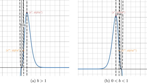The behavior of the real fixed points of the function is classified into two distinct cases: $b>1$ and $0<b<1.$ The number and nature of the fixed points of $f_{\alpha ,m}$ are described in Theorem 2.1 for the case when $b>1.$ The associated fixed points are shown in Figure 1(a). Theorem 2.3 provides a description of the number and nature of fixed points of $f_{\alpha ,m}$ for $0<b<1,$ and the associated fixed points are presented in Figure 1(b).

Figure 1. Fixed points of $f_{\alpha ,m}$ when $m(>1)$ is odd.

Theorem 2.1

(Case m is odd; $m>1$ and $b>1$). Let $f_{\alpha ,m}\in \mathcal{F}$ where m is an odd number greater than 1 and $b>1$, then there exist real numbers ${\alpha }^{*}>{\alpha }^{**}>0$ such that:

1. For $\alpha ={\alpha }^{*},f_{\alpha ,m}(x)$ has one fixed point $x^{*}.$

2. For $\alpha ={\alpha }^{**},f_{\alpha ,m}(x)$ has two fixed points $x^{**}$ and $r_3>x^{*}.$

3. For $0<\alpha <{\alpha }^{**},f_{\alpha ,m}(x)$ has two fixed points $r_1<x^{**}$ and $r_2>x^{*}.$

4. For ${\alpha }^{**}<\alpha <{\alpha }^{*},f_{\alpha ,m}(x)$ has two fixed points $x^{**}<a_1<x^{*}$ and $r_4>x^{*}.$

5. For $\alpha >{\alpha }^{*},f_{\alpha ,m}(x)$ has no fixed points.

6. For $\alpha <0,f_{\alpha ,m}(x)$ has one fixed point $r_5<0.$

Proof.

It is straightforward to show that $f_{\alpha ,m}(x)=x$ implies $\alpha =\frac{x^{m+1}}{b^x-1}.$

Let $g(x)=\frac{x^{m+1}}{b^x-1},$ g(x) satisfies the following properties:

1. g(x) is continuous.

2. g(x) has a local maximum, say ${\alpha }^{*},$ at $x^{*}.$

3. $g(x)\to -\infty$ when $x\to -\infty ,$ and $g(x)\to 0$ when $x\to \infty .$

4. g(x) is increasing on $(-\infty ,x^{*})$ and decreasing on $(x^{*},\infty ).$

To classify the nature of fixed points of $f_{\alpha ,m},$ we solve $|f{\prime }_{\alpha ,m}(x)|=1.$ Let $$p(x)=|\hspace{0.17em}\mathrm{\text{ln}}\hspace{0.17em}(b)b^x{x}^{2m+1}-m{x}^{2m}(b^x-1)|-|x^{2m}(b^x-1)|,$$ then $p(x)=0$ if and only if $|f{\prime }_{\alpha ,m}(x)|=1.$

Note that p(x) is continuous. Using Newton’s method implies that p(x) has two positive zeros $x^{*}$ and $x^{**}$ where $x^{**}<x^{*}$ and $g(x^{*})={\alpha }^{*}$ is the local maximum of $g(x).$ The sign of p(x) varies as follows:

• $p(x)>0$ for all $x\in (-\infty ,x^{**})\cup (x^{*},\infty ).$

• $p(x)<0$ for all $x\in (x^{**},x^{*}).$

• $p(x)=0$ when $x=x^{**}$ or $x=x^{*}.$

This means that:

• $f{\prime }_{\alpha ,m}(x)>1$ for all $x\in (-\infty ,x^{**})\cup (x^{*},\infty ).$

• $f{\prime }_{\alpha ,m}(x)<1$ for all $x\in (x^{**},x^{*}).$

• $f{\prime }_{\alpha ,m}(x)=1$ when $x=x^{**}$ or $x=x^{*}.$

We conclude that $x^{*}$ and $x^{**}$ are indifferent fixed points, r_i are repelling fixed points for all $i=1,2,3,\dots ,5,$ and a₁ is an attracting fixed point. □

Remark 2.2.

(Summary Table)

The following table represents the number vs. the nature of fixed points of $f_{\alpha ,m}.$

Table

α	Fixed point	#	Nature
$\alpha <0$	r5	1	Repelling
$0<\alpha <{\alpha }^{**}$	r1, r2	2	Repelling, Repelling
$\alpha ={\alpha }^{**}$	r3, $x^{**}$	2	Repelling, Indifferent
${\alpha }^{**}<\alpha <{\alpha }^{*}$	r4, a1	2	Repelling, Attracting
$\alpha ={\alpha }^{*}$	$x^{*}$	1	Indifferent
$\alpha >{\alpha }^{*}$	No fixed points

Theorem 2.3

(Case m is odd; m > 1 and $0<b<1$). Let $f_{\alpha ,m}\in \mathcal{F}$ where m is an odd number greater than 1 and $0<b<1$, then there exist real numbers ${\alpha }^{*}>{\alpha }^{**}>0$ such that

1. For $\alpha ={\alpha }^{*},f_{\alpha ,m}(x)$ has one fixed point $x^{*}.$

2. For $\alpha ={\alpha }^{**},f_{\alpha ,m}(x)$ has two fixed points $x^{**}$ and $r_3<x^{*}.$

3. For $0<\alpha <{\alpha }^{**},f_{\alpha ,m}(x)$ has two fixed points $r_1>x^{**}$ and $r_2<x^{*}.$

4. For ${\alpha }^{**}<\alpha <{\alpha }^{*},f_{\alpha ,m}(x)$ has two fixed points $x^{*}<a_1<x^{**}$ and $r_4<x^{*}.$

5. For $\alpha >{\alpha }^{*},f_{\alpha ,m}(x)$ has no fixed points.

6. For $\alpha <0,f_{\alpha ,m}(x)$ has one fixed point $r_5>0.$

Proof.

It is enough to prove that $g(x,b)=\frac{x^{m+1}}{b^x-1}$ is symmetric about the y-axis if we change b to $1/b,$ i.e., to prove that $g(x,b)=g(-x,1/b),$ where $b>0,b\ne 1.$ $$g(-x,1/b)=\frac{{(-x)}^{m+1}}{{(1/b)}^{-x}-1}.$$

Since m is odd, m + 1 is even, and thus ${(-x)}^{m+1}=x^{m+1}:$ $$g(-x,1/b)=\frac{x^{m+1}}{1/b^{-x}-1}=\frac{b^{-x}{x}^{m+1}}{1-b^{-x}}.$$

Multiplying both the numerator and denominator by b^x yields: $$g(-x,1/b)=\frac{x^{m+1}}{b^x-1}=g(x,b).$$

3. Fixed points of $f_{\alpha ,m}:$ m is even; $b>0,b\ne 1$

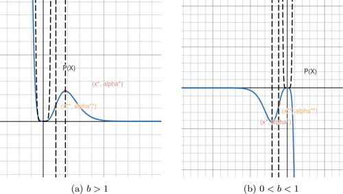
This section aims to examine the characteristics of the real fixed points of $f_{\alpha ,m}$ when m is an even number and b > 0, $b\ne 1.$ Note that the case of m = 2 is not discussed here and is left to the reader. The study focuses on two cases: b > 1 and $0<b<1.$ The nature of fixed points of $f_{\alpha ,m}$ for even m > 2 is presented in Figure 2.

Figure 2. Fixed points of $f_{\alpha ,m}$ when $m(>2)$ is even.

Theorem 3.1

(Case m is even; m > 2 and b > 1).

Let $f_{\alpha ,m}\in \mathcal{F}$ where m is an even number greater than 2 and b > 1, then there exist real numbers ${\alpha }^{*}>{\alpha }^{**}>0$ such that:

1. For $0<\alpha <{\alpha }^{**},f_{\alpha ,m}(x)$ has three fixed points $r_1<x^{**},r_2<x^{**}$, and $r_3>x^{*}.$

2. For $\alpha ={\alpha }^{**},f_{\alpha ,m}(x)$ has three fixed points $x^{**},r_4<x^{**}$, and $r_5>x^{*}.$

3. For ${\alpha }^{**}<\alpha <{\alpha }^{*},f_{\alpha ,m}(x)$ has three fixed points $x^{**}<a_1<x^{*},r_6<x^{**}$, and $r_7>x^{*}.$

4. For $\alpha ={\alpha }^{*},f_{\alpha ,m}(x)$ has two fixed points $x^{*}$ and $r_8<x^{**}.$

5. For $\alpha >{\alpha }^{*},f_{\alpha ,m}(x)$ has one fixed point $r_9<x^{**}.$

6. For $\alpha <0,f_{\alpha ,m}(x)$ has no fixed points.

Proof.

Since $f_{\alpha ,m}(x)=x$ implies $\alpha =\frac{x^{m+1}}{b^x-1}.$

Let $g(x)=\frac{x^{m+1}}{b^x-1},$ g(x) satisfies the following properties:

1. g(x) is continuous.

2. g(x) has a local maximum, say ${\alpha }^{*},$ at $x^{*}.$

3. $g(x)\to \infty$ as $x\to -\infty ,$ and $g(x)\to 0$ as $x\to \infty .$

4. g(x) is increasing on $(0,x^{*})$ and decreasing on $(-\infty ,0)\cup (x^{*},\infty ).$

To classify the nature of fixed points of $f_{\alpha ,m},$ we solve $|f{\prime }_{\alpha ,m}(x)|=1.$

Let $$p(x)=|\hspace{0.17em}\mathrm{\text{ln}}\hspace{0.17em}(b)b^x{x}^{2m+1}-m{x}^{2m}(b^x-1)|-|x^{2m}(b^x-1)|,$$ then p(x) = 0 if and only if $|f{\prime }_{\alpha ,m}(x)|=1.$

Note that p(x) is continuous. Using Newton’s method implies that p(x) has two positive zeros $x^{*}$ and $x^{**}$ where $0<x^{**}<x^{*}$ and $g(x^{*})={\alpha }^{*}$ is the local maximum of g(x). The sign of p(x) varies as follows:

• p(x) > 0 for all $x\in (-\infty ,x^{**})\cup (x^{*},\infty ).$

• p(x) < 0 for all $x\in (x^{**},x^{*}).$

• p(x) = 0 when $x=x^{**}$ or $x=x^{*}.$

This means that:

• $f{\prime }_{\alpha ,m}(x)>1$ for all $x\in (-\infty ,x^{**})\cup (x^{*},\infty ).$

• $f{\prime }_{\alpha ,m}(x)<1$ for all $x\in (x^{**},x^{*}).$

• $f{\prime }_{\alpha ,m}(x)=1$ when $x=x^{**}$ or $x=x^{*}.$

We conclude that $x^{*}$ and $x^{**}$ are indifferent fixed points, r_i are repelling fixed points for all $i=1,2,3,\dots ,9,$ and a₁ is an attracting fixed point. □

Remark 3.2.

(Summary Table)

The following table represents the number versus the nature of fixed points of $f_{\alpha ,m}.$

Table

α	Fixed point	#	Nature
$\alpha <0$	No fixed points
$0<\alpha <{\alpha }^{**}$	$r_1,r_2,r_3$	3	Repelling, repelling, repelling
$\alpha ={\alpha }^{**}$	$r_4,x^{**},r_5$	3	Repelling, indifferent, repelling
${\alpha }^{**}<\alpha <{\alpha }^{*}$	$r_6,a_1,r_7$	3	Repelling, attracting, repelling
$\alpha ={\alpha }^{*}$	$x^{*},r_8$	2	Indifferent, repelling
$\alpha >{\alpha }^{*}$	r9	1	Repelling

Theorem 3.3

(Case m is even, m > 2 and $0<b<1$).

Let $f_{\alpha ,m}\in \mathcal{F}$ where m is an even number greater than 2 and $0<b<1$, then there exist real numbers ${\alpha }^{*}<{\alpha }^{**}<0$ such that:

1. For $0>\alpha >{\alpha }^{**},f_{\alpha ,m}(x)$ has three fixed points $r_1>x^{**},r_2>x^{**}$, and $r_3<x^{*}.$

2. For $\alpha ={\alpha }^{**},f_{\alpha ,m}(x)$ has three fixed points $x^{**},r_4>x^{**}$, and $r_5<x^{*}.$

3. For ${\alpha }^{*}>\alpha >{\alpha }^{**},f_{\alpha ,m}(x)$ has three fixed points $x^{*}<a_1<x^{**},r_6>x^{**}$, and $r_7<x^{*}.$

4. For $\alpha ={\alpha }^{*},f_{\alpha ,m}(x)$ has two fixed points $x^{*}$ and $r_8>x^{**}.$

5. For $\alpha >{\alpha }^{*},f_{\alpha ,m}(x)$ has one fixed point $r_9>x^{**}.$

6. For $\alpha <0,f_{\alpha ,m}(x)$ has no fixed points.

Proof.

It is sufficient to show that $g(x,b)=\frac{x^{m+1}}{b^x-1}$ is symmetric about the origin if we replace b by $\frac{1}{b}.$ That is, to prove that $g(x,b)=-g(-x,\frac{1}{b}),$ where $b>0,b\ne 1$ and m is even.

We have $g(-x,\frac{1}{b})=\alpha =\frac{{(-x)}^{m+1}}{{(\frac{1}{b})}^{-x}-1}.$ Since m is an even number, then m + 1 is odd, and hence: $$g(-x,\frac{1}{b})=\frac{x^{m+1}}{\frac{1}{b^{-x}}-1}=-\frac{x^{m+1}{b}^{-x}}{1-b^{-x}}.$$

Multiplying the numerator and denominator by b^x, we get: $$g(-x,\frac{1}{b})=-\frac{x^{m+1}}{b^x-1}=-g(x,b).$$

4. Conclusion

This two-parameter family of functions has not been extensively studied in the literature. In this paper, we have contributed to this area by exploring the dynamics of fixed points using various techniques, including phase portraits, bifurcation diagrams, and numerical simulations. We have also derived several theorems that describe the nature and number of fixed points under different conditions of the parameters m and b. The results indicate that while the nature of fixed points remains consistent, the number of fixed points varies with changes in m and b.

Our findings have potential applications in the study of complex systems, particularly in the investigation of Julia and Fatou sets. The fractal geometry generated by the chaotic behavior of the system can provide insights into the structure and behavior of complex systems. Furthermore, our results may have practical applications in areas such as finance and engineering, where the behavior of dynamic systems is often modeled using mathematical functions. Overall, our work enhances the understanding of the dynamics of fixed points in two-parameter families of functions, which has significant implications across a broad range of disciplines.

Disclosure statement

No potential conflict of interest was reported by the author(s).

Data availability statement

The data is available upon your request.

References

- Iman, A. H., Jamil, Z. Z., & Hamada, N. H. (2022). On the dynamics of one-parameter family of functions fk(x)=kcsc(x). Iraqi Journal of Science, 63(2), 729–739.
- Kapoor, G. P., & Prasad, M. G. P. (1998). Dynamics of (ez−1)/z: The Julia set and bifurcation. Ergodic Theory and Dynamical Systems, 18(6), 1363–1383. doi:10.1017/S0143385798118011
- Nayak, T., & Prasad, M. (2014). Julia sets of Joukowski-exponential maps. Complex Analysis and Operator Theory, 8(5), 1061–1076. doi:10.1007/s11785-013-0335-1
- Sajid, M. (2016). Real fixed points and dynamics of one-parameter family of functions (bx−1)/x. Journal of the Association of Arab Universities for Basic and Applied Sciences, 21(1), 92–95. doi:10.1016/j.jaubas.2015.10.001
- Sajid, M. (2019). Chaotic behavior in real dynamics and singular values of family of generalized generating functions of Apostol Genocchi numbers. Journal of Mathematics and Computer Science, 19(01), 41–50. doi:10.22436/jmcs.019.01.06
- Sajid, M., & Alsuwaiyan, A. S. (2014). Chaotic behavior in the real dynamics of a one-parameter family of functions. International Journal of Applied Science and Engineering, 12(4), 289–301.
- Tarun Kumar, C., Nayak, T., & Senapati, K. (2018). Iteration of certain exponential-like meromorphic functions. Proceedings-Mathematical Sciences, 128(5), 1–18.