Mapping ecosystem services bundles in a heterogeneous mountain region

ABSTRACT

Recent institutional and policy frameworks prescribe the incorporation of ecosystem services (ES) into land use management and planning, favouring co-production of ES assessments by stakeholders, land planners and scientists. Incorporating ES into land management and planning requires models to map and analyze ES. Also, because ES do not vary independently, many operational issues ultimately relate to the mitigation of ES trade-offs, so that multiple ES and their interactions need to be considered. Using a highly accurate LULC database for the Grenoble urban region (French Alps), we mapped twelve ES using a range of models of varied complexity. A specific, fine-grained (less than 1 ha) LULC database at regional scale (4450 km²) added great spatial precision in individual ES models, in spite of limits of the typological resolution for forests and semi-natural areas. We analysed ES bundles within three different socio-ecosystems and associated landscape types (periurban, rural and forest areas). Such type-specific bundles highlighted distinctive ES trade-offs and synergies for each landscape. Advanced approaches combining remote sensing, targeted field data collection and expert knowledge from scientists and stakeholders are expected to provide the significant progress that is now required to support the reduction of trade-offs and enhance synergies between management objectives.

EDITED BY:

• Maria Jose Martinez-Harms

KEYWORDS:

• Ecosystem service mapping
• ecosystem service bundles
• land use and land cover
• mountain landscapes

1. Introduction

Since the Millennium Ecosystem Assessment (MEA 2005), and the formulation of the Aichi Biodiversity Targets for conservation and restoration of biodiversity and ecosystem services by 2020 (CBD 2010), ecosystem services (ES) have become mainstreamed into policy and practice. Building on this political status and on scientific progress, the ES concept has been largely disseminated, and is becoming integrated into regional to local political decisions. At the European scale, a practical implementation of ES concepts and related strategies has been targeted through the Water Framework Directive (2000) or the Biodiversity Strategy to 2020. In France, the most recent Law for Biodiversity and Landscapes (2016) explicitly incorporates ES into impact assessment and obligations for offsetting. The Ministry for Ecology has implemented a national evaluation framework for ecosystems and ES aiming to integrate ES into national and local decision processes (EFESE 2013). This initiative includes an explicit focus on methods of biophysical and economic evaluation to support public decisions, and in particular land planning. The objective is to improve the way natural capital is accounted for in the economy and in development projects.

Such a context strongly favours operational research initiatives on ES, aiming at developing co-production between stakeholders and land planners on the one hand, and the required scientific expertise on the other, for ES to be efficiently integrated in land management and planning (de Groot et al. 2010; Bierry et al. 2015; Klein et al. 2015). However, there are no standard methods through which ES may be accounted for in environmental management (Maes et al. 2016; Burkhard and Maes 2017). In practice, expert scientific knowledge is mobilized on a case by case basis, as for example in national ecosystem assessments (Schröter et al. 2016). ES indicators for a given area may be used to assess specific benefits of nature to society (Maes et al. 2016), or combined to address ecological conditions (Burkhard et al. 2012; Egoh et al. 2012; Crossman et al. 2013). Recent studies of ES bundles, defined as repeatable positive (synergies) and negative (trade-offs) ES associations in space and time (Raudsepp-Hearne et al. 2010), have confirmed the value of such analyses for supporting environmental management and land planning based on ecological understanding (Schirpke et al. 2013; Cowell and Lennon 2014; Crouzat et al. 2015; Opdam et al. 2015; Queiroz et al. 2015; Meacham et al. 2016; Baró et al. 2017; Spake et al. 2017). In particular such analyses have highlighted heterogeneity in ES bundles across adjacent municipalities or regions, along with the role of decision-makers either in maintaining particular ES bundles or in inducing a shift towards desired ES bundles to match their management strategy (see also Locatelli et al. 2017). These analyses also emphasise the interlinked character of ES, as intervening on one ES (e.g., provisioning or cultural ES) impacts the supply and use of other ES (e.g., regulating ES), changing the expression of the whole ES bundle. Overall, ES bundle analyses tackle the complexity of multifunctional landscapes while facilitating the dialogue among the diversity of associated beneficiaries (Haida et al. 2016).

At local scales, incorporating ES in land management and planning requires spatially explicit data for mapping ES (de Groot et al. 2010; Maes et al. 2012). Most ES models use Land Use and Land Cover (LULC) maps as primary proxy data (Verhagen et al. 2016; Lavorel et al. 2017). Nowadays, several LULC maps are publicly available due to growing interests in spatially explicit data in numerous fields. Among available LULC maps, Globcover data (worldwide), Corine Land Cover (Europe) and the recently produced Land Cover CES in France (©CESBIO-Theia, Inglada et al. 2017) are used most commonly. However such publicly available LULC maps are always produced at large spatial scale and despite their common use at local scales, their limited spatial resolution, typology and accuracy induce large uncertainties in ES mapping (Eigenbrod et al. 2010). High resolution maps may also be available at local scales, but are usually restricted to a single type of LULC. For instance, in Europe the Urban Atlas is available for dense urban areas, and in France the Registre Parcellaire Graphique (hereafter RPG) is based on declarations of agricultural use by farmers to claim European agricultural subsidies. However, the specific typological information available in these databases makes their direct use for ES mapping impossible; furthermore the various objects represented in such bases are not congruent across databases (different scales, different resolutions etc.), and their mapped areas are not necessarily contiguous or spatially exhaustive. Their use is therefore only possible in conjunction with other data sources in order to constitute a continuous and exhaustive LULC map at landscape or regional scale (Vannier 2011; Hubert-Moy et al. 2012; Mathian and Sanders 2014). On the other hand, remote sensing is frequently used to produce LULC data meeting needs for local-scale mapping in terms of configuration and dynamics (Hansen and Loveland 2012; Giri et al. 2013; Kuenzer et al. 2014). The best practice is therefore to merge all available databases (public and remote sensing-based) to produce a LULC map achieving sufficient precision both in terms of resolution and typology, in order to best capture local specificities.

Merging heterogeneous data for mapping ES is thus necessary and can produce great contributions to a better spatial understanding of ES patterns (Cord et al. 2017). But such an exercise may raise questions about the adequacy between available data at the desired scale and the complexity of local ecological or social processes that ES maps aim to capture (Spake et al. 2017). Studies often characterize the areas associated to each ES bundle according to their dominant LULC. For instance, ES bundles are described as linking to ‘mosaic cropland – livestock’ areas, ‘forest and towns’ or ‘urban’ areas, among others (Queiroz et al. 2015, see also Turner et al. 2014). In Crouzat et al. (2015) significant overlaps between ES bundles and land cover types were used to describe the landscapes associated to ES bundle across the French Alps. At the European scale, a recent ES assessment identified three typical bundles strongly driven by main LULC classes (Mouchet et al. 2017). Thus, existing studies often reveal ES bundles associated with first-level LULC typology (e.g. urban, periurban, agricultural, forest, and water bodies). However, at local scale there is strong evidence for variations in individual ES and in ES bundles within broad landscape types and main LULC classes, especially depending on management (Lavorel et al. 2011; Lafond et al. 2017). In terms of land planning and land management, understanding these variations is critical to go further than simplistic considerations related to spatial allocation of main land cover classes. Understanding ES associations beyond broad LULC classes thus stands out as an underachieved challenge and requires considering relevant landscape specificities for capturing more relevant ES bundles such as semi-natural linear elements (van der Zanden et al. 2013) or detailed crop sequences (2018).

This study combined three original aspects. First, we developed an intensive participatory process over more than 3 years to define, prioritize and quantify ES, aiming to address stakeholders’ needs for managing landscapes in the Grenoble area through the assessment of ES bundles (Bierry and Lavorel 2016). Second, based on these needs and on stakeholders’ local knowledge, and given known limitations of broad scale bundle analyses (Spake et al. 2017), we analysed ES bundles within characteristic landscape types associated with contrasted socio-ecosystems of the region. Third, an unusually large set of 12 ES were modelled and analysed using stakeholders and scientists’ expert knowledge, skills and data. To implement this original analysis of ES bundles, we: 1- used a very high resolution LULC database especially developed for ES modelling in the Grenoble region (French Alps); 2- analysed the relations between the LULC maps and ES bundles within characteristic landscape types; 3- we concluded by identifying contributions and limits of this approach to propose targeted areas of progress for future studies.

2. Material and methods

2.1. Landscapes of the Grenoble study area

The Grenoble employment catchment area extends over 4,450 km², for a total population of nearly 800,000 and 500,000 jobs in 2012. This largely corresponds to our study area, defined from the extent of the economic influence of the Grenoble metropolitan area (Figure 1). From the economic point of view, the limits are defined by the land plans for the Grenoble metropolitan area (Schéma de Cohérence Territoriale; SCoT¹) and neighbouring mountain areas (public inter-municipality cooperation establishments – EPCIs).

Figure 1. The Grenoble employment catchment area: location, physical geography and administrative boundaries.

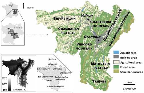
The Grenoble area is characterized by a variety of physical and natural features defining the remarkable diversity of its landscapes. The flat valley of Grésivaudan favours the Grenoble urban sprawl, a process also present in the Bièvre plain district. Three mountain ranges shape the area (Vercors, Chartreuse and Belledonne), with natural and semi-natural landscapes benefitting from numerous protection measures (Natural Regional Park, conservation areas etc.).

Overall, the Grenoble employment catchment area includes 311 municipalities within a 50 km radius, structured in ten EPCI: Grenoble metropolitan area, South Grenoble, Grésivaudan and Voiron urban area (which together constitute the Grenoble ‘Y’, thus called due to its shape on a map), Chartreuse, Vercors (the two mountain ranges outside the SCoT perimeter), Trièves, Matheysine South Grésivaudan, Bièvre-Valloire (plains and plateaus dominated by agriculture).

2.2. LULC database

Vannier et al. (2016) and Lefebvre (2014) have described in detail the data sources and methods used to build our LULC database (Table 1, levels 1, 2, 3). In short, we assembled, trimmed and cleaned the public databases from IGN² ‘BD Topo’, Urban Atlas and RPG, and pre-processed and projected RapidEye and MODIS remote sensing data on the geometry of IGN ‘BD Ortho’. These data sets were merged, segmented and then photo-interpreted to correct typological errors and complete uncharted areas in public databases. We thus produced a spatially accurate database, with a typology adapted to local needs (Table S1). An independent photo-interpreter validated the resulting maps.

Table 1. First column: Panel of selected ES; second column: indicator used to quantify the related ES; third column: model type according to Lavorel et al. (2017); fourth column: environment for ES bundle analysis (P: periurban bundle; F: forest bundle; R: and mountain rural bundle).

Ecosystem Services		Indicator	Model Type	Landscape types
				P	R	F
Biodiversity	Fauna	Vertebrate species richness, expressed in number of species/km^2.	Macro-ecological	x	x	x
	Flora	Plant species richness, expressed in number of species/km^2.	Macro-ecological	x	x	x
Provisioning	Crop production	Crop energy yield (average over 5 years, expressed as Giga Joules/Ha).	Proxy-based	x	x	.
	Forage production	Forage energy yield (average over 5 years, expressed as Giga Joules/Ha).	Proxy-based	x	x	.
	Wood production	Estimated wood production in m3/ha/year (volume of wood cut at 7cm).	Proxy-based	x	x	x
Cultural	Recreation	Outdoor recreation practice opportunities, expressed by a recreational opportunity index	Phenomenological	x	x	x
Regulation	Carbon stock	Amount of carbon stocked in above-ground and below-ground biomass as well as in dead organic matter and soils (expressed in tC/km^2).	Proxy-based	.	.	x
	Erosion	Contribution of the ecosystem to erosion risk mitigation, estimated by a non-dimensional discrete index [0;4].	Phenomenological	x	x	x
	Infiltration	Ecosystem ability to regulate water flows, expressed by a total annual infiltration indicator expressed in relative values.	Process-based	x	x	x
	Rockfall protection	Ability of forest to reduce rock fall risk on target areas, expressed by presence/absence of rockfall protection forest.	Process-based	.	.	x
	Water quality	Nitrogen retention capacity by agricultural fields, expressed in t N/ha/yr).	Process-based	x	x	.
	Pollination	Combination of demand and potential supply of pollination for agriculture, qualitative index.	Phenomenological	x	x	.

In order to further refine the description of agricultural land use (Table 1, level 4), we used medium resolution remote sensing data from MODIS (Moderate Resolution Imaging Spectroradiometer). Classification and validation methods are described in Lasseur et al. (2018). In short, we classified images based on the phenological properties of the different crop types and using altitudinal and climate information. This allowed us to produce a map of the major crop types (winter, spring or grassland) at an annual time step between 2008 and 2012. Aggregated over 5 years, these maps supported the identification of prevalent crop successions in the study area. These maps were validated with RPG data, producing an overall accuracy index (kappa index) varying between 0.78 and 0.82 depending on the year. This crop succession map was integrated into our overall LULC map.

The resulting database has a 10 meters spatial resolution over a 4450 km² extent, with a minimal object size of 0.01 ha, i.e., 100 m², and a positional accuracy of 5 to 10 meters. The typology of this database includes 34 classes of land use/land cover (Supplementary material S1), nested into four levels of precision. These encompass built-up areas (residential and commercial/industrial areas are distinguished, as well as road and railway networks, etc.), agricultural lands (specifying crop successions, grasslands, garden marketing plots or orchards). Forested and semi-natural areas are described by stands. The level of description of this typology is more detailed than what is available in most public databases, which corresponds to levels 2–3 of our typology, depending on land-use type (level 1).

2.3. ES models

A collaborative, participatory process involving local stakeholders, land managers and researchers working on the study area was used to select a panel of ES relevant to major landscape management and planning issues (Bierry and Lavorel 2016) (Table 1). First the study area was divided into three characteristic socio-ecosystems and associated landscape types within which ES bundles was then analysed. Then relevant ES were selected within each landscape type for spatial analysis.

2.3.1. Main landscape types

Analysing available ES maps of all the French Alps (Crouzat et al. 2015; Lavorel et al. 2016) (Supplementary material S2) at the scale of the Grenoble study area provides a characterization in terms of ES of the landscapes and land uses that are typical of the area (mountains vs. plains, urban sprawl in valleys vs. forested areas in mountain ranges, flatland vs. mountain agriculture – Figure 1). Piedmonts and valleys dominated by agriculture (36% of the area) support food production and provide habitat for predator species essential for biocontrol, and for plant and vertebrate species with high heritage value. Mosaic landscapes comprising multifunctional forests, grasslands and other open habitats characteristic of the northern French Alps (46% of the area) supply farming and forest products, and support multiple regulation services including pollination, carbon sequestration or water quality regulation; they also support cultural services like tourism or protected vertebrate species. At the highest altitudes cultural services dominate, including outdoor recreation, tourism and hunting, along with habitat for plant and vertebrate species of high heritage value (2% of the area). A small area (10% of the area) of semi-natural areas and forests typical of the southern French Alps and of limestone plateau rims are hotspots for the supply of regulation services like carbon sequestration and erosion control, as well as for tourism. Finally, specific forests located in areas of geological or geomorphological risks (6% of the area) protect infrastructure and houses from e.g. rockfalls).

However, to go beyond what may appear as trivial results and produce a more subtle analysis of the ecological processes of the study area, the stakeholders involved in our initiative suggested refining the analysis by focusing on three landscape types of interest, based on their knowledge, experience and on management and planning priorities: periurban areas, forested areas and rural areas in mountain regions. These were delimited geographically in the following way:

• Periurban areas were characterized by a continuous or semi-continuous residential area up to a distance of 500 m, below an altitude of 500 m a.s.l. (the main urban areas of Grenoble and Voiron are not included in this geographical definition);

• Forested areas were identified as continuously wooded tracts with a total area exceeding 400 ha;

• Rural mountain landscapes encompassed open (i.e. non-forested) areas above 500 m a.s.l.

We then analysed ES bundles specific to each of these three landscape types, considering only ES relevant to each landscape (periurban, forest, mountain rural) (Table 2).

2.3.2. ES modelling

The choice of the overall ES panel developed for this study resulted from a co-constructed selection based on (i) the interest for the local stakeholders and relevance to management issues, (ii) researchers available modelling expertise and resources, and (iii) data availability for model implementation.

Briefly, forests managers target multifunctionality, where i) profitable wood production is expected to rely on regulation services (e.g. climate regulation, erosion control) while ii) benefiting recreation and tourism, flood and water quality regulation and iii) being compatible with biodiversity protection. Planning and management for periurban areas focus on the balance between production agriculture and its supporting services, multiple ES supplied by alluvial forests and on flood regulation and cultural services demanded by the urban population (landscape aesthetic value, recreation and protected plant and vertebrate species). In mountain rural areas, priorities consider the management of the landscape mosaic shaped by livestock and wood production. These provisioning services are sustained by regulating services (erosion control, regulation of water quality and quantity) and their production supports highly valued cultural services (landscape aesthetic value, recreation) and intrinsic biodiversity values (protected plant and vertebrate species) (Lavorel et al. 2016).

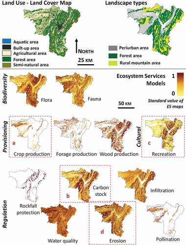
A total of 12 ES was selected (Table 1): two biodiversity indices (fauna, flora), three provisioning services (crop production, forage production, wood production), one cultural service (recreation), and six regulation services (carbon stock, erosion, infiltration, rockfall protection, water quality, pollination). The prominence of regulation services reflected the project’s focus on sustainability of ES supply (Lavorel et al. 2016). Biodiversity is viewed as both the foundation for and a direct contributor to all ES (MEA 2005).

We selected relevant modelling methods based on the classification of broad ES model types depending on relevant scales, available knowledge, expertise and data requirements, as well as the level of detail in ecological process specification (Lavorel et al. 2017). Due to lack of data and incomplete knowledge of the functional basis of some ES at the scale of operation (i.e. between the regional and landscape scale, see Figure 2), we used a significant fraction of proxy models (simple model based on expert knowledge and statistical association) or phenomenological models (which also explicitly incorporate landscape configuration and spatial processes) (Lavorel et al. 2017), mostly based on LULC maps as input data (Table 1). Table 1 presents the indicators modelled for each of the 12 ES, and Supplementary material 3 presents a full description of model choices, methods and model limits, including source data used. Most models were adapted from existing models to account for specificities of our study area landscape. Nine out of the twelve ES modelled use the dedicated LULC map produced for the study area as their most important input: fauna, agricultural production, fodder production, wood production, recreation, carbon stock, water infiltration, water quality and pollination. The most detailed typology level (level 4 – table S1) was systematically used for ES models pertaining to a single type of environment (agricultural, forest, etc.). Model limitations are also specified in (Supplementary material S3). Descriptive fact sheets provided this information to project stakeholders and are made available to future users.

Figure 2. Map produced by the 12 ES models. Model specifications are provided in Table 1 and Suppl. Mat. S3.

2.4. ES bundles analysis

ES bundle analysis had several objectives: 1- to produce an inductive, spatially-explicit classification of ES within each of the three landscape types; 2- to identify specific bundle-providing LULC classes by analysing relations between such a classification and the LULC map.

ES bundle analysis consists in identifying ES associations within a given area (Raudsepp-Hearne et al. 2010), thus partitioning the study area into internally-consistent spatial units in terms of ES supply (Spake et al. 2017). Such analysis aims to highlight similar areas in terms of ES levels (weak/high values for the same ES), and ES most distinctive of each spatial unit. After normalizing ES maps (following Paracchini et al. 2011), we performed an unsupervised classification using the ArcGis software (IsoCluster tool, ESRI Inc, Redlands, CA, USA). We then determined the number of classes through a trial and error method (within a range from 3 to 5), that was suited to local stakeholder purposes. Each of the three landscape types was independently analysed this way.

Finally, a simple Spearman’s correlation between the interpreted classes of each bundle and the LULC map was computed to assess the relevance of intensive ES modelling vs. land use prioritization based on LULC alone.

3. Results

3.1. ES maps

Given that the LULC map was used as a basis of nine out of the twelve ES modelled, and that seven out of the twelve ES models were proxy-based or phenomenological, it seems essential to first briefly describe the ES maps in relation to the information already provided by the LUCC database. Figure 2 presents the twelve ES maps produced. The complementarities of the different landscape types units of the study area are apparent from a perusal of these maps: mountain or plain areas are clearly distinctive when individual ES are considered, while each area produces one or more ES. As expected, ES spatial patterns are quite correlated with LULC spatial patterns. This results from: 1- a given LULC type being either favourable or not to a given ES, and 2- the LULC map being a predominant input in the considered ES model.

The number and level of complexity of additional variables and ecological processes incorporated into models (Table 1) define the similarity between ES spatial patterns and LULC. To illustrate this point, Figure 2 highlights maps produced by two proxy-based (agricultural production, carbon stock) and two phenomenological (recreation, erosion) models. These models exemplify the effect of the use of a gradually more complex input data: direct use of the LULC map (agricultural production, Figure 2(a)), combination of this map with one (carbon stock, Figure 2(b)) or several (recreation, Figure 2(c)) other data layers, or primary use of physical factors with LULC playing only a secondary role (erosion, Figure 2(d)):

• The agricultural production map (Figure 2(a)) displays high values in the major agricultural areas (Bièvre plain, Grésivaudan valley) and low values on hillsides, as grassland and pastures replace intensive cropping with increasing elevation. This strong dependency of the agricultural production model on agricultural land use is inherent to the model type (simple proxy). However, as we used a map of crop types at agricultural plot level, this modelling approach identifies LULC and crop successions most/least relevant to an effective ES supply.

• The carbon stock map (Figure 2(b)) also highlights contrasts predominantly defined by the LULC type given the order of magnitude of difference in stocks between forests (190 to 209 tC/km² – although variable across stand types) and agriculture and grassland areas (72 to 85 tC/km²).

• The spatial patterns of the recreation map (Figure 2(c)) are largely independent of LULC, although the LULC map is used in this model to identify the location of landscape preferences for outdoor activities. However, the map is predominantly influenced by recreation practices and accessibility, which play a fundamental role in the landscape capacity to provide the recreation ES (Byczek et al. 2018).

• The erosion model map (Figure 2(d)) relies on a phenomenological approach and also makes use of the LULC map. However, the resulting spatial patterns do not match LULC classes as the RUSLE model (Revised Universal Soil Loss Equation, ©United State Department of Agriculture) is largely determined by physical characteristics such as rainfall, soil type and slope. LULC types only modulate these primary determinants.

Thus, although most of our ES models use LULC information as input, output ES maps are not necessarily uniquely determined from this and depend more essentially on the level of complexity of the ecological processes incorporated in models. Even for the most basic models, the modelling process allows users to identify service-providing areas for a given ES (Syrbe and Walz 2012).

3.2. Landscape specific ES bundles

The three broad landscape types characterizing the study area (periurban, forest and mountain rural) occupy roughly similar surface across the study area. Periurban landscapes occupy 1194 km² (27%) and cover both periurban areas in plains and valley bottoms dominated by agriculture. Forest landscapes extend 1865 km² (42%), mostly in mountain ranges and plateaus (Vercors, Chartreuse, Belledonne, Chambarans plateau and Trièves/Matheysine). Mountain rural landscapes represent 1144 km² (25.7%) and include all upland agricultural tracts such as cropped areas in the Trièves and Matheysine plateaus, as well as grassland-dominated areas in Vercors, Belledonne, Chambarans and North Voiron.

We applied an unsupervised ES bundle classification, first for the whole region using the 12 ES, and second for each landscape type using their 8 to 10 relevant ES (Table 1). The unsupervised ES classification of the whole region retained five bundles which best captured its environmental and ES diversity. In contrast, the classification of the periurban and mountain rural landscape types retained four bundles. However, for the forest landscape type, the classification did not capture any other information than the three main forest types given by the forest LULC typology (i.e. hardwood, coniferous, mixed forests; see Suppl. Mat. S1). In this case, the typological weakness combined with the weakness of our model parameterization (Suppl. Mat. S3) prevented any further meaningful bundle analysis.

Figure 3 presents ES bundle outputs for the whole region, periurban and mountain rural landscape types, with for each area a bundle classification map, the interpretation of bundles in terms of LULC classes and the contribution of individual ES to the statistic definition of bundles (shown as mean deviation histograms). Results of the bundle analysis for the whole landscape and per landscape type aim to link ES with land cover characteristics.

Figure 3. ES bundle analysis for the whole region (top), the periurban (middle) and mountain rural (bottom) landscape types: bundle maps and contribution of individual ES to the statistic definition of classes shown as mean deviation histograms (where Fauna = Fauna, Flora = Flora, Crop = Crop production, Forage = Forage Production, Wood = Wood production, Recre = Recreation, Eros = Erosion, Infilt = Infiltration, WQual = Water Quality, Pollin = Pollination).

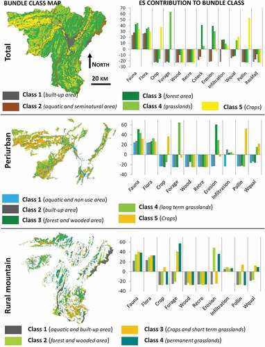
For the whole region analysis, five classes were retained. These five ES bundle classes were strongly correlated with LULC classes at level 1–2 (see S1) (r² = 0.87). The five ES bundles could then be characterised as follows (Figure 3): built-up areas with low values for all ES; semi-natural and aquatic areas with a positive value for the ability to modulate water flows (infiltration service); forest areas with high values for fauna and flora and the highest values for carbon stock, erosion and infiltration; and two classes of agricultural areas, one dominated by grasslands with the highest values for fauna and flora, forage production and high values for most regulating services (carbon stock, erosion, infiltration, water quality), and the other dominated by crops with high levels for crop production and pollination.

In the periurban landscape type, the four ES bundle classes were congruent with LULC classes at the finest typological level (level 4, see S1) (r² = 0.88). In agricultural lands, crop successions appeared essential to explain the bundle classification. The following four bundles were identified (Figure 3): two classes of crop succession depending on their intensity, one dominated by winter and spring crops without grassland, with the highest level of crop production and a high level for pollination; and the other made up of inter-annually variable crops (winter and spring annual crops, as well as fodder crops) with a high to medium level of crop and forage production, and the highest level of pollination and water quality regulation; the third class was mostly made up of permanent grasslands and wooded areas, and was the most favourable habitat for fauna and flora, and the highest levels for forage production and erosion control; finally built-up and aquatic areas had low or the lowest values for all ES.

In the mountain rural landscape type, the four ES bundles were congruent with LULC classes at the finest typological level (level 4, see S1) (r² = 0.9). Here bundles (Figure 3) highlighted the role of perennial vegetation like permanent grasslands and forests for ES supply. The following four bundles were identified: (1) areas dominated by agriculture with a high level of multifunctionality (i.e. the simultaneous supply of multiple ES) supported highest levels for fauna and flora habitats, as well as for crop and fodder production, pollination and water quality regulation; (2) woodlands and forest with the highest levels for erosion control and water infiltration; (4) permanent grasslands logically had the highest fodder production, along with rather high erosion control and infiltration and water quality regulation, and high levels for fauna and flora habitats;(5) bare and built-up areas, with the lowest levels for all ES.

5. Discussion

The results of our analysis of ES bundles within periurban and mountain rural landscapes respectively, rather than working on the entire region, highlight two strengths. First, such an analysis supports an appraisal of the region from an ES perspective that goes beyond identifying basic ES bundles associated with level 1 LULC classes (built-up, forest, agricultural, water…). Rather, it enables a finer identification of specific ES associated with given LULC types within each of these landscapes. Second, and even though the main LULC categories appear to dominate the interpretation of ES bundles, the hierarchical analysis within landscape types of significance for regional management and planning allowed us to assess the role of LULC or its inter-annual variability (in the case of agricultural land) in determining ES bundles, and thereby the potential role of management. Given the relevance of ES assessment for planning and policy (Haase et al. 2012; Queiroz et al. 2015; Locatelli et al. 2017), and for addressing sustainability issues, analyses such as this one can strongly motivate stakeholder participation. In our study, the process of ES mapping was conducted through a participatory approach with managers and planners. They suggested analysing ES bundles within landscape types was, but once bundles were identified within each landscape type they often preferred to return to individual ES they felt more familiar with (Brunet et al. 2018).

However, this work also revealed a number of limitations discussed below: 1- the simplicity of the models developed/used (mostly proxy or phenomenological models) resulting from the large extent, the regional diversity of landscapes, data availability, available knowledge and expertise; 2- the limiting typology for forest areas which takes into account only the broad stand types, whereas structure and management that play a key role in the ES supply in mountain regions would be required in a more relevant, detailed typology.

5.1. ES bundle analysis at different socio-ecosystem scales

Our analyses within the three dominant landscape types of the region were congruent with the frequent finding by ES bundle analysis at regional scale. Indeed, ES bundles essentially capture ES distribution across main LULC and landscape elements: built-up areas, aquatic and semi-natural areas, forest, grasslands (here mainly located on hills), mountain slopes and summits, and crops mainly located in plains. Such bundles are in particular congruent with studies for other European mountain region (Vigl et al. 2016, 2017). Although our results are quite similar to the regional analysis by Crouzat et al. (2015) (see 2.3.1. Main landscape types) which characterised ES bundles for the main landscape types across the entire French Alps, the within-landscape type analysis additionally highlighted the importance of distinguishing agricultural land management intensity, contrasting crop-dominated or grassland-dominated areas depending on slope and altitude. At a landscape to a regional scale, our results thus supported the consideration of major land use specificities in the LULC map construction, here differentiating crops and grasslands, and their sequencing within cultural rotations. This is not always possible when using an existing LULC database, especially when developed for a European or a national scale.

By zooming within landscape types, the contribution provided by the use of a very precise LULC database is even more important. The within-landscape types analysis highlighted the role of LULC time sequences in agricultural areas, where in the periurban landscape, crops and grassland sequences have a major role in ES supply, whereas in the mountain rural landscape, the role of permanent vegetation (forest and grassland) play a key role in ES supplying. But this landscape type analysis showed also a main limitation regarding the forest landscape type as the LULC database is unable to provide of good information on vegetation structure (open or close forests) and on management practices whereas production forests representing 89% of the forest areas of the study site. Even if the ES models specific to forest area (Wood production, Carbon Stock, Rockfall protection) take into account spatial data (land tenure, sylvo-ecoregions, forest flux inventory, see S3), the bundle analysis did not capture more specific features than the three major forest types (hardwood, coniferous, mixed forest).

However, the prominence of LULC input maps in our models strongly constrained the identification of spatial patterns of ES bundles for the periurban and mountain rural landscapes. While the segregation of ES bundles across specific LULC within each landscape type definitely reflects real contrasts in ES that were validated by stakeholders during the project final workshop, our analysis could be considered as a first tier to be compared with subsequent, refined analyses. Accounting for detailed ecological composition (e.g. for forests or for secondary successional vegetation incorporated into the semi-natural LULC class) and management practices (e.g. within forests) would enable a better LULC description or the use of more detailed biophysical variables to improve spatial/typological resolution for some ES maps, while using the same ES models. In order to target possible improvements, it appears important to analyse the constraints and limitations of the ES models developed in this study.

5.2. Modelling ES at the landscape to the regional scale

The ES modelling process was the result of co-constructed choices for ES and model selection, guided by: 1- our knowledge of the study area (field measurements and previous studies, empirical knowledge from local stakeholders and the scientific team); 2- data availability for model parameterization; and 3 – the extent of the study area (small region), along with a fine-scale resolution.

Producing a specific LULC database at a precise grain (less than 1ha) and at the scale of a small region (4450 km²) required a huge effort but added a considerable spatial information for modelling ES compared to other studies of the same type (Haase et al. 2012; Crouzat et al. 2015; Queiroz et al. 2015). As in most other ES mapping studies, LULC data is the most important ES model input (Seppelt et al. 2011; Egoh et al. 2012; Martínez-Harms and Balvanera 2012; Lautenbach et al. 2015; Verhagen et al. 2016); the association of the scale, grain and typology therefore critically controls quality of ES modelling and analysis. The typological richness along with the use of LULC classes consistent with ecological processes and a specific typology for each model partly made up for the relative simplicity of most selected models (Table 1) and of their parameterisation. For instance, whilst we used a relatively simple pollination model (Schulp et al. 2014b), the very fine spatial grain and LULC typological resolution afforded great precision for potential pollination supply. Likewise they considerably increased precision in modelling habitat of vertebrate species (Byczek 2017). Moreover, by coupling multiple input data in ES models we were able to indirectly capture important underlying processes and reduce spatial uncertainty in ES quantification (Eigenbrod et al. 2010). This was illustrated for recreation, where our phenomenological model combined multiple LULC and derived variables. Nevertheless for some ES models, the limited availability of specific data and knowledge was a great limitation. As a case in point, the InvEST model parameterization for regulation of water quality is based on literature values for main land cover types (Cabral et al. 2016). While it is certain that specific crop successions have different nitrogen retention abilities, we were unable to take advantage of our knowledge on their types and spatial distribution due to the absence of data for that parameter.

Data and knowledge availability further limited the capability of using models with intermediate to high process resolution, i.e. Tier-2 and −3 models (Grêt-Regamey et al. 2015). In particular, models used for infiltration capacity (WaterWorld) and regulation of water quality (InVEST – NDR module) could be replaced by process-based models of intermediate complexity integrating field calibration such as SWAT – the Soil & Water Assessment Tool developed to quantify the impact of land management practices in complex watersheds (Arnold et al. 2012). Further, the assessment of carbon stocks (and sequestration) would benefit from the use of process-based dynamic vegetation models such as LPJ-GUESS (Smith et al. 2001), though sufficient down-scaled climate data is still lacking for properly accounting for sub-kilometric topography-related variations in the French Alps. Estimation of biomass – related to agricultural or forested areas – would in principle be improved by earth observation data (see 5.3 below), still to be obtained for the entire Grenoble region. Implementing process-based or trait-based ES models (Lavorel et al. 2011, 2017) requires targeted field data collection and validation. This was not an option here, considering the extent of the study area (4450 km²). However, a future focus on key areas identified by local stakeholders (Quatre-montagnes, Grésivaudan valley) would enable a refined field-based analysis of ecological processes for better process-model parameterization and validation. The use of independent quantitative spatial data both to quantify biophysical variables at the landscape scale and for each type of ES model should be favoured in the future (see 5.3 below).

5.3. Avenues for improvement of ES modelling

Recent studies have demonstrated how high resolution remote sensing data coupled with field data collection can support the identification and the quantification of a wide diversity of ecosystem states and functions (Ayanu et al. 2012; Andrew et al. 2014; Cord et al. 2017; Vihervaara et al. 2017). Results from our study along with results from these works suggest that remote sensing has the potential to supply numerous data required by ES models. In particular, our work illustrates how remote sensing can be used to produce LULC maps tailored to the needs of ES models. Compared to publicly available LULC maps, the map used in our study enables a fine description of agricultural lands but remains very coarse concerning forest and semi-natural areas (respectively four and three classes for forest and semi-natural areas, compared to 18 for agricultural lands). Due to lack of suitable data, the typology does not reflect their multiple uses and their consequences for ES supply. This limitation prevented the fine analysis of ES bundles in forested areas. However, this mapping limit was mainly driven by resource allocation related to the research project aims and the priority given to agricultural areas, rather than by technical constraints. Indeed, remote sensing data has been successfully used in past studies to describe spatial heterogeneity within forest and semi-natural areas (Eva et al. 2010; Nagendra et al. 2013; Chen et al. 2015). Better characterizing forest and semi-natural areas (density, biomass, floristic diversity….) would help better modelling fauna, flora, wood production, recreation, carbon stocks, erosion mitigation, water infiltration and rockfall protection (i.e. 8 out of the 12 ES modelled). LiDAR data is available for part of the study area’s forests, and should be extended in the future, granted required financial resources.

Beyond improvement of LULC maps, remote sensing brings numerous other opportunities to overcome the current lack of data in ES mapping. In particular, recent developments of satellite-based and drone-based sensors significantly increase the affordability of multi-temporal, hyperspectral and high resolution images as well as LiDAR data. This diversity of data opens up broad prospects to a direct mapping of ecosystem functions and services. Among most promising approaches, the scaling up of plant functional traits from field measurements to regional level (Ayanu et al. 2012; Homolová et al. 2013; Andrew et al. 2014; Abelleira Martínez et al. 2016; Pettorelli et al. 2018) would allow us to extrapolate from previous plot-scale studies (e.g. Gos et al. 2016 for grassland ES; Bartholomée et al. 2018 for forest and grassland carbon stocks) using direct remote-sensing estimations of biomass production, tree allometry, soil and plant nutrient content, soil and plant water content. While processing such data required great amount of expertise and computational infrastructure so far, the recent development of cloud based interfaces such as Google Earth Engine should boost their integration into ES mapping.

Remote sensing is therefore a powerful tool for multiple facets of ES modelling, but its use requires a good knowledge of processing tools, of vector and sensor performances used at the desired grain and analysis scales. So far, the cost of data sometimes limits its use, along with the time required to acquire and process the data.

6. Conclusion

This study illustrated the benefits from combining three original components: i- an intensive participatory process, for ii- analysing ES bundles within landscape types that make sense for land planning, by iii- using a wide range of ES and associated models. Our research process and results highlighted three important conclusions. First, analysing ES bundles allowed us to assess the role of LULC or its inter-annual variability (in the case of agricultural land) for ES supply and thereby the potential role of management. This provides relevant information for land planning and management issues raised by stakeholders. Second, in order to improve the knowledge produced by such analyses, critical areas of progress are the improvement of LULC maps and the use of biophysical variables, from combined field collection and remote sensing, for better capturing ES complexity in the models. Nevertheless, while the joint use of more sophisticated models and data would definitely improve outputs for specific ES, we expect that it would only marginally modify broad ES bundles which reflect critical contrasts across each of the three landscape types. Therefore, third refinement of models and data is principally warranted for working at landscape scale where information on land use and practices is required, rather than just on land cover. Advanced approaches combining remote sensing, targeted field data collection and expert knowledge from scientists and stakeholders are expected to provide the significant progress that is now required to support the integration of multiple ES into land planning. To effectively support such improvements in data collection and analysis for land planning, intensive participatory approaches appear essential. Here we demonstrated the added value of such an approach which will subsequently support the participatory exploration of the different ways in which trade-offs could be minimized and synergies maximized between management objectives by analysing a broad range of ES models and bundles.

Acknowledgments

This research carried out on the LTSER Platform Zone Atelier Alpes contributes to project ESNET (Ecosystem Services NETwork futures for the Grenoble region) funded by ONEMA (Office national de l’Eau et des Milieux Aquatiques) and EU FP7 project OPERAs FP7-ENV-2012-two-stage-308393.

Disclosure statement

No potential conflict of interest was reported by the authors.

Supplementary material

Supplemental data for this article can be accessed here.

Notes

1. ‘This urban planning document defines the main management and planning options of the Grenoble area for the next 20 years: environment, housing, business, public services, economic development, agriculture, transport’, http://scot-region-grenoble.org/ (SCoT Grenoble – Site Officiel 2018).

2. French National Institute in charge of all nationwide data collection and formatting for mapping purposes.

References

- Abelleira Martínez OJ, Fremier AK, Günter S, Ramos Bendaña Z, Vierling L, Galbraith SM, Bosque-Pérez NA, Ordoñez JC. 2016. Scaling up functional traits for ecosystem services with remote sensing: concepts and methods. Ecol Evol. 6:4359–4371. doi:10.1002/ece3.2201.
- Andrew ME, Wulder MA, Nelson TA. 2014. Potential contributions of remote sensing to ecosystem service assessments. Prog Phys Geog. 38(3):328–353. doi:10.1177/0309133314528942.
- Arnold JG, Moriasi DN, Gassman PW, Abbaspour KC, White M, Srinivasan R, Santhi C, Harmel D, van Griensven A, Van Liew MW, et al. 2012. SWAT: model use, calibration, and validation. Biol Syst Eng Pap Publ. 55(4): 1491–1508
- Ayanu YZ, Conrad C, Nauss T, Wegmann M, Koellner T. 2012. Quantifying and mapping ecosystem services supplies and demands: a review of remote sensing applications. Environ Sci Technol. 46(16):8529–8541. doi:10.1021/es300157u.
- Baró F, Gómez-Baggethun E, Haase D. 2017. Ecosystem service bundles along the urban-rural gradient: insights for landscape planning and management. Ecosyst Serv. 24:147–159. doi:10.1016/j.ecoser.2017.02.021.
- Bartholomée O, Grigulis K, Colace MP, Arnoldi C, Lavorel S. 2018. Methodological uncertainties in estimating carbon storage in temperate forests and grasslands. Ecol Indic. 95(1): 331–342. doi:10.1016/j.ecolind.2018.07.054.
- Bierry A, Lavorel S. 2016. Implication des parties prenantes d’un projet de territoire dans l’élaboration d’une recherche à visée opérationnelle. Sciences Eaux et Territoires. Numéro spécial Gestion intégrée des territoires et des écosystèmes : vers une meilleure compréhension des trajectoires futures de l’usage des sols et leurs conséquences pour la biodiversité et les services écosystémiques. 21: 18–23..
- Bierry A, Quétier F, Baptist F, Wegener L, Lavorel S. 2015. Apports potentiels du concept de services écosystémiques au dialogue territorial. Sceinces Eaux et Territoires online. http://www.set-revue.fr/node/http%3A//www.set-revue.fr/apports-concept-services-ecosystemiques-territoires.
- Brunet L, Tuomisaari J, Lavorel S, Crouzat E, Bierry A, Peltola T, Arpin I. 2018. Actionable knowledge for land use planning: making ecosystem services operational. Land Use Policy. 72:27–34. doi:10.1016/j.landusepol.2017.12.036.
- Burkhard B, Kroll F, Nedkov S, Müller F. 2012. Mapping ecosystem service supply, demand and budgets. Ecol Indic. Challenges of sustaining natural capital and ecosystem servicesQuantification, modelling & valuation/accounting. 21(octobre):17–29. doi:10.1016/j.ecolind.2011.06.019.
- Burkhard B, Maes J, editor. 2017. Mapping ecosystem services. Sofia (Bulgaria): Pensoft Publishers; p. 374.
- Byczek C. 2017. Une analyse multi-modèles des services écosystémiques de la région urbaine de Grenoble. Grenoble Alpes. Thesis, University
- Byczek C, Longaretti P-Y, Renaud J, Lavorel S. 2018. Benefits of crowd-sourced GPS information for modelling the recreation ecosystem service. PLoS One. 13:e0202645. doi:10.1371/journal.pone.0202645.
- Cabral P, Feger C, Levrel H, Chambolle M, Basque D. 2016. Assessing the impact of land-cover changes on ecosystem services: a first step toward integrative planning in Bordeaux, France. Ecosyst Serv. 22(Part.B):318–327. doi:10.1016/j.ecoser.2016.08.005.
- CBD (Convention on Biological Diversity). 2010. Aichi biodiversity targets of the strategic plan 2011–2020. http://www.cbd.int/sp/targets/.
- Chen Y, Lu D, Luo G, Huang J. 2015. Detection of vegetation abundance change in the alpine tree line using multitemporal landsat thematic mapper imagery. Int J Remote Sens. 36(18):4683–4701. doi:10.1080/01431161.2015.1088675.
- Cord AF, Brauman KA, Chaplin-Kramer R, Huth A, Ziv G, Seppelt R. 2017. Priorities to advance monitoring of ecosystem services using earth observation. Trends Ecol Evol. 32:416–428. doi:10.1016/j.tree.2017.03.003.
- Cowell R, Lennon M. 2014. The utilisation of environmental knowledge in land-use planning: drawing lessons for an ecosystem services approach. Environ Plann C Gov Policy. 32(2):263–282. doi:10.1068/c12289j.
- Crossman ND, Burkhard B, Nedkov S, Willemen L, Petz K, Palomo I, Drakou EG, Martín-Lopez B, McPhearson T, Boyanova K, et al. 2013. A blueprint for mapping and modelling ecosystem services. Ecosyst Serv. Special Issue on Mapping and Modelling Ecosystem Services. 4:4–14. doi:10.1016/j.ecoser.2013.02.001.
- Crouzat E, Mouchet M, Turkelboom F, Byczek C, Meersmans J, Berger F, Verkerk PJ, Lavorel S. 2015. Assessing bundles of ecosystem services from regional to landscape scale: insights from the French Alps. J Appl Ecol. 52(5):1145–1155. doi:10.1111/1365-2664.12502.
- de Groot RS, Alkemade R, Braat L, Hein L, Willemen L. 2010. Challenges in integrating the concept of ecosystem services and values in landscape planning, management and decision making. Ecol Complex. Ecosystem Services – Bridging Ecology, Economy and Social Sciences. 7(3):260–272. doi:10.1016/j.ecocom.2009.10.006.
- Egoh B, Evangelia D, Bonnet DM, Joachim M, Louise W. 2012. Indicators for mapping ecosystem services: a review. Publications Office of the European Union. http://publications.jrc.ec.europa.eu/repository/handle/111111111/26749.
- Eigenbrod F, Armsworth PR, Anderson BJ, Heinemeyer A, Gillings S, Roy DB, Thomas CD, Gaston KJ. 2010. The impact of proxy-based methods on mapping the distribution of ecosystem services. J Appl Ecol. 47(2):377–385. doi:10.1111/j.1365-2664.2010.01777.x.
- Eva H, Carboni S, Achard F, Stach N, Durieux L, Faure J-F, Mollicone D. 2010. Monitoring forest areas from continental to territorial levels using a sample of medium spatial resolution satellite imagery. ISPRS J Photogramm Remote Sens. 65:191–197. doi:10.1016/j.isprsjprs.2009.10.008.
- Giri C, Pengra B, Long J, Loveland TR. 2013. Next generation of global land cover characterization, mapping, and monitoring. Int J Appl Earth Obs Geoinf. 25(décembre):30–37. doi:10.1016/j.jag.2013.03.005.
- Gos P, Loucougaray G, Colace MP, Arnoldi C, Gaucherand S, Dumazel D, Girard L, Delorme S, Lavorel S. 2016. Relative contribution of soil, management and traits to co-variations of multiple ecosystem properties in grasslands. Oecologia. 180:1001–1013. doi:10.1007/s00442-016-3551-3.
- Grêt-Regamey A, Weibel B, Kienast F, Rabe S-E, Zulian G. 2015. A tiered approach for mapping ecosystem services. Ecosyst Serv. Best Practices for Mapping Ecosystem Services. 13:16–27. doi:10.1016/j.ecoser.2014.10.008.
- Haase D, Schwarz N, Strohbach M, Kroll F, Seppelt R. 2012. Synergies, trade-offs, and losses of ecosystem services in urban regions: an integrated multiscale framework applied to the Leipzig-Halle region. Germany Ecol Soc. 17. doi:10.5751/ES-04853-170322.
- Haida C, Rüdisser J, Tappeiner U. 2016. Ecosystem services in mountain regions: experts’ perceptions and research intensity. Reg Environ Change. 16:1989–2004. doi:10.1007/s10113-015-0759-4.
- Hansen MC, Loveland TR. 2012. A review of large area monitoring of land cover change using landsat data. Remote Sens Environ. 122(juillet):66–74. doi:10.1016/j.rse.2011.08.024.
- Homolová L, Malenovský Z, Clevers JGPW, García-Santos G, Schaepman ME. 2013. Review of optical-based remote sensing for plant trait mapping. Ecol Complex. 15(septembre):1–16. doi:10.1016/j.ecocom.2013.06.003.
- Hubert-Moy L, Nabucet J, Vannier C, Lefebvre A. 2012. Mapping ecological continuities: which data for which territorial level? Application to the forest and hedge network. Revue Internationale De Géomatique. 22(4):619–640. doi:10.3166/rig.22.619-640.
- Inglada J, Vincent A, Arias M, Tardy B, Morin D, Rodes I. 2017. Operational high resolution land cover map production at the country scale using satellite image time series. Remote Sens. 9:95. doi:10.3390/rs9010095.
- Klein TM, Celio E, Grêt-Regamey A. 2015. Ecosystem services visualization and communication: A demand analysis approach for designing information and conceptualizing decision support systems. Ecosyst Serv. Best Practices for Mapping Ecosystem Services. 13:173–83. doi:10.1016/j.ecoser.2015.02.006.
- Kuenzer C, Ottinger M, Wegmann M, Guo H, Wang C, Zhang J, Dech S, Wikelski M. 2014. Earth observation satellite sensors for biodiversity monitoring: potentials and bottlenecks. Int J Remote Sens. 35(18):6599–6647. doi:10.1080/01431161.2014.964349.
- Lafond V, Cordonnier T, Mao Z, Courbaud B. 2017. Trade-offs and synergies between ecosystem services in uneven-aged mountain forests: evidences using Pareto fronts. Eur J For Res. 136(5–6): 997–1012.
- Lasseur R, Vannier C, Lefebvre J, Longaretti P-Y, Lavorel S. 2018. Landscape scale modelling of agricultural land use for the quantification of ecosystem services. Journal of Applied Remote Sensing. 12(4), 046024 (30 November 2018). https://doi.org/10.1117/1.JRS.12.046024.
- Lautenbach S, Anne-Christine Mupepele CF, Dormann HL, Stefan Schmidt SS, Scholte K, Ralf Seppelt AJ, van Teeffelen A, Verhagen W, Volk M. 2015. Blind spots in ecosystem services research and implementation. BioRxiv. décembre. doi:10.1101/033498.
- Lavorel S, Bayer A, Bondeau A, Lautenbach S, Ruiz-Frau A, Schulp N, Seppelt R, Verburg P, van Teeffelen A, Vannier C, et al. 2017. Pathways to bridge the biophysical realism gap in ecosystem services mapping approaches. Ecol Indic. 74(mars):241–260. doi:10.1016/j.ecolind.2016.11.015.
- Lavorel S, Bierry A, Crouzat E. 2016. Gestion intégrée des territoires par une approche par les réseaux de services. Sciences Eaux et Territoires. Numéro spécial Gestion intégrée des territoires et des écosystèmes : vers une meilleure compréhension des trajectoires futures de l’usage des sols et leurs conséquences pour la biodiversité et les services écosystémiques. 21:10–17.
- Lavorel S, Grigulis K, Lamarque P, Colace M-P, Garden D, Girel J, Pellet G, Douzet R. 2011. Using plant functional traits to understand the landscape distribution of multiple ecosystem services. J Ecol. 99(1):135–147. doi:10.1111/j.1365-2745.2010.01753.x.
- Lefebvre J. 2014. Méthode, cartographies et analyses des dynamiques des modes d’occupation des sols sur le bassin d’emploi de la région grenobloise entre 1998 et 2009. Grenoble: INRIA, CNRS. Rapport d’activité.
- Locatelli B, Lavorel S, Sloan S, Tappeiner U, Geneletti D. 2017. Characteristic trajectories of ecosystem services in mountains. Front Ecol Environ. 15:150–159. doi:10.1002/fee.1470.
- Maes J, Egoh B, Willemen L, Liquete C, Vihervaara P, Schägner JP, Grizzetti B, Drakou EG, La Notte A, Zulian G, et al. 2012. Mapping ecosystem services for policy support and decision making in the European Union. Ecosyst Serv. 1(1):31–39. doi:10.1016/j.ecoser.2012.06.004.
- Maes J, Liquete C, Teller A, Erhard M, Paracchini ML, Barredo JI, Grizzetti B, Cardoso A, Somma F, Petersen J-E, et al. 2016. An indicator framework for assessing ecosystem services in support of the EU biodiversity strategy to 2020. Ecosyst Serv. 17:14–23. doi:10.1016/j.ecoser.2015.10.023.
- Martínez-Harms MJ, Balvanera P. 2012. Methods for mapping ecosystem service supply: a review. Int J Biodivers Sci Ecosyst Serv Manage. http://www.tandfonline.com/doi/abs/10.1080/21513732.2012.663792.
- Mathian H, Sanders L. 2014. Spatio-temporal approaches: geographic objects and change process. Hoboken (NJ): John Wiley & Sons, Inc. doi:10.1002/9781118649213.
- MEA. 2005. Living beyond our means - natural assets and human well-being - statement from the board. Washington DC: Millennium Ecosystem Assessment.
- Meacham M, Queiroz C, Norström AV, Peterson GD. 2016. Social-ecological drivers of multiple ecosystem services: what variables explain patterns of ecosystem services across the Norrström drainage basin? Ecol Soc. 21. doi:10.5751/ES-08077-210114.
- Mouchet MA, Paracchini ML, Schulp CJE, Stürck J, Verkerk PJ, Verburg PH, Lavorel S. 2017. Bundles of ecosystem (dis)services and multifunctionality across European landscapes. Ecol Indic. 73:23–28. doi:10.1016/j.ecolind.2016.09.026.
- Nagendra H, Lucas R, Honrado JP, Jongman RHG, Tarantino C, Adamo M, Mairota P. 2013. Remote sensing for conservation monitoring: assessing protected areas, habitat extent, habitat condition, species diversity, and threats. Ecol Indic. Biodiversity Monitoring. 33:45–59. doi:10.1016/j.ecolind.2012.09.014.
- Opdam P, Coninx I, Dewulf A, Steingröver E, Vos C, van der Wal M. 2015. Framing ecosystem services: affecting behaviour of actors in collaborative landscape planning? Land Use Policy. 46:223–231. doi:10.1016/j.landusepol.2015.02.008.
- Paracchini ML, Cesare Pacini M, Laurence MJ, Pérez-Soba M. 2011. An aggregation framework to link indicators associated with multifunctional land use to the stakeholder evaluation of policy options. Ecol Indic. Spatial information and indicators for sustainable management of natural resources. 11(1):71–80. doi:10.1016/j.ecolind.2009.04.006.
- Pettorelli N, Schulte to Bühne H, Tulloch A, Dubois G, Macinnis‐Ng C, Queirós AM, Keith DA, Wegmann M, Schrodt F, Stellmes M, et al. 2018. Satellite remote sensing of ecosystem functions: opportunities, challenges and way forward. Remote Sens Ecol Conserv. 4:71–93. doi:10.1002/rse2.59.
- Queiroz C, Meacham M, Kristina Richter AV, Norström EA, Norberg J, Peterson G. 2015. Mapping bundles of ecosystem services reveals distinct types of multifunctionality within a Swedish landscape. AMBIO. 44(1):89–101. doi:10.1007/s13280-014-0601-0.
- Raudsepp-Hearne C, Peterson GD, Bennett EM. 2010. Ecosystem service bundles for analyzing tradeoffs in Diverse landscapes. Proc Natl Acad Sci U S A. 107(11):5242–5247. doi:10.1073/pnas.0907284107.
- Schirpke U, Leitinger G, Tasser E, Schermer M, Steinbacher M, Tappeiner U. 2013. Multiple ecosystem services of a changing Alpine landscape: past, present and future. Int J Biodivers Sci Ecosyst Serv Manage. 9(2):123–135. doi:10.1080/21513732.2012.751936.
- Schröter M, Albert C, Marques A, Tobon W, Lavorel S, Maes J, Brown C, Klotz S, Bonn A. 2016. National ecosystem assessments in Europe: a review. BioScience. 66(10):813–828. doi:10.1093/biosci/biw101.
- Schulp CJE, Lautenbach S, Verburg PH. 2014. Quantifying and mapping ecosystem services: demand and supply of pollination in the European Union. Ecol Indic. 36(janvier):131–141. doi:10.1016/j.ecolind.2013.07.014.
- SCoT Grenoble - Site Officiel. 2018. Scot 2030; [accessed 2018 Oct 23]. http://scot-region-grenoble.org/.
- Seppelt R, Dormann CF, Eppink FV, Lautenbach S, Schmidt S. 2011. A quantitative review of ecosystem service studies: approaches, shortcomings and the road ahead. J Appl Ecol. 48(3):630–636. doi:10.1111/j.1365-2664.2010.01952.x.
- Smith B, Prentice IC, Sykes MT. 2001. Representation of vegetation dynamics in the modelling of terrestrial ecosystems: comparing two contrasting approaches within European climate space. Glob Ecol Biogeogr. 10:621–637. doi:10.1046/j.1466-822X.2001.t01-1-00256.x.
- Spake R, Lasseur R, Crouzat E, Bullock JM, Lavorel S, Parks KE, Schaafsma M, Bennett EM, Maes J, Mulligan M, et al. 2017. Unpacking ecosystem service bundles: towards predictive mapping of synergies and trade-offs between ecosystem services. Glob Environ Change. 47:37–50. doi:10.1016/j.gloenvcha.2017.08.004.
- Syrbe R-U, Walz U. 2012. Spatial indicators for the assessment of ecosystem services: providing, benefiting and connecting areas and landscape metrics. Ecol Indic. Challenges of sustaining natural capital and ecosystem services. 21:80–88. doi:10.1016/j.ecolind.2012.02.013.
- Turner KG, Odgaard MV, Bocher PK, Dalgaard T, Svenning JC. 2014. Bundling ecosystem services in Denmark: trade-offs and synergies in a cultural landscape. Landsc Urban Plan. 125:89–104. doi:10.1016/j.landurbplan.2014.02.007.
- van der Zanden EH, Verburg PH, Mücher CA. 2013. Modelling the spatial distribution of linear landscape elements in Europe. Ecol Indic. 27:125–136. doi:10.1016/j.ecolind.2012.12.002.
- Vannier C. 2011. Observation et modélisation spatiale de pratiques agricoles territorialisées à partir de données de télédétection : application au paysage bocager. Rennes 2. http://www.theses.fr/2011REN20046.
- Vannier C, Lefebvre J, Longaretti P-Y, Lavorel S. 2016. Patterns of landscape change in a rapidly urbanizing mountain region. EJG. octobre. doi:10.4000/cybergeo.27800.
- Verhagen W, Astrid JA, Teeffelen V, Compagnucci AB, Poggio L, Gimona A, Verburg PH. 2016. Effects of landscape configuration on mapping ecosystem service capacity: a review of evidence and a case study in Scotland. Landsc Ecol. 31(7):1457–1479. doi:10.1007/s10980-016-0345-2.
- Vigl LE, Schirpke U, Tasser E, Tappeiner U. 2016. Linking long-term landscape dynamics to the multiple interactions among ecosystem services in the European Alps. Landsc Ecol. 31:1903–1918. doi:10.1007/s10980-016-0389-3.
- Vigl LE, Tasser E, Schirpke U, Tappeiner U. 2017. Using land use/land cover trajectories to uncover ecosystem service patterns across the Alps. Reg Environ Change. 17:2237–2250. doi:10.1007/s10113-017-1132-6.
- Vihervaara P, Auvinen A-P, Mononen L, Törmä M, Ahlroth P, Anttila S, Böttcher K, Forsius M, Heino J, Heliölä J, et al. 2017. How essential biodiversity variables and remote sensing can help national biodiversity monitoring. Glob Ecol Conserv. 10:43–59. doi:10.1016/j.gecco.2017.01.007.