Combining Ecological Niche Models and ecosystem services indicators to assess impacts of climate change on kelp: application to French coasts

ABSTRACT

Kelp forests, primarily Laminaria digitata, provide a broad range of ecosystem services of high social, economic, and ecological value and are considered one of the most productive ecosystems on the planet. Several studies have shown that kelp ecosystems are regressing in response to multiple stressors, especially climate change, which could lead to local extinctions. This may induce a decrease in the ecosystem services provided. Many studies use ecological niche models (ENM) to project potential future species distributions under climate change scenarios; however, no study has projected the future supply of ecosystem services resulting from shifts in species ranges and changes in biomass. In this study, using French coasts as a case study, we developed a new and reproducible methodological framework that combines ENM and ecosystem services indicators to assess impacts of climate change on ecosystem services supplied by kelp. To this end, we first identified ecosystem services currently provided by kelp and then used ENM to project future kelp distribution from 2041 to 2050 under climate scenarios RCP2.6 and RCP8.5. Finally, by estimating the biomass of kelp, we assessed the current and future ecosystem services provided by kelp.

Edited by:

• Evangelia Drakou

KEYWORDS:

• Laminaria digitata
• climate change
• ecosystem services indicators
• ecological niche models
• projections

1. Introduction

Impacts of climate change on terrestrial and marine biodiversity have been documented extensively in the literature over the past two decades (Lenoir et al. 2020; Trisos et al. 2020). A large amount of evidence indicates that changes in climate over the next several decades will shift future species ranges towards the poles (e.g. Morley et al. 2018) and, for marine species, deeper depths (e.g. Duffy and Chown 2017), cause local extinctions (e.g. McLean et al. 2021), habitat fragmentation (e.g. Jonsson et al. 2018), species invasions, and impacts on life history traits (e.g. Byrne et al. 2020), abundances (e.g. Stuart-Smith 2021), and trophic networks (e.g. Vinagre et al. 2019).

Biodiversity loss associated to an impaired integrity of ecosystems as a consequence of climate change may have negative effects on the delivery of ecosystem services. Ecosystem services (ES) is a concept popularised by the Millennium Ecosystem Assessment (MEA 2005) and evolved to the concept of Nature’s Contributions to People (NCP) that includes a wide range of descriptions of human dependence on nature (Pascual et al. 2017). Ecosystem services and Nature’s Contributions to People refer to all the contributions that nature makes to human welfare but led to some confusion about the characteristics between ES and NCP that have been addressed in the literature (Kadykalo et al. 2019). The Intergovernmental Science-Policy Platform on Biodiversity and Ecosystem Services (IPBES) argues that healthier ecosystems provide, quantitatively and qualitatively, more ES than unhealthy ecosystems and that climate change is the first driver of ecosystem services loss (Pörtner et al. 2021).

The Ecosystem services concept was developed to support ecosystem and biodiversity conservation by providing decision-makers and stakeholders with comprehensive arguments for managing biodiversity. Understanding the services provided by an ecosystem should encourage management measures targeting the sustainability of socio-ecological systems. The IPBES recently warned again on the urgent need to understand and assess services, or Nature’s Contributions to People (NCP), and their underlying mechanisms to be able to reach Aichi Biodiversity targets (Pörtner et al. 2021).

In the marine realm, sensitive ecosystems like coastal marine vegetation that support a vast diversity of marine life and important ecosystem services, such as fisheries and carbon sequestration are at a high to very high risk of climate negative impacts (Edgar et al. 2000; Li et al. 2018; Sanderman et al. 2018). One of the most important coastal marine vegetation ecosystems are kelp forests, large brown seaweed of the Laminariales order. Kelp forests, dominating rocky reefs throughout the world’s temperate seas (Filbee-Dexter and Wernberg 2018), provide a broad range of ES of high social, economic, and ecological value (Vásquez et al. 2014; Bennett et al. 2016). Indeed, they support a high biodiversity (O’Brien and Scheibling 2016), are considered as one of the most productive ecosystems on the planet (Wernberg et al. 2019) and function as “foundation species” (Teagle et al. 2017), mitigate local environmental conditions (such as nutrient dynamics (Schmitz et al. 2010)), water flow (Arkema et al. 2013) and physical disturbance (Wernberg et al. 2013), and are a major source of organic carbon due to the shedding of old fronds, which supports a continuous flow of export material at large scales (Krause-Jensen and Duarte 2016). Kelp forests provide a wide range of essential ES (Wernberg et al. 2019): ES of direct-use benefits for human well-being (e.g. kelp harvesting for alginate extraction, providing habitats for commercial and recreational fish species, tourism; these are ES that contribute most to the high economic value of kelp (Blamey and Bolton 2018)) and of indirect-use benefits from the underpinning ecological processes (e.g. climate regulation, carbon sequestration, coastline protection, nutrient cycling; Krause-Jensen et al. 2018) or from their non-use value (e.g. scientific or cultural importance, Smale et al. 2013).

Due to the decrease in coastal ecosystem health in recent decades, the scientific literature reports widespread losses in kelp populations (Voerman et al. 2013; Araújo et al. 2016; Assis et al. 2018) as a consequence of multiple stressors, such as global warming (Krumhansl et al. 2016; Smale 2020), increase in storm frequency (Smale and Vance 2016), increase in herbivore pressure (Steneck et al. 2013), and excessive harvesting (Lorentsen et al. 2010). Loss of kelp forests at a large spatial scale will have major implications for biodiversity and human well-being (Voerman et al. 2013). This rapid loss raises global awareness, and to conserve kelp populations, several authors call for prioritising and rapidly acquiring knowledge of the processes that underlie the supply of kelp ES (Smale et al. 2013) and kelp’s response to climate change (Smale 2020). However, in the European Union, kelp forests are not specifically targeted in the Habitats Directive as a marine habitat in themselves (Teagle et al. 2017). Instead, they are considered components of “reef” habitats (Beck and Airoldi 2007), for which conservation measures are not a priority. Besides, projecting potential future loss of ES provided by kelps as a response to anthropogenic pressure, could be an efficient way to better manage this ecosystem by providing decision-makers and stakeholders with an order of magnitude of the loss of benefits for human populations.

In marine ecology, projecting future species distributions as a response to climate change using Ecological Niche Models (ENM) has become a routine (e.g. Feng et al. 2019; Melo-Merino et al. 2020). ENM use a variety of statistical methods to combine species occurrence data and spatial environmental data to predict the suitability of sites for a specific species. Future shifts in species distribution can thus be predicted under different climate-change scenarios (Thuiller et al. 2009). However, projecting potential loss or gain of ES associated to a changing spatial distribution or biomass are still rare. Combining biophysical indicators of ES and ENM could help to assess potential future supply of ES by kelp forests. Existing studies have projected future ranges of kelp forests as a response to climate change (Bekkby et al. 2009; Raybaud et al. 2013; Gregr et al. 2019) but they used old modelling frameworks relying on some misuses and proxies that are widely practiced and rarely addressed together in the ENM literature (see Ben Rais Lasram et al. 2020 for details). In this study, we propose to use a new ENM framework (Ben Rais Lasram et al. 2020) that addresses these limits in order to project future kelp spatial distribution.

ENM outputs have a spatial dimension since they consist on distribution maps (binary occurrences or probability of presence), however, ES indicators do not necessarily have a spatial dimension. Thus, only ES indicators related to spatial dimension can be projected using ENM. Moreover, many ES indicators are related to kelp biomass (for e.g. the quantity of alginate extracted, nutrient cycling) but ENM doesn’t project any biomass. Thus, there is a need to assess future kelp biomass according to their range shift and loss projected by ENM.

Besides, since the emergence of the concept of ES, much research has put the focus on the monetary value dimension (e.g. Costanza et al. 1997; Barbier et al. 2009; TEEB 2010), but recent literature revealed the limits of pure economic assessments and argued that ES and NCP should clearly not be restricted to monetary value (Gómez-Baggethun et al. 2014). This led to the concept of plural values of nature and the development of methods related to integrated valuation of ES (Dendoncker et al. 2018; Rincón-Ruiz et al. 2019). Integrated valuation of ES has become a frontier in ecosystem services science and IPBES has adopted the plural value of nature as perspective (Pörtner et al. 2021). The integrated valuation of ES requires the development of accurate and reliable ES indicators which is not an easy task given the absence of a formalized methodology and the context specificity of each ecosystem.

For kelps for example, economic valuation of ES is widely practiced (e.g. US$1,000,000 per km of coastline per year in Bennett et al. 2016) and ES have been clearly stated in various studies often related to direct-use benefits (e.g. alginate extraction) and indirect-use benefits (e.g. carbon sequestration) but indicators are not systematically proposed. This absence of quantification of ES in general and their spatial dimension related or not to biomass in particular, prevent the combination of ENM and ES indicators in order to project potential future supply in a context of climate change.

Taking northern France as a case study (the most important extraction zone in Europe along with Norway with approximately 50000 t of kelps collected each year, Davoult et al. (2011)), the aim of this paper is to propose a methodological framework combining ENM and ES indicators in order to project potential future ES supply as a response to climate change. To that aim, we first made an exhaustive inventory of ES provided by kelps based on a literature review and identified those that could be related to a spatial dimension through their occurrences or biomass. We then, when possible, developed our own quantitative and spatialized indicators for ES reported in the literature but not quantified nor spatialized. After that, we used ENM to project future kelp distribution using two Representative Concentration Pathway (RCP) scenarios (i.e. RCP2.6 and RCP8.5) and developed a proxy in order to assess future biomass since several ES indicators are related to kelp biomass (for e.g. the quantity of alginate extracted, nutrient cycling). Finally, we fed quantitative and spatialized ES indicators with future kelps occurrences or biomass in order to assess their future supply loss or gain.

To our knowledge, only a few studies have used ENM to predict or project ES provided by biodiversity (for e.g. Civantos et al. (2012) linked future spatial distribution of terrestrial vertebrates obtained from ENM to the invertebrate and rodent pests-control service they provide, and Liquete et al. (2016) linked ENM to the lifecycle maintenance service of two fish species in the Mediterranean Sea) and none of them included kelp forest ecosystems.

Our methodological framework could help to implement appropriate conservation measures by given insights into the future trends of ES supply.

2. Materials and methods

Our methodological framework is summarized in the workflow diagram (Figure 1) and consists of four main steps that are detailed later in this section.

Figure 1. Methodological framework and processing steps. Four main steps were performed: inventorying ecosystem services (ES) indicators (see section 2.2), running Ecological Niche Models (ENM) (see section 2.3); estimating biomass, and quantifying ES (see section 2.4). Rounded rectangles correspond to actions performed like preparing data or running models (only BIOMOD model is depicted by a hexagon). Pointed rectangles symbolize data and maps (used or produced).

First of all, we performed a review of the literature on kelps in order to set an exhaustive inventory of the related ES. A part of the inventoried ES is quantitative and can be assessed by indicators directly available in the literature as equations. Some of them have a spatial dimension because including explicitly the kelp distribution or because they include kelp biomass that can be related to spatial distribution. Another part of the inventoried ES hasn’t been quantified yet in the literature and we had to develop our own indicators (quantified using equations we have implemented) related to a spatial dimension. These indicators can be qualified as “projectable” because they can be quantified according to the projected future distribution or biomass resulting from ENM.

Second, we used the new ENM framework proposed by Ben Rais Lasram et al. (2020) in order to project future kelp distribution under two climate scenarios RCP2.6 and RCP8.5. ENM outputs consist on binary occurrences or probabilities of presence but some ES indicators include biomass. We thus need to translate probabilities of presence into biomass. To do that, we assigned a biomass to each class of probability of presence by overlapping the map of probability of presence of kelp obtained from ENM to two biomass maps found in the literature and reporting L. digitata biomass in two local sites considered as references in France (Morlaix and Molène archipelago). We highlight here that the relationship between species probabilities of occurrences and biomass and between biomass and the provided ES might not be linear.

Finally, we fed the “projectable” ES indicators with current and future kelps occurrences or biomass in order to assess the future trend of the supply.

2.1. Description of the kelp species and study area

2.1.1. Species presentation

The common term “kelp” is used in the broadest sense to indicate most large brown seaweed (Fraser 2012) which dominates rocky reefs throughout the world’s temperate seas (Steneck et al. 2002). We considered the order Laminariales, which many authors (Bertocci et al. 2015) consider to be the “true” (e.g. Steneck et al. 2002) and “technical” (e.g. Dayton 1985) definition of “kelp”. We focused specifically on Laminaria digitata, which belongs to the dominant kelp genus in the North Atlantic (Smale et al. 2013). L. digitata is one of the most abundant, studied, and commercially important European kelp species (Bartsch et al. 2008).

Global distribution of kelp is eco-physiologically restricted by multiple biophysical factors (Hawkins and Hartnoll 1985): at high latitudes, kelp presence is determined mainly by light availability, while at low latitudes, it depends on nutrients, the presence of other macrophytes, and temperature (Steneck et al. 2002). Temperature is one of the main drivers of the spatial distribution of kelp (Steneck et al. 2002). For L. digitata, the thermal optimum ranges from 10 to 15°C reproduction is impaired beyond 18°C (Arzel 1998), and death can occur due to cell damage at 22°C (Bolton and Lüning 1982). Salinity also has an influence (Karsten 2007), although L. digitata can be exposed to substantial changes in salinity during tides (Lüning 1990).

Kelp beds are found from the shoreline down to depths of 30–40 m (Dayton 1985), mainly in the shallow upper sub-littoral fringe in sheltered or moderately exposed sites and exclusively on subtidal rocky shores. Because kelp have difficulty attaching to steep seabeds, the probability of dense kelp beds decreases as the slope and curvature of the habitat increase (Bekkby et al. 2019).

2.1.2. Study area

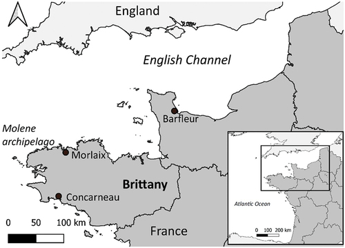
The distribution of L. digitata along European coasts ranges from the southern coast of Brittany, France (Quiberon Bay), to the northern coast of Norway (45.0°N to 71.5°N; 11.5°W to 27.0°E) (Davoult et al. 2011) (Figure 2). In France, kelp are found mainly in Brittany, especially at the Molène archipelago, where extraction of Laminariales represents 60–70% of national production (Vanhoutte-Brunier et al. 2016) and on which an economic sector depends. Most studies and quantitative estimates of kelp biomass were performed at two sites in Brittany – Morlaix and the Molène archipelago – which we considered as references (Gorman et al. 2013; Bajjouk et al. 2015) (section 2.4). Our study area includes the French side of the English Channel and the Brittany peninsula (Figure 2).

Figure 2. Study area location.

2.2. Kelp ES assessment

2.2.1. Literature review and classification of ES provided by kelp

An ES indicator is a parameter used to reflect the quality or quantity of an ES supply in order to monitor or communicate it (Hackbart et al. 2017). Its design and calculation will depend on the objectives, subject and scale of the study (Van Oudenhoven et al. 2018). A single indicator may not be sufficient to assess the different aspects of an ES. For instance, both carbon stocks and fluxes contribute to climate regulation which, as a consequence, could require using several indicators. To build a list of ES provided by kelps, we first performed a literature review with the keywords “kelp ecosystem services” in scientific literature databases (ISI web of Science, Google Scholar). Among the 18,600 search results, 139 publications were selected because they qualify or quantify an ES. The concept and typology of ES have evolved over time, along with an extensive debate about their adequacy (Haines-Young 2009). The Common International Classification of Ecosystem Services (CICES) has developed a general classification of ES, applicable to all ecosystems worldwide, to improve the comparison of results and methods among ES studies. Each kelp ES identified was classified according to the CICES latest version of ES classification (V5.1) (see Table 1). Finally, for each ES, we looked for whether a corresponding indicator already existed in the literature. If so, we included it directly in our study. Otherwise, we developed a new indicator (detailed below).

Table 1. Summary of the ecosystem services (ES) provided by kelp and examples of associated quantitative (Q) and non-quantitative (NQ) indicators. The ES are classified based on CICES v5.1. Bold text identifies the ES estimated and projected in this study. * indicates that the indicator is documented in the literature.

Section	Division	Group	Class of ES	CICES Code	Indicandum	Indicator and references	State
Provisioning	Biomass	Wild plants	Wild plants used for nutrition, material or energy	1.1.5	Kelp harvested for nutrition, cosmetics and pharmaceuticals	S1: Quantity of kelp biomass extracted (in tons per year) (Equation (1)(1) $Kelpbiomassextracted\left(intonsperyear\right)=kelpbiomass\times extractionquota$(1) )	Q
			Wild plants used for nutrition, material or energy	1.1.5.1	Alginate extracted for nutrition, cosmetics and pharmaceuticals	S2: Quantity of alginic acid (in tons per year) (Equation (2.1)(2.1) $Quantityofalginicacid\left(intonsperyear\right)=DW\times \frac{27}{100}$(2.1) )*	Q
		Wild animals	Wild animals used for nutrition, material or energy	1.1.6.1	Increase in fisheries	Increase in the local abundance of commercially valuable species (Vásquez et al. 2014)	Q
Regulation & Maintenance (biotic)	Transformation of biochemical or physical inputs to ecosystems	Mediation of wastes or toxic substances	Filtration/sequestration/storage/accumulation by organisms	2.1.1.1	Nutrient cycling	S3N: Quantity of nitrogen sequestered in kelp biomass (in tons per year) (Equation (3.1)(3.1) $Nitrogensequestred\left(intonsperyear\right)=kelpbiomass\times \frac{13}{100}\left(Eq.2.2\right)\times \frac{2.82}{100}$(3.1) )* S3P: Quantity of phosphorus sequestered in kelp biomass (in tons per year) (Equation (3.2)(3.2) $Phosphorussequestred(intonsperyear)=kelpbiomass\times \frac{13}{100}\left(Eq.2.2\right)\times \frac{0.32}{100}$(3.2) )*	Q
			Regulation of the chemical composition of atmosphere and oceans	2.2.6.1	Climate regulation	S4: Quantity of carbon sequestered in kelp biomass (in tons per year) (Equation (4)(4) $Carbonsequestred(intonsperyear)=kelpdistributionarea\times 3\left(Carbo{n}_{fixedperunitarea}\right)$(4) )*	Q
	Regulation of biochemical or physical inputs to ecosystems	Regulation of baseline flows	Control of erosion rates	2.2.1.1	Reduction of coastal erosion	Loss of sediment movement income (Arroyo et al. 2004)	Q
			Buffering and attenuation of mass movement	2.2.1.2	Wave damping and water velocity profile	Currents can be reduced by three time when kelp is present (Jackson and Winant 1983)	Q
			Hydrological cycle and water flow regulation	2.2.1.3	Coastal protection	S61: biophysical provision of coastal protection provided naturally by kelp (total length of the coastline, in km) S62: biophysical provision of protection coasts of urbanized provided naturally by kelp (total length of the coastline, in km)	Q
		Lifecycle maintenance, habitat and gene pool protection	Gamete dispersal	2.2.2.1	Dispersal via kelp rafts	Kelp-exported detritus is used as long-distance dispersal by some species (Krumhansl and Scheibling 2012)	NQ
			Seed dispersal	2.2.2.2
			Maintaining nursery populations and habitats	2.2.2.3	Provide space, food and protection for biota	Increase in abundance of adult fish associated with kelp (Bertocci et al. 2015)	Q
		Pest and disease control	Pest & invasive species control	2.2.3.1	Protection of endemic species	Reduction in kelp was associated with an increase in invasive species (Filbee-Dexter and Wernberg 2018)	NQ
			Disease control	2.2.3.2	Balance and complexity of the trophic chain	Kelp maintain a balanced health condition of the system (Campbell et al. 2014)	NQ
		Water conditions	Regulation of the chemical condition of salt water by living processes	2.2.5.2	Regulation of salt water conditions	S5: Quantity of O2released via kelp photosynthesis (in tons per year) (Equation (5)(5) $O_{2}released\hspace{0.17em}\left(intonsperyear\right)=Carbo{n}_{fixed}\times \frac{36}{12}$(5) )*	Q
					Acidification regulation	Kelp can increase aragonite saturation by 0.1 over 24 km^2 (Mongin et al. 2016)	NQ
Cultural	Direct and in-situ interactions (depend on presence in the environmental setting)	Physical and experiential interactions	Active or immersive interactions, activities	3.1.1.1	Ecotourism	Number of diving clubs & diving days per site near kelp (Blamey and Bolton 2018)	Q
			Passive or observational interactions, activities	3.1.1.2	Artistic inspiration	Number of artworks that represent kelp	NQ
		Intellectual and representative interactions	Scientific investigation, creation of traditional ecological knowledge	3.1.2.1	Research subject	Public investment in research funding (Bennett et al. 2016)	Q
			Education and training	3.1.2.2	Public awareness	Number of “kelp” news hits, Number of books on kelp sold (Duarte et al. 2008)	Q
			Culture, heritage	3.1.2.3	Cultural legacy of “goémoniers” (kelp harvesters)	Historical harvesting of kelp for agricultural land amendment and production of soda and iodine (Garineaud 2017)	NQ
	Indirect and remote interactions	Spiritual, symbolic interactions	Symbolic meaning	3.2.1.1	Local identity	Number of registered heritage species near kelp beds (Vanhoutte-Brunier et al. 2016)	Q

2.2.2. Quantification and mapping of ES indicators

We then classified the indicators into three classes of ES:

• (i) Non-quantitative: the ES can be identified, but no quantitative operational indicator can be developed due to no or few available data, or to a lack of knowledge of ecological processes

• (ii) Quantitative: the ES can be quantified using several indicators

• (iii) Spatial: the ES indicator is related to biomass and/or spatial dimension, and can be projected using ENM

We identified 20 ES provided by kelp (6 non-quantitative and 14 quantitative, among which 6 have spatial dimension) (Table 1).

Hereafter, we present the ES having a spatial dimension and retained to be projected by ENM as well as the related indicators. Indicators are calculated over a year.

2.2.2.1. Provisioning services

2.2.2.1.1. S1: kelp harvested for nutrition, cosmetics and pharmaceuticals

Because of the absence of data on the different uses (e.g. cosmetics and pharmaceuticals) of kelp, we considered the kelp biomass extracted (in tons of fresh weight) as an indicator of all the potential uses of kelp. This proxy is similar to what is practiced in fisheries (amount of biomass fished) or agriculture (amounts of crops extracted). To estimate this ES, we considered the current extraction quota of 20% of total kelp biomass, as recommended by Bajjouk et al. (2015). This quota was established in the Molène archipelago in Brittany, the country’s main area of kelp extraction. The indicator (in tons) was calculated at the national scale to quantify the potential supply of the ES, independent of the customs and uses specific to Brittany (Garineaud 2017). We assumed that kelp is extracted at sites that have at least a minimum threshold of abundance due to extraction limits (i.e. time, money and profitability).

(1) $Kelpbiomassextracted\left(intonsperyear\right)=kelpbiomass\times extractionquota$(1)

2.2.2.1.2. S2: alginate extracted for nutrition, cosmetics and pharmaceuticals

Kelp are harvested mainly for the high concentration of alginic acid in their tissues. This polysaccharide is precipitated to obtain alginate powder, which is used in agri-food, medical and cosmetic sectors as thickeners or as homogenising and gelling agents. We considered that the quantity of alginic acid (in tons) that can be extracted from kelp is an indicator of the alginate extracted for nutrition, cosmetics and pharmaceuticals service

The literature indicates that the alginic acid concentration ranges from 24% to 30% of kelp dry weight (DW) (Perez et al. 1992). The concentration varies among parts of the algae (i.e. stipe, blade and holdfast) by season and location (Goujon 2004). Therefore, we used a mean concentration of 27% of kelp DW to estimate the quantity of alginate that can be potentially extracted according to the quota (Equation (2.1)(2.1) $Quantityofalginicacid\left(intonsperyear\right)=DW\times \frac{27}{100}$(2.1) ).

As kelp is harvested as fresh weight (FW), we transformed FW into DW. Based on the literature, we used a mean of 13% of DW in FW (Gevaert et al. 2008; Laffoley and Grimsditch 2009; Chung et al. 2013) (Equation (2.2)(2.2) $DW=\hspace{0.17em}FW\times \frac{13}{100}$(2.2) ).

(2.1) $Quantityofalginicacid\left(intonsperyear\right)=DW\times \frac{27}{100}$(2.1)

where

(2.2) $DW=\hspace{0.17em}FW\times \frac{13}{100}$(2.2)

and FW = kelp biomass extracted according to Equation (1)(1) $Kelpbiomassextracted\left(intonsperyear\right)=kelpbiomass\times extractionquota$(1)

2.2.2.2. Regulation and maintenance services

2.2.2.2.1. S3 and S3P: nutrient cycling

Impacts of domestic and industrial wastewater discharge and diffuse pollution from agriculture are a particular concern for the health of marine biota (Fabricius et al. 2005). The quality of coastal water, monitored by multiple networks, depends on how wastewater is treated. The remaining untreated discharge is naturally buffered in the marine environment, within the limits of its ability, by specific organisms such as kelp, which can remove some contaminants (Camia et al. 2017). Filtration and sequestration of nitrogen (N) and phosphorus (P) can play an important role in mitigating eutrophication in coastal areas (Holdt and Edwards 2014). We estimated this ES by using an indicator that takes into account the quantities of N and P (in tons), which are critical nutrients in ecosystems (De Groot et al. 2002), potentially sequestered in kelp tissues.

To estimate these quantities, we assumed median values of 2.82% of DW for N concentration (Gevaert et al. 2008) and 0.32% of DW for P concentration of the entire kelp (Huang et al. 2005). We then used the conversion from FW to DW (Equation (2.2)(2.2) $DW=\hspace{0.17em}FW\times \frac{13}{100}$(2.2) ) to estimate the total quantity of N and P absorbed by kelp:

(3.1) $Nitrogensequestred\left(intonsperyear\right)=kelpbiomass\times \frac{13}{100}\left(Eq.2.2\right)\times \frac{2.82}{100}$(3.1)

(3.2) $Phosphorussequestred(intonsperyear)=kelpbiomass\times \frac{13}{100}\left(Eq.2.2\right)\times \frac{0.32}{100}$(3.2)

2.2.2.2.2. S4: climate regulation

Kelp beds are considered one of the most productive ecosystems on Earth, with a high turnover of biomass (Laffoley and Grimsditch 2009). They do not contribute to long-term carbon storage or mitigate against climate change, however, because they cannot store carbon below ground, and their turnover is extremely rapid, with most of their productivity being remineralised (Blamey and Bolton 2018), consumed, or decomposed (Krumhansl and Scheibling 2012). Nonetheless, kelp may play an indirect but significant role in carbon sequestration through photosynthesis by acting as carbon donors to recipient “blue carbon” habitats (e.g. seagrass meadows, deep sea and sediments), some of whose carbon may be stored in marine ecosystems over timescales relevant for sequestration (Fourqurean et al. 2012; Legge et al. 2020). Despite these uncertainties, carbon storage in kelp-dominated ecosystems is likely to be a function mainly of the standing biomass of kelp and associated understory algae; thus, we also considered short-term carbon sequestration. Thus, the ES indicator calculated is the amount of carbon sequestered by kelp (in tons).

It is difficult to compare the wide range of estimates of kelp net primary production and standing crop as the methods used vary greatly among species and studies (Laffoley and Grimsditch 2009). We used 3 kg C.m⁻².y⁻¹ for the quantity of carbon retained (i.e. the difference between carbon fixed and exuded) in dominant kelp ecosystems (Abdullah and Fredriksen 2004):

(4) $Carbonsequestred(intonsperyear)=kelpdistributionarea\times 3\left(Carbo{n}_{fixedperunitarea}\right)$(4)

The kelp distribution area is obtained from the outputs of the ENM detailed in section 2.3.3.3.3.

2.2.2.2.3. S5: regulation of salt water conditions

Due to high photosynthetic activity, kelp and macroalgae ecosystems release a massive quantity of dissolved oxygen (O₂) into the system. Water oxygenation is an essential function in marine ecosystems (Chen et al. 2012). Several items of the CICES classification can be related to this ecological process: breathing by animals, promoting the local presence of larval and juvenile fish (Smale et al. 2013), reinforcing lifecycle maintenance (Tempera et al. 2016), and providing a nursery service. The water oxygenation service also plays an indirect role in enhancing local fisheries (Campagne et al. 2015) and biodiversity of heritage interest for recreational activities and wildlife watching (Beaumont et al. 2008) such as snorkelling. Moreover, O₂ must be released to avoid eutrophication (Rabalais et al. 2009) by mediating waste, toxins, and other nuisances (Tempera et al. 2016). Water oxygenation also acts as an environmental buffer by modifying the chemical composition of the atmosphere and the ocean (Vásquez et al. 2014).

We classified “water oxygenation” as an indicator of “regulation of the chemical condition of salt water by living processes” ES (Filbee-Dexter and Wernberg 2018), which encompasses all the associated impacts, and whose indicator corresponds to the quantity of O2 (in tons) released by the kelp. As O₂ (in tons) is released through photosynthesis at the same time that carbon is fixed, we considered the rate of associated O₂ = carbon fixed $\times$ $\frac{36}{12}$ (Vassallo et al. 2013) and multiplied it by the quantity of carbon fixed by kelp:

(5) $O_{2}released\hspace{0.17em}\left(intonsperyear\right)=Carbo{n}_{fixed}\times \frac{36}{12}$(5)

2.2.2.2.4. S61 and S62: coastal protection

Kelp beds are known for their role in attenuating waves (Løvås and Tørum 2001; Blamey and Bolton 2018) and are assumed to protect the coastal shoreline from erosion and storms by changing the flow, sediment, and energy that pass through the system. However, the degree of ecosystem protection is non-linear (increasing as plant density increases), multifactorial and context-dependent (Pinsky et al. 2013). We estimated this ES from the presence of kelp at medium and high abundance classes (section 2.4) near the coastline. We used a geographical information system to measure the length of coastline along which a kelp seabed was located at a maximum distance of 1.5 km, using the “transect” function of QGIS software (QGIS Development Team 2021). For this first indicator, we considered the total length of coastline (in km) located within 1.5 km of kelp areas.

As the benefit of an ES depends on how local actors perceive it, two complementary approaches were used to assess this ES. The first indicator (S6₁) quantifies the biophysical provision of coastal protection provided naturally by kelp, regardless of the actual demand for it (Sousa et al. 2016). The second indicator (S6₂), which was limited to urbanised coastlines (e.g. houses, towns and roads), is highly relevant for local residents and actors who perceive the spatial extent of this ES (i.e. protecting the coastline and buildings against erosion). For this second indicator, we considered only the length of urbanised coastline (in km) located within 1.5 km of kelp areas. The nature of the coastline (artificial or natural) was uploaded from the French GéoLittoral (http://www.geolittoral.developpement-durable.gouv.fr/telechargement-en-ligne-donnees-geolittoral-a802.html). We assumed that the number of urban areas would not increase on the French coast of the North Atlantic due to the French “Coastline law” (articles L321 of the French Environmental Code).

2.3. Ecological niche models

We predicted future potential kelp species distribution in the context of climate change to explore its impacts on the delivery of ES under RCP2.6 (i.e. rapid mitigation of anthropogenic climate change and optimistic) and RCP8.5 (i.e. business-as-usual, high carbon emission scenario and pessimistic) scenarios of the Intergovernmental Panel on Climate Change for 2041–2050 (IPCC et al. 2018). To this end, we used a modelling framework dedicated to marine species distributions at the local scale (Ben Rais Lasram et al. 2020). The modelling procedure has two main steps: (i) a bioclimatic envelope model (BEM) applied at the global scale and calibrated with coarse-resolution climatic grids and (ii) a habitat model applied at the local scale and calibrated with fine-grained habitat variables.

2.3.1. Species data

We collected L. digitata data at two spatial extents: global scale (to run BEMs as an initial filter; section 2.3.3.3.3) and local scale (to run habitat models as a second filter; section 2.3.3.3.3). L. digitata occurrences at the global scale were uploaded from the Ocean Biogeographic Information System (https://obis.org/) and Global Biodiversity Information Facility (https://www.gbif.org/). For the local scale, occurrences obtained from Raybaud et al. (2013) were added to the global data.

Data was not processed at this stage since the ENM framework we used (Ben Rais Lasram et al. 2020) includes a procedure for homogenizing occurrences to reduce the influence of sampling bias and correcting erroneous records.

2.3.2. Environmental data

2.3.2.1. Global environmental data for the BEM

To calibrate the BEM, we used decadal means of temperature and salinity downloaded from the World Ocean Database (WOD) 2013 V2, from 1955 to 2012 (1955–1964, 1965–1974, 1975–1984, 1985–1994, 1995–2004 and 2005–2012), with a spatial resolution of 0.25°. The data were then interpolated to a five arcmin resolution (1/12°) using bilinear interpolation.

Most studies using ENM to predict species ranges consider two periods, usually the middle and end of the 21st century. We used the two scenarios RCP2.6 and RCP8.5, but for only one period (2041–2050), due to large uncertainties in changes in the socio-economic system that could occur (e.g. societal customs, uses of kelp ES).

Climate projections for the RCP2.6 and RCP8.5 scenarios for 2041–2050 were downloaded from three global circulation models from the Coupled Model Intercomparison Project Phase 5. We considered the 2005–2012 decade as the current baseline period and calculated projected anomalies between it and 2041–2050. These anomalies were then added to the observed mean temperatures and salinities for the same period of the WOD 2013 data.

2.3.2.2. Local environmental data for habitat models

We used five local habitat structure variables: depth, seafloor type, slope and slope orientations (eastwardness and northwardness). Data are available at EMODnet-bathymetry and EMODnet-seabed habitats (http://www.emodnet-seabedhabitats.eu/) and have a 250 m spatial resolution. The seafloor type was aggregated into eight EUNIS categories: rock, coarse sediment, sand, sandy mud, muddy sand, fine sand, mud, and fine mud. We did not consider turbidity, as no reliable future prediction of it was available. As light is a function of both depth and water turbidity, we used depth as a proxy for light, which decreases as depth increases (Van Son et al. 2020).

2.3.3. Modelling procedure

After processing data to reduce sampling effort bias and to generate pseudo-absences (see Hattab et al. 2014; Ben Rais Lasram et al. 2020; Marchand et al. 2020 for a complete overview of the underlying assumptions), we ran BEMs at the global scale using global temperature and salinity variables as a first climatic filter. To this end, eight algorithms were run individually with the “BIOMOD2” package (Thuiller et al. 2009) of R software (Team 2020): a generalized linear model, generalised additive model, multiple adaptive regression spline, boosted regression tree, random forest, classification tree analysis, flexible discriminant analysis, and artificial neural network. Each model was evaluated with a 3-fold cross-validation procedure by using a random sample of 75% of the initial data for calibration and the remaining 25% for validation. We used the true skill statistic (TSS) and continuous Boyce index (CBI) to assess the models’ predictive performance. Only algorithms that had CBI >0.5 for all three permutations (i.e. were resilient to occurrence permutations) were retained. A threshold that maximises the TSS score of the eight algorithms was used to generate current and predicted binary outputs (presence/absence) (Thuiller et al. 2009).

We then applied the second habitat filter using the procedure as for the first filter, but with habitat variables. A species was considered present when both filters predicted its presence. Finally, we used the projected temperatures and salinity for 2041–2050 according to the RCP2.6 and RCP8.5 scenarios to predict the potential future habitat for L. digitata according to each of the eight algorithms. To reduce uncertainties, rather than retaining the algorithm with the best TSS, we used the weighted average consensus method to generate final projections (Thuiller et al. 2009).

2.4. Relating ENM outputs to ES indicators

2.4.1. Biomass estimation

All the ES indicators used in this study have a spatial dimension related to the spatial distribution of kelps, that is, maps of probabilities of occurrence given by ENM outputs (probabilities that can be translated into binary occurrences by applying a threshold). Some of these ES indicators also required kelp biomass. To date, there is no data on the spatial distribution of kelp biomass available at the national level. Moreover, ENM project only distribution areas without considering biomass. Therefore, we estimated kelp biomass from maps of the probabilities of occurrence obtained by ENM. We assumed that higher probabilities of occurrence would imply environmental conditions strongly favourable for the species which could result in higher amounts of biomass produced. We also assumed that this relationship might not be linear and monotonous so we decided to build semi-quantitative indicator of biomass, that is, probabilities of occurrence were grouped into classes, to which we then assigned biomass values.

We classified pixels (of the maps of the probabilities of occurrence obtained by ENM) into four abundance classes based on their position in the distribution of the probability of occurrence (greater than zero probability), as follows:

• (i) Absent: pixels whose probability of occurrence lay below the first quartile (i.e. 1–42%), the related biomass is null.

• (ii) Low: pixels whose probability of occurrence lay between the first and second quartiles (i.e. 42–59%), the related biomass is B_low

• (iii) Medium: pixels whose probability of occurrence lay between the second and third quartiles (i.e. 59–83%), the related biomass is B_medium

• (iv) High: pixels whose probability of occurrence lay above the third quartile (i.e. 83–92%), the related biomass is B_high

We then assumed that the total biomass in an area (B_tot) could be assessed as:

(6) ${\mathrm{B}}_{\mathrm{t}\mathrm{o}\mathrm{t}}=\mathrm{r}\times ({\mathrm{P}}_{\mathrm{h}\mathrm{i}\mathrm{g}\mathrm{h}}\times {\mathrm{B}}_{\mathrm{h}\mathrm{i}\mathrm{g}\mathrm{h}}+\hspace{0.17em}{\mathrm{P}}_{\mathrm{m}\mathrm{e}\mathrm{d}\mathrm{i}\mathrm{u}\mathrm{m}}\times {\mathrm{B}}_{\mathrm{m}\mathrm{e}\mathrm{d}\mathrm{i}\mathrm{u}\mathrm{m}}+{\mathrm{P}}_{\mathrm{l}\mathrm{o}\mathrm{w}}\times {\mathrm{B}}_{\mathrm{l}\mathrm{o}\mathrm{w}})$(6)

where B_tot is the total biomass in an area, P is the number of pixels of the given abundance class, and r is the spatial resolution (here 0.09 km²).

We assigned a biomass to each class of probability of occurrence by overlapping the map of probability of occurrence of L. digitata obtained from ENM to two maps obtained from (Gorman et al. 2013) and (Bajjouk et al. 2015). (Gorman et al. 2013) and (Bajjouk et al. 2015) are two main references in the ecology of kelps and provide biomass in two sites that are, respectively, Morlaix and Molène archipelago. Gorman et al. (2013) estimated 56,634 t of L. digitata in an area of 130 km² at Morlaix, while (Bajjouk et al. 2015) estimated 98,401 t of L. digitata in an area of 214 km² at the Molène archipelago. At the Morlaix reference site, only medium and low abundance classes were present, with 321 and 5 pixels, respectively. The kelp biomass in the area of Morlaix could be assessed as:

(7) ${\mathrm{B}}_{\mathrm{M}\mathrm{o}\mathrm{r}\mathrm{l}\mathrm{a}\mathrm{i}\mathrm{x}}=\mathrm{r}\times \left(321{\mathrm{B}}_{\mathrm{m}\mathrm{e}\mathrm{d}\mathrm{i}\mathrm{u}\mathrm{m}}+5\times {\mathrm{B}}_{\mathrm{l}\mathrm{o}\mathrm{w}}\right)\hspace{0.17em}=\hspace{0.17em}56,634\hspace{0.17em}$(7)

We proceeded similarly with the biomass map of Gorman et al. (2013) at the Molène archipelago where the three abundance classes (high, medium and low) were present in 183, 456 and 798 pixels, respectively. The kelp biomass in the area of Molène could be assessed as:

(8) ${\mathrm{B}}_{\mathrm{M}\mathrm{o}\mathrm{l}\mathrm{e}\mathrm{n}\mathrm{e}}=\mathrm{r}\times \left(183\times {\mathrm{B}}_{\mathrm{h}\mathrm{i}\mathrm{g}\mathrm{h}}+456\times {\mathrm{B}}_{\mathrm{m}\mathrm{e}\mathrm{d}\mathrm{i}\mathrm{u}\mathrm{m}}+798\times {\mathrm{B}}_{\mathrm{l}\mathrm{o}\mathrm{w}}\right)=98,401\mathrm{t}$(8)

By overlapping the map of probability of occurrence of L. digitata obtained from ENM (for the current period) and the biomass map of Bajjouk et al. (2015) and Gorman et al. (2013), we affected an average biomass to the classes B_high, B_medium and B_low. Then, we averaged the values obtained for each biomass class and manually calibrated them in order to reach the correct values of s 7 and 8. The values retained are 2.0, 1.5 and 0.5 kg.m-² respectively for the high, medium, and low abundance classes. Then, we replaced these values in Equations (7)(7) ${\mathrm{B}}_{\mathrm{M}\mathrm{o}\mathrm{r}\mathrm{l}\mathrm{a}\mathrm{i}\mathrm{x}}=\mathrm{r}\times \left(321{\mathrm{B}}_{\mathrm{m}\mathrm{e}\mathrm{d}\mathrm{i}\mathrm{u}\mathrm{m}}+5\times {\mathrm{B}}_{\mathrm{l}\mathrm{o}\mathrm{w}}\right)\hspace{0.17em}=\hspace{0.17em}56,634\hspace{0.17em}$(7) and (8(8) ${\mathrm{B}}_{\mathrm{M}\mathrm{o}\mathrm{l}\mathrm{e}\mathrm{n}\mathrm{e}}=\mathrm{r}\times \left(183\times {\mathrm{B}}_{\mathrm{h}\mathrm{i}\mathrm{g}\mathrm{h}}+456\times {\mathrm{B}}_{\mathrm{m}\mathrm{e}\mathrm{d}\mathrm{i}\mathrm{u}\mathrm{m}}+798\times {\mathrm{B}}_{\mathrm{l}\mathrm{o}\mathrm{w}}\right)=98,401\mathrm{t}$(8) ) to check the correctness of our estimation. Our predictions have overestimated of 11.7% of the Morlaix results (Equation (7)(7) ${\mathrm{B}}_{\mathrm{M}\mathrm{o}\mathrm{r}\mathrm{l}\mathrm{a}\mathrm{i}\mathrm{x}}=\mathrm{r}\times \left(321{\mathrm{B}}_{\mathrm{m}\mathrm{e}\mathrm{d}\mathrm{i}\mathrm{u}\mathrm{m}}+5\times {\mathrm{B}}_{\mathrm{l}\mathrm{o}\mathrm{w}}\right)\hspace{0.17em}=\hspace{0.17em}56,634\hspace{0.17em}$(7) ), and underestimated of 23.1% of the Molène archipelago (Equation (8)(8) ${\mathrm{B}}_{\mathrm{M}\mathrm{o}\mathrm{l}\mathrm{e}\mathrm{n}\mathrm{e}}=\mathrm{r}\times \left(183\times {\mathrm{B}}_{\mathrm{h}\mathrm{i}\mathrm{g}\mathrm{h}}+456\times {\mathrm{B}}_{\mathrm{m}\mathrm{e}\mathrm{d}\mathrm{i}\mathrm{u}\mathrm{m}}+798\times {\mathrm{B}}_{\mathrm{l}\mathrm{o}\mathrm{w}}\right)=98,401\mathrm{t}$(8) ). Applying Equation (6)(6) ${\mathrm{B}}_{\mathrm{t}\mathrm{o}\mathrm{t}}=\mathrm{r}\times ({\mathrm{P}}_{\mathrm{h}\mathrm{i}\mathrm{g}\mathrm{h}}\times {\mathrm{B}}_{\mathrm{h}\mathrm{i}\mathrm{g}\mathrm{h}}+\hspace{0.17em}{\mathrm{P}}_{\mathrm{m}\mathrm{e}\mathrm{d}\mathrm{i}\mathrm{u}\mathrm{m}}\times {\mathrm{B}}_{\mathrm{m}\mathrm{e}\mathrm{d}\mathrm{i}\mathrm{u}\mathrm{m}}+{\mathrm{P}}_{\mathrm{l}\mathrm{o}\mathrm{w}}\times {\mathrm{B}}_{\mathrm{l}\mathrm{o}\mathrm{w}})$(6) gives a total biomass in the whole study area of 2,159,235 tons for the current period.

Finally, in order to validate this assessed biomass, we compared it to a biomass value found in Garineaud (2017). Indeed, Garineaud (2017) estimated that ca. 45,000 t of L. digitata are extracted each year in France (https://www.geolittoral.developpement-durable.gouv.fr/). As this quantity corresponds to 20% of the available total biomass (20% is the extraction quota according to Bajjouk et al. (2015)), we assumed that kelp biomass would equal five times the biomass extracted, that is, 225,000,000 t. Our assessed biomass overestimated the published values (Gorman et al. 2013; Bajjouk et al. 2015; Garineaud 2017) by 7%.

Once each biomass class is quantified for the current period, we used them to assess the future potential biomass by affecting each biomass class to the projected probabilities of occurrence under RCP2.6 and RCP8.5 scenarios for 2041–2050 and resulting from ENM. Finally, we estimated the average change in kelp biomass (expressed as a percentage) by subtracting the projected values under each RCP scenario from the current values (Table 2).

Table 2. Potential ES indicator values for the current period and projections for 2041–2050 under the RCP2.6 and RCP8.5 scenarios.

					Predictions for 2041–2050
				Current	RCP2.6		RCP8.5
Ecosystem service indicator	Code		Unit	Value	Value	Loss or gain	Value	Loss or gain
Total biomass of kelp			t fresh weight	2,159,235	829,890	−61.56%	729,540	−66.21%
Kelp biomass extraction	S1		t	377,793	112,491	−70.22%	34,011	−90.99%
Alginate extraction	S2		t	13,260	3,948	−70.22%	1,193	−90.99%
Nutrient cycling	S3N		t nitrogen	6,414	2,465	−61.56%	2,167	−66.21%
	S3P		t phosphorus	903.85	347.39	−61.56%	305.38	−66.21%
Carbon sequestration	S4		t	48,590	2,728	−43.85%	3,667	−24.53%
Water oxygenation	S5		t	14,577	8,185	−43.85%	11,001	−24.53%
Coastal protection (total vs. urbanised)	S61		km	930.65	259.85	−72.08%	36.83	−96.04%
	S62		km	76.64	10.17	−86.73%	0.77	−98.99%

2.4.2. ES quantification

Using ENM outputs, that is, species distribution (current and projected by 2041–2050 according to the RCP2.6 and RCP8.5 scenarios) and the related biomass, we calculated the ES current and future supply according to the eight equations of the indicators (sections 2.2.2.1.2.2.1 and 2.2.2.2) that we found in the literature or we developed in this work and that have a spatial dimension (Tables 1 and 2). To do that, we first replaced the “kelp biomass” or the “kelp distribution area” variables in each equation by the current biomass or the current distribution area in order to quantify the current supply of each ES. After that, we did similarly with the projected biomass or the projected distribution area, obtained from EMN, under both scenarios in order to quantify the future supply of each ES.

By subtracting the projected and current values, we assessed the potential loss or gain of ES supply (under RCP2.6 and RCP8.5 scenarios) as a response to climate change.

3. Results

3.1. Current and future variation of kelp biomass

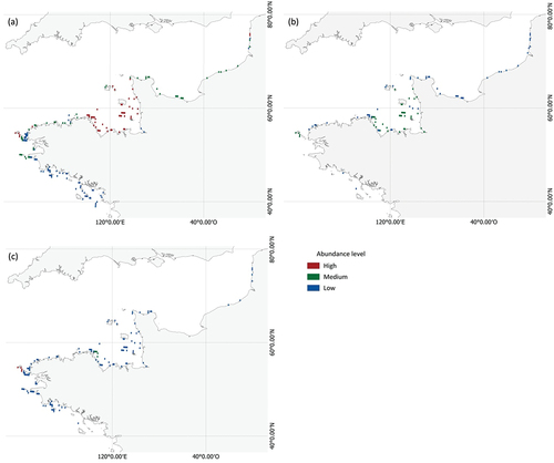
Current total L. digitata biomass was estimated at 2,159,235 t along the French coast (Table 2). Abundance was high from Concarneau to Barfleur, where 83% of the current estimated biomass was concentrated. This aggregation of kelp increased for 2041–2050 to 87% and 93% of the total predicted biomass from Barfleur to Concarneau for RCP2.6 and RCP8.5, respectively. Predictions for 2041–2050 revealed a global northward shift of L. digitata along the French coast. We predicted local extinction on the southern limit of its distribution (i.e. nearly complete disappearance south of Concarneau) and lower abundance along the northern limit (Figure 3). Overall, L. digitata had a similar range for the current period and both scenarios for 2041–2050. In contrast, biomass decreased greatly: by 62% under RCP2.6 and 66% under RCP8.5. The medium abundance class dominated under RCP2.6, while the low abundance class dominated under RCP8.5.

Figure 3. (a) Current and predicted distribution of Laminaria digitata grouped into abundance classes for 2041–2050 under (b) RCP2.6 and (c) RCP8.5 scenarios. Pixel resolution is magnified ten times. See Annexe 10 for maps in true resolution.

3.2. Inventory of ecosystem services provided by kelp and indicators

From the literature review, we identified 20 ES provided by kelp along the French coast (Table 1), of which six ES could be projected by ENM (Table 2).

In the provisioning section, among the three classes of ES identified, two indicandum “Kelp harvested for nutrition, cosmetics and pharmaceuticals” and “Alginate extracted for nutrition, cosmetics and pharmaceuticals” have been estimated by, respectively, the indicators “Quantity of kelp biomass extracted” and “Quantity of alginic acid” and projected.

In the regulation and maintenance section, among the eleven classes of ES identified, four indicandum “Nutrient cycling” (estimated by two indicators “Quantity of nitrogen sequestered in kelp biomass” and “Quantity of phosphorus sequestered in kelp biomass”), “Climate regulation” (estimated by one indicator “Quantity of carbon sequestered in kelp biomass”), “Coastal protection” (estimated by two indicators “Biophysical provision of coastal protection provided naturally by kelp” and “Biophysical provision of protection coasts of urbanized provided naturally by kelp”), and “Regulation of salt water conditions” (estimated by one indicator “Quantity of O2 released via kelp photosynthesis”) have been projected.

All the ES indicators estimated in this study express flows of ES ecological supply (i.e. amount per unit time), at the exception of the indicators related to “Coastal protection” that express an ES capacity (i.e. the potential of the coastal ecosystems to buffer extreme events and protect the coastline).

Finally, among the six classes of ES of the cultural section, none could be quantified and linked to a spatial dimension.

3.3. Current and projected potential values of kelp ES

Kelp ES are projected to decrease by 2041–2050, and more so under the RCP8.5 scenario, except for the carbon sequestration (S4) and water oxygenation (S5) indicators, both of which had the lowest projected decrease (24.53% and 43.85% under RCP8.5 and RCP2.6, respectively) (Table 2). The largest decrease in ES was protection of the urbanised coastline by kelp (S6₂) (98% and 86% under RCP8.5 and RCP2.6, respectively). The potential quantities of kelp extracted (S1) and alginic acid extracted (S2) both decreased by 70% under RCP2.6 and 91% under RCP8.5. The potential quantities of N (S3_N) and P (S3_P) recycled both decreased by 61% under RCP2.6 and 66% under RCP8.5. Several indicators were related to abundance and biomass, and thus to the spatial distribution of kelp. Thus, the locations where kelp were most affected were those with the greatest decrease in ES (except for indicator S6₁ and S6₂).

4. Discussion

Assessing species range shifts on global, regional or local scales as a response to climate change using ENM has been largely practiced the last two decades and IPBES together with IPCC warned on the urgent need to assess the impacts of climate change on ES. By combining ENM and Ecosystem Services indicators, our work offers an original methodological framework to deal with this issue.

To our knowledge, studies using ENM to predict or project ES provided by biodiversity are still rare. For example, Civantos et al. (2012) used ENM to project future spatial distribution of terrestrial vertebrates that control invertebrate and rodent pests in agricultural ecosystems. The substantial reduction of these “pest-control providers” spatial distributions as a response to climate change is expected to reduce the pest-control service they provide. In this paper, authors considered several species but only one ES. In the marine realm, Liquete et al. (2016) linked several biophysical and ecosystem modelling approaches to assess a set of ES in the Mediterranean Sea. Among these models, authors linked ENM to the lifecycle maintenance service of two fish species, the European hake Merluccius merluccius and the Atlantic bluefin tuna Thunnus thynnus, by identifying their spawning and nursery habitats but without any future projection.

Kelps, that have been revealed as increasingly threatened by climate change while providing numerous ecosystem services to humans, appear as a relevant example to apply our approach that consider several ES and projections under two climate scenarios for the middle of the century.

As it is difficult to assess all ES provided by kelp, our work doesn’t aim to estimate the whole bundle of ES but to demonstrate the relevance of the proposed methodological framework. We focused on six ES, among the 20 reviewed in the literature. These ES contribute directly to human well-being (i.e. provisioning and regulating services) and are projectable by ENM.

4.1. projected kelp distribution

In response to climate change, many taxa are expected to shift their ranges towards higher latitudes to remain in environments around their optimum temperature (Lenoir et al. 2020). Our results revealed that kelp would follow this trend in part, shifting their southern limit northward due to local extinctions by 2041–2050 for both RCP scenarios 2.6 and 8.5. Overall, our results agree with the trends observed by Raybaud et al. (2013) and Wilson et al. (2019), even though our results are related more to a decrease in biomass than to changes in spatial distribution. The expected absence of a northward shift of kelp populations due to increasing temperatures may be caused by the low availability of subtidal rocky shores along the northern coast of France. Brittany would progressively become the last refuge for kelp in France (Figure 3). This northern limit might decrease gene flow and adaptation to climate change, and possibly result in the disappearance of these populations and their ES, which could have strong impacts on human well-being and the overall functioning of coastal ecosystems.

Moreover, local loss of kelp biomass could occur more rapidly than projected by our models because we made the assumptions that kelp may disperse rapidly enough to keep pace with climate change. But kelp have a complex life cycle and, to date, little is known about their dispersal ability. Some authors postulate that kelp disperse rarely more than a few kilometres (Kinlan et al. 2005) while others suggest they may disperse over a longer distance (i.e. hundreds of km) under particular current conditions (Gutow and Thiel 2005).

4.2. impacts of climate change on kelp ES supply

Current evidence indicates that increasing pressure on ecosystems is likely to decrease the supply of ES (Schroter 2005; Metzger et al. 2006). For example, a decrease in the density and height of kelp canopies may hinder kelp’s contribution to reducing erosion on sandy coastlines (Jackson and Winant 1983). Our results showed that the decrease in kelp services is greater than the decrease in kelp biomass. As kelp form habitats, a shift in their distribution will disturb the coastal ecosystem’s biotic and abiotic components at multiple spatial extents. All species directly or indirectly related to kelp are likely to be impacted due to cascading effects (Lorentsen et al. 2010), including ES that have not been estimated here. As expected, the decrease is greater for the RCP8.5 pessimistic scenario, despite a similar projected kelp range between the current period and 2041–2050, but with decreasing biomass.

The weakening of kelp species and the resulting loss of biotic competitiveness could change the community composition to alternative and transitional ecosystem states (Filbee-Dexter and Wernberg 2018). This change could shift the dominant species on the bed of the ecosystem from L. digitata to another kelp species, such as Unidaria pinnatifida (considered invasive; (Véto-Leclerc 2019)) or Sacchoriza polyschides (the main competitor of L. digitata; (Engelen et al. 2011)), or to turf-dominated reefs (Gibson and Atkinson 2003). However, these transitional states will change the type of ecological functioning, which will support biophysical services that differ substantially in characteristics and quantity (Filbee-Dexter and Wernberg 2018). Even though L. digitata would no longer provide the ES, replacing them with other ecosystems could limit the loss of the ES provided.

In particular, we predicted a substantial decrease in kelp and alginate extraction services in 2041–2050, which agrees with the decrease in extractions that has been observed in Brittany for several decades (Davoult et al. 2011). The supply of these two ES requires only harvesting activity, which is possible only with a minimum density of kelp, in order to ensure the economic viability of this activity. In France, the current L. digitata extraction service is located exclusively in Brittany, which has the highest abundance of kelp. Thus, a 70–90% reduction in potentially extractable biomass would challenge the extraction service and the industry that has been built around it (as well as the resulting cultural services, such as heritage, identity, and scientific research). Our estimate of kelp and alginate extraction services at the scale of France was thus a potential estimate based on the current quota and practices. Thus, Brittany’s current supply of ES corresponds to 13% of the potential supply (S1 & S2) calculated at the national scale for the current period. This can be explained in part because no industry currently exploit kelp outside Britanny, despite its presence along other French coasts.

Despite a projected decrease in potential extraction of kelp of 70.22% and 90.99% under RCP2.6 and RCP8.5 scenarios, respectively, we projected that the supply of the extraction service will be 22% and 35% of the potential supply in Brittany and on a national scale, respectively. Thus, the potential to provide the extraction service will decrease less in the currently regulated areas than elsewhere. We can expect a disappearance of the kelp industry that will have major socio-cultural consequences in coastal regions. This requires increasing awareness of the importance of this ecosystem, as well as appropriate conservation measures.

4.3. Potential shortcomings of the study

The shortcomings of ENM are often discussed in the literature (Yalcin and Leroux 2017), which holds true for the biomass that we estimated. Translating a probability of occurrence into abundance or biomass is a major issue in ENM when the current georeferenced biomass is not available. Methods to estimate macroalgal standing crops in wild assemblages include in situ and remote sensing analyses. More recently, allometric equations have been developed to estimate kelp biomass (Stagnol et al. 2016; Van Son et al. 2020). At the local scale, previous studies have estimated standing kelp biomass at the Molène archipelago (Piriou et al. 1987; Arzel 1998; Bajjouk et al. 2015). However, differences in the methods used resulted in large differences in estimated stocks and distributions (Gevaert et al. 2008; Bajjouk et al. 2015). The method of translating quartiles of occurrence probability into biomass classes, calibrated using estimates from previous studies is obviously perfectible but it allows at least to assess the biomass where data is not available.

Although global georeferenced data have become more available recently for species occurrence data and environmental variables, sampling bias due to diverse and/or non-standardised monitoring surveys could increase the risk of oversampling (e.g. in accessible areas or areas with a long history of monitoring). Many regions lack reliable information on the structure and spatial extent of kelp beds, in part because shallow rocky reef habitats are logistically difficult to sample at large spatial scales (Teagle et al. 2017). Consequently, occurrence data often represent a biased sample of species populations, which can influence ENM calibration (Guillera-Arroita et al. 2015). We addressed these issues by combining referenced large-scale occurrences with independent local estimates of kelp biomass and by using a modelling framework that eliminates the influence of sampling bias (Ben Rais Lasram et al. 2020) while controlling the occurrences manually.

Ranges of many species may contract faster than models have predicted, as ENM are likely to be too conservative. For example, ENM do not consider changes in the distribution of favourable habitats caused by forcing factors such as increased sea level, water-column stratification, and sand displacement. Moreover, climate change can intensify the influence of other forcing factors, such as heatwaves (Wernberg et al. 2019), storms, invasive species, and water acidification (Valero et al. 2011; Harvey et al. 2013). Furthermore, an increase in temperature decreases O₂ and CO₂ solubility and influences photosynthesis (Raven et al. 2017). This could influence kelp’s growth, ability to reproduce and, more generally, physiology (Laffoley and Grimsditch 2009). Some studies argue that along with an increase in CO₂ concentrations, ocean warming may benefit kelp species. Kelp could adapt to increased atmospheric CO₂ by increasing growth rates (Harvey et al. 2013) and to increased temperature by increasing thermal optima for key physiological processes (Koch et al. 2013).

Multiple concurrent stressors (e.g. climate, anthropogenic and non-climate related) act synergistically rather than in isolation, so that the total impact is far greater than the sum of individual stressors (Harvey et al. 2013). Our models are thus likely to underestimate the impact of climate change on future dynamics of kelp, and kelp could lose distribution more rapidly than expected. As this study shows, the predicted decrease in kelp will also impact the associated food web, the structure and functioning of the dominant kelp ecosystem, and the ES provided that depend on it.

In this study, we considered a limited set of ES because of the limitations related to the quantification and mapping of ES. Moreover, considering the lack of available empirical or modelled data, and the difficulty to assess ES demand, our ES assessment was limited to the potential supply. Besides, we made strong assumptions that a decrease in biomass would lead to a decrease in ES supply although the relationship is not linear (Koch et al. 2009).

Finally, we didn’t consider social aspects related to ES supplied by kelps though they are important to address policy and societal issues.

4.4. Management implications

This study provides an assessment of the loss of ES provided by kelp as a consequence of climate change. Climate change along with kelp harvesting are considered as the most critical stressor of kelp beds (Araújo et al. 2016).

Indeed, kelp harvesting may fragment populations, and associated assemblages may not have time to recover (Christie et al. 1998). Kelp harvesting has been regulated for a long time (Frangoudes 2011), and despite tightly regulated practices, direct removal of kelp has considerable implications for population structure and ecosystem functioning, and the practices of extraction could accelerate the local extinction of kelp (Christie et al. 1998; Krumhansl and Scheibling 2012). Thus, climate change and harvesting act in synergy and could bring kelp beds to high biomass reduction or local extinction.

Unless we can counter the climate warming, that despite reductions in greenhouse gas emissions will reach at least 1.5° in the next decades (IPCC et al. 2018), there is an urgent need to sustainably manage kelp harvesting in order to mitigate the effects of climate change. Indeed, dense kelp beds where the harvesting pressure is limited could be more resilient to climate change.

To that aim, it would be necessary to update the current practiced quota harvesting (that is of 20% of total kelp biomass in France, Bajjouk et al. (2015)) and to allocate harvesting effort in a way that explicitly incorporate the influence of climate change based on future distribution areas and biomass.

This requires more knowledge on the life history traits and physiology of the specie and its plasticity and adaptation to climate change as well as on its dispersal capacities. This could help to explore whether kelp would disperse rapidly enough to keep pace with climate and to identify future hotspot areas where harvesting effort could be allocated. This could avoid bringing the specie to local extinction in areas where biomass is expected to decrease or populations to be isolated.

Another option that could reduce the harvesting pressure on kelp could be aquaculture. Kelp aquaculture is a promising solution to maintain the provisioning services (Peteiro 2018), but it remains in its infancy in Europe and will have to overcome several constraints to become a reliable alternative to the biomass supplied by wild harvesting (Gentry et al. 2020). In addition, kelp aquaculture could reduce the extraction pressure on wild populations and provide certain ES to fulfil several strategies for adapting to climate change (Chung et al. 2017), such as nutrient absorption (Gentry et al. 2020). On the other hand, kelp cultivation could negatively impact local ES, however, as they could change local patterns of water flow and cause organic enrichment of sediments (Krumhansl and Scheibling 2012). Impact assessments are required to explore the sustainability of such an activity.

Finally, by integrating explicitly kelp forests as a vulnerable habitat in the European Habitats Directive (instead of considering them as simply components of “reef” habitats (Beck and Airoldi 2007; Teagle et al. 2017)), they could benefit from conservation measures as a priority. Conservation measures include harvesting control and also design of marine protected areas that take into account current and future kelp distribution areas.

Overall, using ENM to project future ES supply will help to manage kelps by opting for alternative uses combined with conservation measures.

5. Conclusion and perspective

While conservative ecosystem-based management is required to harvest marine resources sustainably, baseline knowledge of the structure and functioning of kelp ecosystems at the regional scale is currently lacking (Smale et al. 2013). This creates an urgent need to develop rapid and effective methodological frameworks that can guide and monitor management strategies under the European Union’s Marine Strategy Framework Directive by taking into account the effects of climate change. In this context, our approach combines Ecological Niche Models and ecosystem services indicators to assess the potential loss of ES supplied by kelps that humans would undergo as a response to climate change. This loss assessment could help to convince decision makers to better manage kelp beds in order to mitigate the effects of climate change.

Perspectives for future studies include additional simulations based on general social-economic trends (e.g. “sustainable well-being” vs. “fossil-fuelled development”) that will result in changing the path of the use and supply of marine ES (Cabral et al. 2015). Aiming for sustainable use of ES challenges the ability to relate biodiversity to ecosystem functions and services in integrated mechanistic models. Trait-based models, based on quantitative relationships between trait-based metrics and ES provided by an ecosystem, are a promising tool for adjusting our methodological framework (Lavorel et al. 2017). Using the ecological features of kelp, such as plant density, the length of the thallus (Van Son et al. 2020) and how kelp interact with other species (Thuiller 2004) and/or respond to pressures, could provide insights into how the species provides ES and thus reduce uncertainty in ES projections.

Geolocation information

The study site of this paper is located on the French coast, within the spatial extent : −5.42,47.05 : 2.54,51.1 (WGS 84).

Acknowledgements

The authors would like to acknowledge the University of Littoral Opal Coast (ULCO) that funded this work.

Disclosure statement

No potential conflict of interest was reported by the author(s).

Additional information

Funding

This work was supported by the University of Littoral Opal Coast (ULCO).

References

- Abdullah MI, Fredriksen S. 2004. Production, respiration and exudation of dissolved organic matter by the kelp Laminaria hyperborea along the west coast of Norway. J Mar Biolog Assoc UK. 84(5):887–894. doi:10.1017/S002531540401015Xh.
- Araújo RM, Assis J, Aguillar R, Airoldi L, Bárbara I, Bartsch I, Bekkby T, Christie H, Davoult D, Derrien-Courtel S, et al. 2016. Status, trends and drivers of kelp forests in Europe: an expert assessment. Biodivers Conserv. 25(7):1319–1348. doi:10.1007/s10531-016-1141-7.
- Arkema KK, Guannel G, Verutes G, Wood SA, Guerry A, Ruckelshaus M, Kareiva P, Lacayo M, Silver JM. 2013. Coastal habitats shield people and property from sea-level rise and storms. Nat Clim Chang. 3(10):913–918. doi:10.1038/nclimate1944.
- Arroyo NL, Maldonado M, Pérez-Portela R, Benito J. 2004. Distribution patterns of meiofauna associated with a sublittoral Laminaria bed in the Cantabrian Sea (north-eastern Atlantic). Mar Biol. 144(2):231–242. doi:10.1007/s00227-003-1191-8.
- Arzel P. 1998. Les laminaires sur les côtes bretonnes: évolution de l’exploitation et de la flottille de pêche, état actuel et perspectives. France: Editions Ifremer.
- Assis J, Araújo MB, Serrão EA. 2018. Projected climate changes threaten ancient refugia of kelp forests in the North Atlantic. Glob Chang Biol. 24(1):e55–e66. doi:10.1111/gcb.13818.
- Bajjouk T, Rochette S, Laurans M, Ehrhold A, Hamdi A, Le Niliot P. 2015. Multi-Approach mapping to help spatial planning and management of the kelp species L. digitata and L. hyperborea: Case study of the Molène Archipelago, Brittany. J Sea Res. 100:2–21. doi:10.1016/j.seares.2015.04.004.
- Barbier EB, Baumgärtner S, Chopra K, Costello C, Duraiappah A, Hassan R, Kinzig A, Lehman M, Pascual U, Polasky S. 2009. The valuation of ecosystem services. Biodiversity, Ecosystem Functioning, and Human Wellbeing: An Ecological and Economic Perspective. p. 248–262.
- Bartsch I, Wiencke C, Bischof K, Buchholz CM, Buck BH, Eggert A, Feuerpfeil P, Hanelt D, Jacobsen S, Karez R, et al. 2008. The genus Laminaria sensu lato: Recent insights and developments. Eur J Phycol. 43(1):1–86. doi:10.1080/09670260701711376.
- Beaumont NJ, Austen MC, Mangi SC, Townsend M. 2008. Economic valuation for the conservation of marine biodiversity. Mar Pollut Bull. 56(3):386–396. doi:10.1016/j.marpolbul.2007.11.013.
- Beck M, Airoldi L. 2007. Loss, Status and Trends for Coastal Marine Habitats of Europe. In: Gibson RN; Atkinson RJA Gordon JDM. Oceanography and Marine Biology. Vol. 20074975, CRC Press; pp. 345–405. doi:10.1201/9781420050943.ch7
- Bekkby T, Rinde E, Erikstad L, Bakkestuen V. 2009. Spatial predictive distribution modelling of the kelp species Laminaria hyperborea. ICES J Mar Sci. 66(10):2106–2115. doi:10.1093/icesjms/fsp195.
- Bekkby T, Smit C, Gundersen H, Rinde E, Steen H, Tveiten L, Gitmark JK, Fredriksen S, Albretsen J, Christie H. 2019. The Abundance of Kelp is Modified by the Combined Impact of Depth, Waves and Currents. Front Mar Sci. 6:475. doi:10.3389/fmars.2019.00475.
- Ben Rais Lasram F, Hattab T, Nogues Q, Beaugrand G, Dauvin JC, Halouani G, Le Loc’-H F, Niquil N, Leroy B. 2020. An open-source framework to model present and future marine species distributions at local scale. Ecol Inform. 59:101130. doi:10.1016/j.ecoinf.2020.101130.
- Bennett S, Wernberg T, Connell SD, Hobday AJ, Johnson CR, Poloczanska ES. 2016. The ‘Great Southern Reef’: Social, ecological and economic value of Australia’s neglected kelp forests. Null. 67(1):47–56. doi:10.1071/MF15232.
- Bertocci I, Araújo R, Oliveira P, Sousa-Pinto I. 2015. Potential effects of kelp species on local fisheries. J Appl Ecol. 52(5):1216–1226. doi:10.1111/1365-2664.12483.
- Blamey LK, Bolton JJ. 2018. The economic value of South African kelp forests and temperate reefs: Past, present and future. J Mar Syst. 188:172–181. doi:10.1016/j.jmarsys.2017.06.003.
- Bolton JJ, Lüning K. 1982. Optimal growth and maximal survival temperatures of Atlantic Laminaria species (Phaeophyta) in culture. Mar Biol. 66(1):89–94. doi:10.1007/BF00397259.
- Byrne M, Foo SA, Ross PM, Putnam HM. 2020. Limitations of cross-and multigenerational plasticity for marine invertebrates faced with global climate change. Glob Chang Biol. 26(1):80–102. doi:10.1111/gcb.14882.
- Cabral P, Levrel H, Schoenn J, Thiebaut E, Le Mao P, Mongruel R, Rollet C, Dedieu K, Carrier S, Morisseau F. 2015. Marine habitats ecosystem service potential: a vulnerability approach in the Normand-Breton (Saint Malo) Gulf, France. Ecosyst Serv. 16:306–318. doi:10.1016/j.ecoser.2014.09.007.
- Camia A, Robert N, Pilli R, Mubareka S, Blujdea V, Araujo R, Merino NM, Hoepffner N, Casey J, Doerner H 2017. Report on current biomass supply and technical potential with a focus on Europe.
- Campagne CS, Salles J-M, Boissery P, Deter J. 2015. The seagrass Posidonia oceanica: Ecosystem services identification and economic evaluation of goods and benefits. Mar Pollut Bull. 97(1–2):391–400. doi:10.1016/j.marpolbul.2015.05.061.
- Campbell AH, Vergés A, Steinberg PD. 2014. Demographic consequences of disease in a habitat-forming seaweed and impacts on interactions between natural enemies. Ecology. 95(1):142–152. doi:10.1890/13-0213.1.
- Chen B, He G, Yang J, Zhang J, Su M, Qi J. 2012. Evaluating ecological and economic benefits of a low-carbon industrial park based on millennium ecosystem assessment framework. Sci World J. 2012:1–5. doi:10.1100/2012/909317.
- Christie H, Fredriksen S, Rinde E. 1998. Regrowth of kelp and colonization of epiphyte and fauna community after kelp trawling at the coast of Norway. In: Recruitment, colonization and physical-chemical forcing in marine biological systems. Springer Netherlands; pp. 49–58. doi:10.1007/978-94-017-2864-5_4
- Chung IK, Oak JH, Lee JA, Shin JA, Kim JG, Park K-S. 2013. Installing kelp forests/seaweed beds for mitigation and adaptation against global warming: Korean project overview. ICES J Mar Sci. 70(5):1038–1044. doi:10.1093/icesjms/fss206.
- Chung IK, Sondak CFA, Beardall J. 2017. The future of seaweed aquaculture in a rapidly changing world. Eur J Phycol. 52(4):495–505. doi:10.1080/09670262.2017.1359678.
- Civantos E, Thuiller W, Maiorano L, Guisan A, Araújo MB. 2012. Potential impacts of climate change on ecosystem services in Europe: the case of pest control by vertebrates. BioScience. 62(7):658–666. doi:10.1525/bio.2012.62.7.8.
- Costanza R, Limburg K, Naeem S, O’-Neill RV, Paruelo J, Raskin RG, Sutton P. 1997. The value of the world’s ecosystem services and natural capital. Nature. 387(6630):253–260. doi:10.1038/387253a0.
- Davoult D, Engel CR, Arzel P, Knoch D, Laurans M. 2011. Environmental factors and commercial harvesting: Exploring possible links behind the decline of the kelp Laminaria digitata in Brittany, France. CBM-Cah Biol Mar. 52(4):429.
- Dayton PK. 1985. Ecology of kelp communities. Annu Rev Ecol Syst. 16(1):215–245. doi:10.1146/annurev.es.16.110185.001243.
- De Groot RS, Wilson MA, Boumans RM. 2002. A typology for the classification, description and valuation of ecosystem functions, goods and services. Ecol Econ. 41(3):393–408. doi:10.1016/S0921-8009(02)00089-7.
- Dendoncker N, Boeraeve F, Crouzat E, Dufrêne M, König A, Barnaud C. 2018. How can integrated valuation of ecosystem services help understanding and steering agroecological transitions? Ecol Soc. 23(1). doi:10.5751/ES-09843-230112.
- Duarte CM, Dennison WC, Orth RJ, Carruthers TJ. 2008. The charisma of coastal ecosystems: Addressing the imbalance. Estuaries Coasts. 31(2):233–238. doi:10.1007/s12237-008-9038-7.
- Duffy GA, Chown SL. 2017. Explicitly integrating a third dimension in marine species distribution modelling. Mar Ecol Prog Ser. 564:1–8. doi:10.3354/meps12011.
- Edgar GJ, Barrett NS, Graddon DJ, Last PR. 2000. The conservation significance of estuaries: a classification of Tasmanian estuaries using ecological, physical and demographic attributes as a case study. Biol Conserv. 92(3):383–397. doi:10.1016/S0006-3207(99)00111-1.
- Engelen AH, Lévèque L, Destombe C, Valero M. 2011. Spatial and temporal patterns of recovery of low intertidal Laminaria digitata after experimental spring and autumn removal. CBM-Cah Biol Mar. 52(4):441.
- Fabricius K, De’-Ath G, McCook L, Turak E, Williams DM. 2005. Changes in algal, coral and fish assemblages along water quality gradients on the inshore great barrier reef. Mar Pollut Bull. 51(1–4):384–398. doi:10.1016/j.marpolbul.2004.10.041.
- Feng X, Park DS, Walker C, Peterson AT, Merow C, Papeş M. 2019. A checklist for maximizing reproducibility of ecological niche models. Nat Ecol Evol. 3(10):1382–1395. doi:10.1038/s41559-019-0972-5.
- Filbee-Dexter K, Wernberg T. 2018. Rise of turfs: a new battlefront for globally declining kelp forests. BioScience. 68(2):64–76. doi:10.1093/biosci/bix147.
- Fourqurean JW, Duarte CM, Kennedy H, Marbà N, Holmer M, Mateo MA, Apostolaki ET, Kendrick GA, Krause-Jensen D, McGlathery KJ. 2012. Seagrass ecosystems as a globally significant carbon stock. Nat Geosci. 5(7):505–509. doi:10.1038/ngeo1477.
- Frangoudes K. 2011. Seaweeds fisheries management in France, Japan, Chile and Norway. CBM-Cah Biol Mar. 52(4):517.
- Fraser CI. 2012. Is bull-kelp kelp? the role of common names in science. N Z J Mar Freshwater Res. 46(2):279–284. doi:10.1080/00288330.2011.621130.
- Garineaud C. 2017. Récolter la mer: Des savoirs et des pratiques des collecteurs d’algues à la gestion durable des ressources côtières dans le Finistère (Bretagne) [doctoral dissertation]. France: Museum national d’histoire naturelle-MNHN PARIS.
- Gentry RR, Alleway HK, Bishop MJ, Gillies CL, Waters T, Jones R. 2020. Exploring the potential for marine aquaculture to contribute to ecosystem services. Rev Aquac. 12(2):499–512. doi:10.1111/raq.12328.
- Gevaert F, Janquin M-A, Davoult D. 2008. Biometrics in Laminaria digitata: a useful tool to assess biomass, carbon and nitrogen contents. J Sea Res. 60(3):215–219. doi:10.1016/j.seares.2008.06.006.
- Gibson R, Atkinson R. 2003. The effects of sedimentation on rocky coast assemblages. Oceanogr Mar Biol. 41:161–236.
- Gómez-Baggethun E, Martín-López B, Barton D, Braat L, Saarikoski H, Kelemen E, García-Llorente M, van den Bergh J, Arias P, Berry P. 2014. State-Of-The-Art report on integrated valuation of ecosystem services. EU FP7 OpenNess Project Deliverable. 4:1–33.
- Gorman D, Bajjouk T, Populus J, Vasquez M, Ehrhold A. 2013. Modeling kelp forest distribution and biomass along temperate rocky coastlines. Mar Biol. 160(2):309–325. doi:10.1007/s00227-012-2089-0.
- Goujon I. 2004. Les alginates, excipients d’origine marine utilisés dans l’industrie pharmaceutique: applications à la synthèse d’un gel chimique [doctoral dissertation]. France: UHP-Université Henri Poincaré.
- Gregr EJ, Palacios DM, Thompson A, Chan KMA. 2019. Why less complexity produces better forecasts: an independent data evaluation of kelp habitat models. Ecography. 42(3):428–443. doi:10.1111/ecog.03470.
- Guillera-Arroita G, Lahoz-Monfort JJ, Elith J, Gordon A, Kujala H, Lentini PE, McCarthy MA, Tingley R, Wintle BA. 2015. Is my species distribution model fit for purpose? Matching data and models to applications. Glob Ecol Biogeogr. 24(3):276–292. doi:10.1111/geb.12268.
- Gutow L, Thiel M. 2005. The ecology of rafting in marine crustaceans, 12. Crustaceologen-Tagung, 17.-20.
- Hackbart VCS, de Lima GTNP, dos Santos RF. 2017. Theory and practice of water ecosystem services valuation: Where are we going? Ecosyst Serv. 23(C):218–227. doi:10.1016/j.ecoser.2016.12.010.
- Haines-Young R. 2009. Land use and biodiversity relationships. Land Use Policy. 26:S178–S186. doi:10.1016/j.landusepol.2009.08.009
- Harvey BP, Gwynn-Jones D, Moore PJ. 2013. Meta-Analysis reveals complex marine biological responses to the interactive effects of ocean acidification and warming. Ecol Evol. 3(4):1016–1030. doi:10.1002/ece3.516.
- Hattab T, Albouy C, Lasram FBR, Somot S, Le Loc’-H F, Leprieur F. 2014. Towards a better understanding of potential impacts of climate change on marine species distribution: a multiscale modelling approach. Glob Ecol Biogeogr. 23(12):1417–1429. doi:10.1111/geb.12217.
- Hawkins SJ, Hartnoll RG. 1985. Factors determining the upper limits of intertidal canopy-forming algae. Mar Ecol Prog Ser. 20(3):265–271. doi:10.3354/meps020265.
- Holdt SL, Edwards MD. 2014. Cost-Effective IMTA: a comparison of the production efficiencies of mussels and seaweed. J Appl Phycol. 26(2):933–945. doi:10.1007/s10811-014-0273-y.
- Huang D, Huang X, Yue W. 2005. Contents of TN, TP in macroalgae and its significance for remediation of coastal environment. J Oceanogr Taiwan Strait. 24(3):316.
- IPCC, Intergovernmental Panel on Climate Change. Masson-Delmotte V, Zhai P, Pörtner HO, Roberts D, Skea J, Shukla PR, Pirani A, Moufouma-Okia W, Péan C, et al. 2018. Summary for Policymakers. In: Global warming of 1.5°C. An IPCC Special Report on the impacts of global warming of 1.5°C above pre-industrial levels and related global greenhouse gas emission pathways, in the context of strengthening the global response to the threat of climate change, sustainable development, and efforts to eradicate poverty. Geneva, Switzerland: World Meteorological Organization. p. 32
- Jackson GA, Winant CD. 1983. Effect of a kelp forest on coastal currents. Cont Shelf Res. 2(1):75–80. doi:10.1016/0278-4343(83)90023-7.
- Jonsson PR, Kotta J, Andersson HC, Herkül K, Virtanen E, Sandman AN, Johannesson K. 2018. High climate velocity and population fragmentation may constrain climate-driven range shift of the key habitat former Fucus vesiculosus. Null. 24(7):892–905. doi:10.1111/ddi.12733.
- Kadykalo AN, López-Rodriguez MD, Ainscough J, Droste N, Ryu H, Ávila-Flores G, Le Clec’-H S, Muñoz MC, Nilsson L, Rana S, et al. 2019. Disentangling ‘ecosystem services’ and ‘nature’s contributions to people’. Ecosyst People. 15(1):269–287. doi:10.1080/26395916.2019.1669713.
- Karsten U. 2007. Research note: Salinity tolerance of arctic kelps from spitsbergen. Phycol Res. 55(4):257–262. doi:10.1111/j.1440-1835.2007.00468.x.
- Kinlan BP, Gaines SD, Lester SE. 2005. Propagule dispersal and the scales of marine community process. Null. 11(2):139–148. doi:10.1111/j.1366-9516.2005.00158.x.
- Koch EW, Barbier EB, Silliman BR, Reed DJ, Perillo GM, Hacker SD, Granek EF, Primavera JH, Muthiga N, Polasky S. 2009. Non-Linearity in ecosystem services: Temporal and spatial variability in coastal protection. Front Ecol Environ. 7(1):29–37. doi:10.1890/080126.
- Koch M, Bowes G, Ross C, Zhang X-H. 2013. Climate change and ocean acidification effects on seagrasses and marine macroalgae. Glob Chang Biol. 19(1):103–132. doi:10.1111/j.1365-2486.2012.02791.x.
- Krause-Jensen D, Duarte CM. 2016. Substantial role of macroalgae in marine carbon sequestration. Nat Geosci. 9(10):737–742. doi:10.1038/ngeo2790.
- Krause-Jensen D, Lavery P, Serrano O, Marbà N, Masque P, Duarte CM. 2018. Sequestration of macroalgal carbon: the elephant in the blue carbon room. Biol Lett. 14(6):20180236. doi:10.1098/rsbl.2018.0236.
- Krumhansl K, Scheibling R. 2012. Production and fate of kelp detritus. Mar Ecol Prog Ser. 467:281–302. doi:10.3354/meps09940.
- Krumhansl KA, Okamoto DK, Rassweiler A, Novak M, Bolton JJ, Cavanaugh KC, Connell SD, Johnson CR, Konar B, Ling SD. 2016. Global patterns of kelp forest change over the past half-century. Proc Natl Acad Sci. 113(48):13785–13790. doi:10.1073/pnas.1606102113.
- Laffoley D, Grimsditch GD. 2009. The management of natural coastal carbon sinks. Iucn. Gland (Switzerland): IUCN; 53 pp.
- Lavorel S, Bayer A, Bondeau A, Lautenbach S, Ruiz-Frau A, Schulp N, Seppelt R, Verburg P, van Teeffelen A, Vannier C. 2017. Pathways to bridge the biophysical realism gap in ecosystem services mapping approaches. Ecol Indic. 74:241–260. doi:10.1016/j.ecolind.2016.11.015.
- Legge O, Johnson M, Hicks N, Jickells T, Diesing M, Aldridge J, Andrews J, Artioli Y, Bakker DC, Burrows MT. 2020. Carbon on the Northwest European shelf: Contemporary budget and future influences. Front Mar Sci. 7:143. doi:10.3389/fmars.2020.00143.
- Lenoir J, Bertrand R, Comte L, Bourgeaud L, Hattab T, Murienne J, Grenouillet G. 2020. Species better track climate warming in the oceans than on land. Nat Ecol Evol. 4(8):1–16.
- Li SB, Chen PH, Huang JS, Hsueh ML, Hsieh LY, Lee CL, Lin HJ. 2018. Factors regulating carbon sinks in mangrove ecosystems. Glob Chang Biol. 24(9):4195–4210. doi:10.1111/gcb.14322.
- Liquete C, Piroddi C, Macías D, Druon JN, Zulian G. 2016. Ecosystem services sustainability in the Mediterranean Sea: assessment of status and trends using multiple modelling approaches. Sci Rep. 6(1):1–14.
- Lorentsen SH, Sjøtun K, Grémillet D. 2010. Multi-Trophic consequences of kelp harvest. Biol Conserv. 143(9):2054–2062. doi:10.1016/j.biocon.2010.05.013.
- Løvås SM, Tørum A. 2001. Effect of the kelp Laminaria hyperborea upon sand dune erosion and water particle velocities. Coast Eng. 44(1):37–63. doi:10.1016/S0378-3839(01)00021-7.
- Lüning K. 1990. Seaweeds: Their environment, biogeography, and ecophysiology. John Wiley & Sons.
- Marchand ML, Hattab T, Niquil N, Albouy C, Loc’-H FL, Lasram FBR. 2020. Climate change in the Bay of Biscay: Changes in spatial biodiversity patterns could be driven by the arrivals of southern species. Mar Ecol Prog Ser. 647:17–31. doi:10.3354/meps13401.
- McLean M, Mouillot D, Maureaud AA, Hattab T, MacNeil MA, Goberville E, Lindegren M, Engelhard G, Pinsky M, Auber A. 2021. Disentangling tropicalization and deborealization in marine ecosystems under climate change. Curr Biol. 31(21):4817–4823. doi:10.1016/j.cub.2021.08.034.
- [MEA] Millennium Ecosystem Assessment. 2005. Ecosystems and human well-being. Vol. 5. Washington, DC: Island press.
- Melo-Merino SM, Reyes-Bonilla H, Lira-Noriega A. 2020. Ecological niche models and species distribution models in marine environments: a literature review and spatial analysis of evidence. Ecol Modell. 415:108837. doi:10.1016/j.ecolmodel.2019.108837.
- Metzger M, Rounsevell MDA, Acosta-Michlik L, Leemans R, Schröter D. 2006. The vulnerability of ecosystem services to land use change. Agric Ecosyst Environ. 114(1):69–85. doi:10.1016/j.agee.2005.11.025.
- Mongin M, Baird ME, Hadley S, Lenton A. 2016. Optimising reef-scale CO2 removal by seaweed to buffer ocean acidification. Environ Res Lett. 11(3):034023. doi:10.1088/1748-9326/11/3/034023.
- Morley JW, Selden RL, Latour RJ, Frölicher TL, Seagraves RJ, Pinsky ML. 2018. Projecting shifts in thermal habitat for 686 species on the North American continental shelf. PloS One. 13(5):e0196127. doi:10.1371/journal.pone.0196127.
- O’-Brien JM, Scheibling RE. 2016. Nipped in the bud: Mesograzer feeding preference contributes to kelp decline. Ecology. 97(7):1873–1886. doi:10.1890/15-1728.1.
- Pascual U, Balvanera P, Díaz S, Pataki G, Roth E, Stenseke M, Watson RT, Başak Dessane E, Islar M, Kelemen E, et al. 2017. Valuing nature’s contributions to people: the IPBES approach. Curr Opin Environ Sustain. 26–27:7–16. doi:10.1016/j.cosust.2016.12.006.
- Perez R, Kaas R, Campello F, Arbault S, Barbaroux O. 1992. La Culture des algues marines dans le monde. France: Ifremer Editions; 637 pp.
- Peteiro C. 2018. Alginate production from marine macroalgae, with emphasis on kelp farming. In: Rehm BHA Moradali MF, editors. Alginates and their biomedical applications. Vol. 11. Springer Singapore; p. 27–66. doi:10.1007/978-981-10-6910-9_2
- Pinsky ML, Worm B, Fogarty MJ, Sarmiento JL, Levin SA. 2013. Marine taxa track local climate velocities. Science. 341(6151):1239–1242. doi:10.1126/science.1239352.
- Piriou J-Y, Youenou G, Dreves L, Chapron V. 1987. Cartographie de la végétation marine côtière sur le littoral Bas-Léonard (Finistère Nord). France: Ifremer Edition; 53 pp.
- Pörtner HO, Scholes RJ, Agard J, Archer E, Arneth A, Bai X, Barnes D, Burrows M, Chan L, Cheung WL 2021. IPBES-IPCC co-sponsored workshop report on biodiversity and climate change.
- QGIS Development Team. 2021. QGIS geographic information system. Open Source Geospatial Foundation Project. http://qgis.osgeo.org.
- Rabalais NN, Turner RE, Díaz RJ, Justić D. 2009. Global change and eutrophication of coastal waters. ICES J Mar Sci. 66(7):1528–1537. doi:10.1093/icesjms/fsp047.
- Raven JA, Beardall J, Sánchez-Baracaldo P. 2017. The possible evolution and future of CO2-concentrating mechanisms. J Exp Bot. 68(14):3701–3716. doi:10.1093/jxb/erx110.
- Raybaud V, Beaugrand G, Goberville E, Delebecq G, Destombe C, Valero M, Davoult D, Morin P, Gevaert F. 2013. Decline in kelp in west Europe and climate. PloS One. 8(6):e66044. doi:10.1371/journal.pone.0066044.
- Rincón-Ruiz A, Arias-Arévalo P, Hernández JMN, Cotler H, Caso MA, Meli P, Tauro A, Akerberg VDÁ, Avila-Foucat VS, Cardenas JP. 2019. Applying integrated valuation of ecosystem services in Latin America: Insights from 21 case studies. Ecosyst Serv. 36:100901. doi:10.1016/j.ecoser.2019.100901.
- Sanderman J, Hengl T, Fiske G, Solvik K, Adame MF, Benson L, Bukoski JJ, Carnell P, Cifuentes-Jara M, Donato D. 2018. A global map of mangrove forest soil carbon at 30 m spatial resolution. Environ Res Lett. 13(5):055002. doi:10.1088/1748-9326/aabe1c.
- Schmitz OJ, Hawlena D, Trussell GC. 2010. Predator control of ecosystem nutrient dynamics. Ecol Lett. 13(10):1199–1209. doi:10.1111/j.1461-0248.2010.01511.x.
- Schroter D. 2005. Ecosystem service supply and vulnerability to global change in Europe. Science. 310(5752):1333–1337. doi:10.1126/science.1115233.
- Smale DA, Burrows MT, Moore P, O’-Connor N, Hawkins SJ. 2013. Threats and knowledge gaps for ecosystem services provided by kelp forests: a northeast a tlantic perspective. Ecol Evol. 3(11):4016–4038. doi:10.1002/ece3.774.
- Smale DA, Vance T. 2016. Climate-Driven shifts in species’ distributions may exacerbate the impacts of storm disturbances on North-east Atlantic kelp forests. Null. 67(1):65–74. doi:10.1071/MF14155.
- Smale DA. 2020. Impacts of ocean warming on kelp forest ecosystems. New Phytol. 225(4):1447–1454. doi:10.1111/nph.16107.
- Sousa LP, Sousa AI, Alves FL, Lillebø AI. 2016. Ecosystem services provided by a complex coastal region: Challenges of classification and mapping. Sci Rep. 6(1):22782. doi:10.1038/srep22782.
- Stagnol D, Macé M, Destombe C, Davoult D. 2016. Allometric relationships for intertidal macroalgae species of commercial interest. J Appl Phycol. 28(6):3407–3411. doi:10.1007/s10811-016-0860-1.
- Steneck RS, Graham MH, Bourque BJ, Corbett D, Erlandson JM, Estes JA, Tegner MJ. 2002. Kelp forest ecosystems: Biodiversity, stability, resilience and future. Environ Conserv. 29(4):436–459. doi:10.1017/S0376892902000322.
- Steneck RS, Johnson CR, Bertness M, Bruno J, Silliman B, Stachowicz J. 2013. Kelp forests: dynamic patterns, processes, and feedbacks. In: Bertness MD, Bruno JF, Silliman BR, Stachowicz JJ, editors, Marine community ecology and conservation. Massachusetts (USA): Sinauer Associates, Inc.; pp. 315–336.
- Stuart-Smith RD. 2021. Climate change: Large-scale abundance shifts in fishes. Curr Biol. 31(21):R1445–R1447. doi:10.1016/j.cub.2021.09.063.
- Teagle H, Hawkins SJ, Moore PJ, Smale DA. 2017. The role of kelp species as biogenic habitat formers in coastal marine ecosystems. J Exp Mar Bio Ecol. 492:81–98. doi:10.1016/j.jembe.2017.01.017.
- Team RC 2020. R: a language and environment for statistical computing. R Foundation for Statistical Computing; 2018. http://www.R-project.org/.
- TEEB. 2010. The Economics of Ecosystems and Biodiversity: Mainstreaming the Economics of Nature: A Synthesis of the Approach, Conclusions and Recommendations of TEEB.
- Tempera F, Liquete C, Cardoso AC. 2016. Spatial distribution of marine ecosystem service capacity in the European seas. Union: Publications Office of the EuropeanLuxembourg.
- Thuiller W. 2004. Patterns and uncertainties of species’ range shifts under climate change. Glob Chang Biol. 10(12):2020–2027. doi:10.1111/j.1365-2486.2004.00859.x.
- Thuiller W, Lafourcade B, Engler R, Araújo MB. 2009. BIOMOD - a platform for ensemble forecasting of species distributions. Ecography. 32(3):369–373. doi:10.1111/j.1600-0587.2008.05742.x.
- Trisos CH, Merow C, Pigot AL. 2020. The projected timing of abrupt ecological disruption from climate change. Nature. 580(7804):496–501. doi:10.1038/s41586-020-2189-9.
- Valero M, Destombe C, Mauger S, Ribout C, Engel CR, Daguin-Thiebaut C, Tellier F. 2011. Using genetic tools for sustainable management of kelps: a literature review and the example of Laminaria digitata. CBM-Cah Biol Mar. 52(4):467.
- Van Oudenhoven APE, Schröter M, Drakou EG, Geijzendorffer IR, Jacobs S, van Bodegom PM, Chazee L, Czúcz B, Grunewald K, Lillebø AI, et al. 2018. Key criteria for developing ecosystem service indicators to inform decision making. Ecol Indic. 95:417–426. doi:10.1016/j.ecolind.2018.06.020.
- Van Son TC, Nikolioudakis N, Steen H, Albretsen J, Furevik BR, Elvenes S, Moy F, Norderhaug KM. 2020. Achieving reliable estimates of the spatial distribution of kelp biomass. Front Mar Sci. 7:107. doi:10.3389/fmars.2020.00107.
- Vanhoutte-Brunier A, Laurans M, Mongruel R, Guyader O, Davoult D, Marzin A, Vaschalde D, Charles M, Niliot P. 2016. Évaluation des services écosystémiques du champ de laminaires de l’archipel de Molène. Retour D’Expérience du Site du Parc Naturel Marin D’Iroise. doi:10.13140/RG.2.1.2037.1608
- Vásquez JA, Zuñiga S, Tala F, Piaget N, Rodríguez DC, Vega JA. 2014. Economic valuation of kelp forests in northern Chile: Values of goods and services of the ecosystem. J Appl Phycol. 26(2):1081–1088. doi:10.1007/s10811-013-0173-6.
- Vassallo P, Paoli C, Rovere A, Montefalcone M, Morri C, Bianchi CN. 2013. The value of the seagrass Posidonia oceanica: a natural capital assessment. Mar Pollut Bull. 75(1–2):157–167. doi:10.1016/j.marpolbul.2013.07.044.
- Véto-Leclerc V. 2019. Les secrets des algues. Quae (France); p. 166.
- Vinagre C, Costa MJ, Wood SA, Williams RJ, Dunne JA. 2019. Potential impacts of climate change and humans on the trophic network organization of estuarine food webs. Mar Ecol Prog Ser. 616:13–24. doi:10.3354/meps12932.
- Voerman SE, Llera E, Rico JM. 2013. Climate driven changes in subtidal kelp forest communities in NW Spain. Mar Environ Res. 90:119–127. doi:10.1016/j.marenvres.2013.06.006.
- Wernberg T, Smale DA, Tuya F, Thomsen MS, Langlois TJ, De Bettignies T, Bennett S, Rousseaux CS. 2013. An extreme climatic event alters marine ecosystem structure in a global biodiversity hotspot. Nat Clim Chang. 3(1):78–82. doi:10.1038/nclimate1627.
- Wernberg T, Krumhansl K, Filbee-Dexter K, Pedersen MF. 2019. Status and trends for the world’s kelp forests. In: World Seas: an environmental evaluation. Academic Press; p. 57–78. doi:10.1016/B978-0-12-805052-1.00003-6.
- Wilson KL, Skinner MA, Lotze HK. 2019. Projected 21st-century distribution of canopy-forming seaweeds in the Northwest Atlantic with climate change. Null. 25(4):582–602. doi:10.1111/ddi.12897.
- Yalcin S, Leroux SJ. 2017. Diversity and suitability of existing methods and metrics for quantifying species range shifts. Glob Ecol Biogeogr. 26(6):609–624. doi:10.1111/geb.12579.