Kinetic study of water transport in layered graphene oxide membranes

ABSTRACT

Layered graphene oxide (GO) membranes are considered promising separation membranes because of their lamellar structure, strong mechanical strength and strong hydrophilic properties. However, there are a limited number of studies on the mechanism of water transport through a layered GO membrane. In this paper, by using a self-synthesized layered GO membrane, we developed and validated the first dynamic equation to describe water transport through a layered GO membrane. The results showed that the relationship between membrane flux and GO loading is an exponential function and that the water flux decreases with increasing GO loading. Then, the dynamic equation was applied to previously reported layered GO membranes to further verify its applicability. This kinetic study on layered GO membranes provides insight into the development of high-performance membranes with high permeability and selectivity.

KEYWORDS:

• Layered GO membrane
• water treatment
• water transport dynamics

1. Introduction

Graphene oxide (GO), a two-dimensional carbon material, has received an extensive amount of attention for its potential application in membranes owing to its numerous hydrophilic groups, exceptional mechanical strength, and superior structural and thermal properties [1–13]. Layered GO membranes composed of stacked GO nanosheets can be fabricated by vacuum filtration or layer-by-layer assembly methods. The vacuum filtration method filters a certain amount of a GO solution through the support layer [14,15], while the LBL method covalently links GO sheets and chips through the oxygen-containing functional groups on the GO surface [16,17]. We have found that layered GO membranes have great potential for use in filtration and separation due to their unimpeded water permeation and excellent separation performance [18–20].

Currently, there are multiple views regarding the water transport mechanism in layered GO membranes. Boukhvalov et al. [17,21] believe that there are two main regions in GO membranes, the oxidized region and the non-oxidized region. The oxidized region causes adjacent microcrystals to separate and inhibits their reunion, allowing water to flow between the GO layers, while the non-oxidized region provides a capillary network that creates high capillary pressure, and water flows smoothly under this pressure. Moreover, the smooth surface of the non-oxidizing region enables water to flow without friction. Boukhvalov has demonstrated that the water permeability of a GO membrane is mainly caused by the heterogeneous migration of water in the non-oxidized region. On the other hand, Wei et al. [22] believed that the high water flux through a GO film is caused by the microstructure of GO, which includes valleys, folds, cavitations and voids.

Currently, the main research on the kinetic mechanism of water transport in layered GO membranes is as follows: Huang et al. [23] have fabricated ultrathin graphene nanofiltration membranes (uGNMs) by filtering an extremely dilute solution of base-refluxed reduced GO (brGO) through a microporous substrate. They regarded the flow of water through the graphene oxide membrane as being a classical viscous flow and used the modified Hagen-Poiseuille equation to describe the flow of water in the graphene oxide membrane. The details can be seen in formula (1):

(1) $J=\frac{h^4\mathrm{\Delta }p}{12L^2\eta \mathrm{\Delta }x},$(1)

where J refers to the water permeability, h is the vertical space between adjacent graphene sheets, Δp is 1 bar, L is the average lateral length of the brGO sheets (1.0 μm in their study), η refers to the viscosity of water (0.001 Pa·s at 20°C) and Δx refers to the thickness of the graphene oxide membrane.

When the thickness of the graphene oxide sheets is 2.03 nm and their interlayer spacing is 0.7 nm, the theoretical water permeability is calculated to be 10^–6 L/m²·h·bar. However, the experimental value was 71 L/m²·h·bar, which is 5 to 6 orders of magnitude higher than that of the theoretical value [15]. Similarly, Han et al. [14] used this formula to calculate the flux of a modified graphene oxide membrane. When the thickness is 53 nm, the theoretical membrane permeability is 1.4 × 10^{–4 L}/m²·h·bar, while the experimental water permeability was 3.3 L/m2·h·bar. The difference between the theoretical and experimental results can be explained by the increased interlayer spacing of the graphene oxide membrane under wet conditions compared with that of the dry graphene oxide membrane [15]. Additionally, the structural defects on the surface of graphene oxide can form surface micropores and large folds, resulting in a smaller L value [14]. The high permeability can also be explained by the slip flow theory of the Hagen-Poiseuille equation. The basic assumptions of the equation are the presence of a flow and no slipping at the boundary layer; however, the departure of the experimental flux from that calculated by the classical equation suggests that the velocity of the liquid flow at the graphene wall is not zero [14]. However, there are only a limited number of studies on the kinetic mechanism of water transport through a layered GO membrane [24,25]. Furthermore, the applicability of this kinetic equation is not good. Therefore, studies on the water transport kinetics of layered graphene oxide membranes are urgently needed.

In this paper, based on the transport mechanism of graphene oxide films, a transport kinetics equation for layered graphene oxide membranes was developed. The equation was applied to a synthesized brominated poly(phenylene oxide)/graphene oxide (BPPO/GO) membrane to verify the accuracy of the kinetic equation, and the corresponding parameters were obtained. The kinetic equation was also applied to reported layered graphene oxide films to verify its applicability. This work provides a theoretical foundation for the application of graphene oxide membranes in water treatment.

2. Experimental section

2.1 Materials

Natural graphite powder, sodium nitrate (NaNO₃), potassium permanganate (KMnO₄), sulfuric acid (H₂SO₄), hydrogen peroxide (H₂O₂), ethylenediamine (EDA), hydrochloric acid (HCl; 32%) and 1-methyl-2-pyrrolidone (NMP, 99.5%) were purchased from Sigma-Aldrich. Brominated poly(phenylene oxide) (BPPO, Mw = 60,500) with a benzyl substitution ratio of 0.57 was provided by Tianwei Membrane Co., Ltd. China.

2.2 Preparation of the BPPO/GO membranes

The layered GO membrane used in this study was a BPPO/GO composite membrane. The preparation and properties of the membrane were described in detail in a previous report [26]. Briefly, the BPPO membrane substrate was fabricated by a phase inversion method, and GO/EDA mixtures were prepared by adding different amounts of GO into an EDA solution. Subsequently, the mixture was filtered through the BPPO substrate. Then, the hybrid membrane was placed in a water bath and heated for 4 h at 80°C. The obtained BPPO/GO membranes were labeled based on their GO loading.

2.3 Membrane permeability evaluation

The permeabilities of the BPPO/GO membranes were evaluated by measuring the membrane flux using DI water as the feed solution. Membrane performance tests were conducted using a dead-end filtration cell (Sterlitech. HP 4750). The filtration system contained a feed tank, digital balance, and filtration chamber. The filtration chamber had a capacity of 300 mL and an effective membrane area of 14.2 cm². The details of the filtration process can be seen in a previous report [26]. For the flux tests, five samples were analyzed for each membrane, and the standard deviation of the water flux ranged from 0.079 to 3.68.

2.4 Calculation method of the dynamics equations

All of the fitting calculations in this paper were performed using MATLAB software, as shown in the Appendix. The transportation dynamic equation was regressively obtained through the least squares method in the in-house toolbox (cftool) of MATLAB. Both the pre-exponential factor and the change coefficient of the membrane flux were assessed, with statistical significance denoted at the 5% level. The sum of squares error (SSE) and the root mean squared error (RMSE) were also calculated for each test (Appendix A and Appendix B).

3. Results and discussion

3.1 Dynamics model development

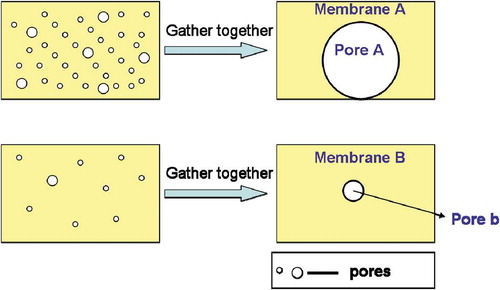
For the dynamic model in this study, it is assumed that the high water flux of the GO film is caused by the microstructure of GO, including its valleys, folds, cavitations and voids. We first prepare two support membranes: membrane A and membrane B. It is assumed that membrane A and membrane B have the same structures (individual pore size, hydrophilicity, roughness, thickness, etc.) except for the number of pores on the membrane surface. Thus, the membrane water flux is only determined by the number of surface pores. The more pores there are on the surface, the higher the water flux is. Thus, membrane A, which has a greater number of pores, has a higher flux, while membrane B has a lower water flux. In this study, it is assumed that all pores can be collected and assembled into a single large pore, as described in Figure 1. In this case, the assembled pore of membrane A is larger than that of membrane B.

Figure 1. Schematic of the support membranes with high flux (A) and low flux (B).

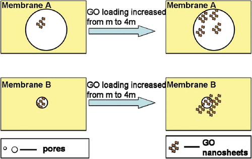
For the layered GO membrane, GO loading can affect the water flux of the composite membrane. If the initial GO loading is assumed to be m, then the pores on membrane A are assumed to be approximately 10% covered, and the smaller number of pores on membrane B will be approximately 70% covered. When GO loading is increased from m to 4m, the coverage of the pores on membrane A will increase to approximately 40%, and the coverage of the pores on membrane B will increase to approximately 80%, as shown in Figure 2. Correspondingly, the change in the flux of water through membrane A increases from a 10% to a 40% reduction and that of membrane B increases from a 70% to an 80% reduction. Therefore, we can conclude that the effect of GO loading on the flux of the composite membrane is related to the initial water flux of the composite membrane. Moreover, GO loading has a larger effect on a composite membrane with a larger flux and little effect on a composite membrane with a smaller flux.

Figure 2. The effect of GO loading on the surface pores of the hybrid membranes.

The membrane flux is represented by Q, and the GO loading is represented by m. With a change in GO loading (Δm), the membrane flux of water will also change (ΔQ). The change in water flux (ΔQ) is related to the initial membrane water flux (Q). Thus, formula (2) can be obtained in this study:

(2) $-\frac{dQ}{dm}=kQ$(2)

where k is the change coefficient of the membrane flux. Equation (2) can be rewritten as formula (3)

(3) $-\frac{dQ}{Q}=kdm$(3)

Then, formula (4) can be obtained by integrating both sides. Formulas (4), (5) and (6) can be obtained by integration. By solving the equation, Equation (7) for the membrane flux can be obtained.

(4) $-\int \frac{dQ}{Q}=\int kdm$(4)

(5) $-lnQ=km+a_1$(5)

(6) $lnQ=-a_1-km=a_2-km$(6)

(7) $Q=e^{a_2-km}=e^{a_2}\cdot e^{-km}=a\cdot e^{-km}$(7)

where k, a₁, a₂ and a are constants.

The k is the change rate of the membrane flux onto per mass of oxidized graphene. The m is the pre-exponential factor, which depends on the inner reaction properties and independent of the temperatures and the concentrations.

When m is equal to 0, e^−km is equal to 1 and $Q=Q_{max}$

As m approaches infinity, e^−km approaches 0 and $Q=Q_{min}$approaches 0.

3.2 Verification of the water transfer dynamics equation in the BPPO/GO composite membrane

Figure 3 shows the effect of GO loading on the water flux of the prepared BPPO/GO membrane. As shown in Figure 3, with increasing GO loading from 0 mg/m² to 39 mg/m², the BPPO/GO membrane flux decreases linearly from 550 L/m²·h·bar to 44.89 L/m²·h·bar. Further increasing the GO loading from 39 mg/m² to 78 mg/m² reverses the reduction of the BPPO/GO membrane flux. The results show that the water flux is related to the loading of GO. The higher the GO loading is, the thicker the formed GO membrane, and the higher the resistance to water transport.

Figure 3. Effect of GO loading on water flux of the prepared BPPO/GO membranes.

Combining the experimental results in Figure 3 and dynamics Equation (7), the simulated results are obtained and shown in Figure 4. The blue markers are the experimental values of the water flux, and the red curve is the simulated results.

Figure 4. Simulation results based on experimental results. (The MATLAB calculation code is shown in Appendix A).

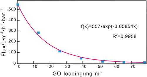
The simulation results (Figure 4) show that a = 557, k = −0.05854 and the water transport dynamics equation in the BPPO/GO composite membrane in this study can be expressed as:

$Q=557\cdot e^{-0.05854m}$

The obtained equation was analyzed by regression analysis, and the results are shown in Tables 1, 2 and 3.

Table 1. The regression analysis of the BPPO/GO membrane experimental results.

Multiple R	R squared	Adjusted R squared	Standard error	Observation value
0.9982	0.9964	0.9957	13.0458	7

Table 2. The variance analysis of the BPPO/GO membrane experimental results.

Variance analysis	df	SS	MS	F	Significance of F
Regression Analysis	1	241,402.8077	241,402.8077	1418.4020	2.49E-07
Residual Error	5	850.9675	170.1935
Total	6	242,253.7752

Table 3. The regression parameters of the BPPO/GO membrane results.

	Coefficients	Standard error	p-Value	Lower limit 95.0%	Upper limit 95.0%
Intercept	6.7726	6.2046	0.3248	−9.1770	22.7222
X Variable 1	0.9800	0.0260	2.49E-07	0.9131	1.0469

The degree of freedom is equal to the number of samples minus the number of variables minus 1; here, the degree of freedom is 5. For a significance level of 0.05, the correlation coefficient for the critical value of a test is 0.75994. In this study, the correlation coefficient is 0.9982 > 0.75449, suggesting that the regression analysis is significant.

When p < 0.05, we can consider the model to be significant at α = 0.05, or the confidence level is 95%; when p < 0.01, we can consider the model to be significant at α = 0.01, or the confidence level is 99%; when p < 0.001, we can consider the model to be significant at α = 0.001, or the confidence level is 99.9%. For the model in this study, p = 0.0000000542 < 0.0001, and we can consider the model to be significant at α = 0.0001, or the confidence level is 99.99%. From the above fitting results, we confirm that the dynamic model is consistent with the experimental results, which proves the validity of the dynamic equation.

3.3 Verification of the water transport dynamics equation with previous scientific research

3.3.1 Application of the developed dynamic equation to the results of huang et al

To further verify the validity and applicability of the dynamics equation developed in this study, the dynamics equations were applied to fit the results of previously reported research. Han et al. [14]. fabricated an ultrathin layered GO membrane by filtering an extremely dilute solution of base-refluxed reduced GO (brGO) through a microporous substrate. The prepared ultrathin graphene nanofiltration membranes (uGNMs) showed well-packed layered structures. Figure 5 shows that the uGNMs that had the lowest loading of brGO (14.1 mg/m²) exhibited the highest water permeability (21.8 L/m2·h·bar). With increased brGO loading, the water flux decreased from 21.81 to 3.26 L/m2·h·bar. Figure 6 shows the results of the reported experimental results fit by the developed dynamics equations. The blue markers are the experimental values of the water flux, and the red curve is the simulated results. (The MATLAB calculation code is shown in Appendix B).

Figure 5. Variation in the pure water flux as a function of the brGO loading of the membranes [14].

Figure 6. Simulated results based on Han’s experiment results.

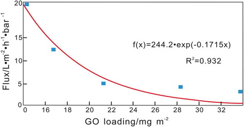
From the fitting result in Figure 6, the constant a is calculated to be 244.2, while the constant k is −0.1715. Therefore, the transfer kinetics equation of the water flux through the composite membrane is:

$Q=244.2\cdot e^{-0.1715m}$

The obtained equation was further analyzed by regression analysis, and the results are shown in Table 4 and the Support Information (Table S1 and Table S2).

Table 4. The regression analysis of the experimental results of Han et al.

Multiple R	R squared	Adjusted R squared	Standard error	Observation value
0.9760	0.9527	0.9369	2.1847	5

For a degree of freedom of 3 and a significance level of 0.05, the correlation coefficient for the critical value of a test is 0.87834, which can be obtained from a mathematical table. In this study, the correlation coefficient is 0.9760, which is larger than 0.87834, indicating that the regression analysis is significant.

When p < 0.05, we can consider the model to be significant at α = 0.05, or the confidence level is 95%; when p < 0.01, we can consider the model to be significant at α = 0.01, or the confidence level is 99%; when p < 0.001, we can consider the model to be significant at α = 0.001, or the confidence level is 99.9%. For the results of Han et al., p = 0.0000000542 < 0.0001, and we can consider the model to be significant at α = 0.0001, or the confidence level reaches 99.99%. From the above fitting result, we can conclude that the dynamic model is consistent with the experimental results. Additionally, the developed dynamics equation is proven to be applicable to the research results of Han et al.

3.3.2 Application of the developed dynamic equation to the results of huang et al

Huang et al. reported nanostrand-channeled graphene oxide ultrafiltration membranes, which contained a network of nanochannels with a narrow size distribution (3–5 nm) and exhibited superior separation performance [27]. The layered GO membrane was prepared by filtering a mixed solution of GO and copper hydroxide nanostrands (CHNs) through a PC membrane, which was followed by hydrazine reduction and CHN removal. The dynamics equation developed in this study were used to simulate the results of Huang et al. (Figure 7). Figure 8 shows the results of fitting the data of Huang et al. with the kinetics equation developed in this study. The blue markers are the experimental values for the water flux, and the red curve is the simulated results. (The MATLAB calculation code is shown in Appendix C).

Figure 7. Thickness-dependent separation performance of the graphene oxide membranes.

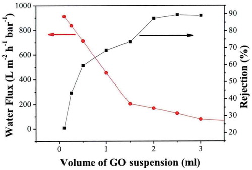
Figure 8. Simulated results based on the experimental results of Huang et al.

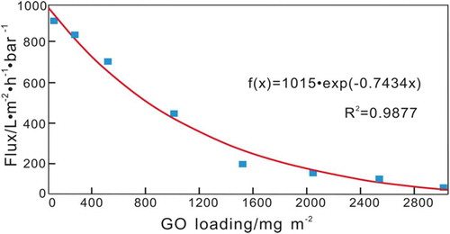
According to the above fitting results, a is equal to 1015, and k is equal to −0.7434. The obtained transfer kinetics equation of the water flux through the composite membrane is:

$Q=1015\cdot e^{-0.7434m}$

The obtained equation was analyzed by regression analysis, and the results are shown in Table 5 and Support Information Tables S3 and S4.

Table 5. The regression analysis of the experimental results of Huang et al.

Multiple R	R squared	Adjusted R squared	Standard error	Observation value
0.9933	0.9868	0.9841	35.9466	7

For a degree of freedom of 5 and a significance level of 0.05, the correlation coefficient for the critical value of a test is 0.75449. In this study, the correlation coefficient for these experimental values is 0.9933 > 0.75449. It can be seen that the results of the regression analysis are significant.

For this example, p = 6.79E-06 < 0.0001. Therefore, the results can be considered at the α = 0.0001 level of significance, or the confidence coefficient is 99.99%. The above fitting results show that the developed dynamics model is in good agreement with the experimental results. It can be seen that the developed dynamics equation is also applicable to the research results of Huang et al.

In summary, the transfer dynamics equation developed in this study for the water flux through a BPPO/GO composite membrane is in good agreement with the experimental results. The kinetics equation is also suitable for previously reported layered GO membranes.

4. Conclusions

A water transport kinetics model for layered GO membranes was developed, and the kinetic equation is in good agreement with our experimental results. At the same time, the results of previously reported layered GO membranes were fit with the kinetics equation developed by us. The fitting results were highly consistent, which showed that the dynamics equation developed in this study is widely applicable. This theoretical kinetic study provides insight into the application of graphene oxide membranes in water treatment.

Acknowledgments

The authors gratefully acknowledge the financial support of the Natural Science Foundation of Jiangsu Province (Grant No. BK20170249) and the Natural Science Fund for Colleges and Universities of Jiangsu Province (Grant No. 17KJB610012, Grant No. 18KJA610003). We also thank Prof. Xiwang Zhang (Department of Chemical Engineering, Monash University) for helping to improve the manuscript. Xueyang Zhang especially thanks the Science and Technology Plan Projects of Xuzhou City (Grant No. KC18150).

Disclosure statement

No potential conflict of interest was reported by the authors.

Additional information

Funding

This work was supported by the the Natural Science Foundation of Jiangsu Province [BK20170249];the Science and Technology Plan Projects of Xuzhou City [KC18150];the Natural Science Fund for Colleges and Universities of Jiangsu Province [17KJB610012, 18KJA610003].

Appendix A

x = [0 13,25 39 52 65 78];

y = [550 284 112 44.89 15 4.1 3.14];

cftool


General model Exp1:

  f(x) = a*exp(b*x)

Coefficients (with 95% confidence bounds):

   a = 557 (520.6, 593.5)

   b = −0.05854 (−0.06619, −0.0509)


Goodness of fit:

 SSE: 1057

 R-square: 0.9958

 Adjusted R-square: 0.995

 RMSE: 14.54

Appendix B

x = [14.2 16.72 21.3 28.3 33.8];

y = [22.36 12.5 5.06 4.46 3.3];

cftool


General model Exp1:

  f(x) = a*exp(b*x)

Coefficients (with 95% confidence bounds):

   a = 244.2 (−273.5, 761.9)

   b = −0.1715 (−0.3078, −0.0351)


Goodness of fit:

 SSE: 17.54

 R-square: 0.932

 Adjusted R-square: 0.9093

 RMSE: 2.418

Appendix C

x = [0.1 0.289402 0.58663 1.180243 1.77847 2.391629 2.979258 3.56];

y = [830.3896 706.1038 446.0721 200.2775 162.6748 124.5869 80];

cftool


General model Exp1:

  f(x) = a*exp(b*x)

Coefficients (with 95% confidence bounds):

   a = 1015 (926.9, 1102)

   b = −0.7434 (−0.8718, −0.615)


Goodness of fit:

 SSE: 9864

 R-square: 0.9877

 Adjusted R-square: 0.9857

 RMSE: 40.55

References

- Dreyer DR, Park S, Bielawski CW, et al. The chemistry of graphene oxide. Chem Soc Rev. 2010;39(1):228–240.
- Guan K, Shen J, Liu G, et al. Spray-evaporation assembled graphene oxide membranes for selective hydrogen transport. Sep Purif Technol. 2017;174:126–135.
- Safarpour M, Vatanpour V, Khataee A, et al. Development of a novel high flux and fouling-resistant thin film composite nanofiltration membrane by embedding reduced graphene oxide/TiO 2. Sep Purif Technol. 2015;154:96–107.
- Song JJ, Huang Y, Nam S-W, et al. Ultrathin graphene oxide membranes for the removal of humic acid. Sep Purif Technol. 2015;144:162–167.
- Zhu J, Meng X, Zhao J, et al. Facile hydrogen/nitrogen separation through graphene oxide membranes supported on YSZ ceramic hollow fibers. J Membr Sci. 2017;535:143–150.
- Meng N, Priestley RCE, Zhang Y, et al. The effect of reduction degree of GO nanosheets on microstructure and performance of PVDF/GO hybrid membranes. J Membr Sci. 2016;501:169–178.
- Meng N, Wang Z, Low Z-X, et al. Impact of trace graphene oxide in coagulation bath on morphology and performance of polysulfone ultrafiltration membrane. Sep Purif Technol. 2015;147:364–371.
- Zeng X, Wang Z, Meng N, et al. Highly dispersed TiO 2 nanocrystals and carbon dots on reduced graphene oxide: ternary nanocomposites for accelerated photocatalytic water disinfection. Appl Catal B. 2017;202:33–41.
- Golpour M, Pakizeh M. Development of a new nanofiltration membrane for removal of kinetic hydrate inhibitor from water. Sep Purif Technol. 2017;183:237–248.
- Hwang T, JoonSuk, Yim, et al. Ultrafiltration using graphene oxide surface-embedded polysulfone membranes. Sep Purif Technol. 2016;166:41–47.
- Ko K, Yu YJ, Kim MJ, et al. Improvement in fouling resistance of silver-graphene oxide coated polyvinylidene fluoride membrane prepared by pressurized filtration. Separation & Purification Technology; 2018;194:161–169.
- Liu Z, Wu W, Liu Y, et al. A mussel inspired highly stable graphene oxide membrane for efficient oil-in-water emulsions separation. Sep Purif Technol. 2018;199:37–46.
- Xu HM, Sun XF, Wang SY, et al. Development of laccase/graphene oxide membrane for enhanced synthetic dyes separation and degradation. Sep Purif Technol. 2018;204: 255–260.
- Han Y, Xu Z, Gao C. Ultrathin graphene nanofiltration membrane for water purification. Adv Funct Mater. 2013;23(29):3693–3700.
- Huang H, Song Z, Wei N, et al. Ultrafast viscous water flow through nanostrand-channelled graphene oxide membranes. Nat Commun. 2013;4(4):2979.
- Choi W, Choi J, Bang J, et al. Layer-by-layer assembly of graphene oxide nanosheets on polyamide membranes for durable reverse-osmosis applications. Acs Appl Mater Interfaces. 2013;5(23):12510–12519.
- Hu M, Mi B. Layer-by-layer assembly of graphene oxide membranes via electrostatic interaction. J Membr Sci. 2014;469(11):80–87.
- Liu G, Jin W, Xu N. Graphene-based membranes. Chem Soc Rev. 2015;44(15):5016–5030.
- Kim HW, Yoon HW, Yoon S-M, et al. Selective gas transport through few-layered graphene and graphene oxide membranes. Science. 2013;342(6154):91–95.
- Jilani A, Othman MHD, Ansari MO, et al. A simple route to layer-by-layer assembled few layered graphene oxide nanosheets: optical, dielectric and antibacterial aspects. J Mol Liq. 2018.
- Borges DD, Woellner CF, Autreto PAS, et al. Insights on the mechanism of water-alcohol separation in multilayer graphene oxide membranes: entropic versus enthalpic factors. Carbon. 2018;127:280–286.
- Chen B, Jiang H, Liu X, et al. Molecular insight into water desalination across multilayer graphene oxide membranes. ACS Appl Mater Interfaces. 2017;9(27):22826–22836.
- Huang H, Song Z, Wei N, et al. Ultrafast viscous water flow through nanostrand-channelled graphene oxide membranes. Nat Commun. 2013;4:2979.
- Borges DD, Woellner CF, Autreto PAS, et al., Insights on the mechanism of water-alcohol separation in multilayer graphene oxide membranes: entropic versus enthalpic factors. 2017.
- Chen B, Jiang H, Liu X, et al. Molecular insight into water desalination across multilayer graphene oxide membranes. Acs Appl Mater Interfaces. 2017;9(27):22826.
- Meng N, Zhao W, Shamsaei E, et al. A low-pressure GO nanofiltration membrane crosslinked via Ethylenediamine. J Membr Sci. 2017.
- Huang H, Song Z, Wei N, et al. Ultrafast viscous water flow through nanostrand-channelled graphene oxide membranes. Nat Commun. 2012;4(4):345–350.