Computational welding simulation of a plasma wire arc additive manufacturing process for high-strength steel

Abstract

Wire arc additive manufacturing (WAAM) processes have many advantages including the ability to repair worn or damaged components. Compared to other arc processes, plasma welding constricts the arc, which leads to a highly concentrated energy input. Thus, an understanding of the heat input distribution and its consequences such as transient temperature field, transformation, build up of stresses, and distortion is of great importance for applications with high-strength steels. Numerical simulation can provide an important input for this evaluation. However, the plasma arc is challenging to simulate due to its high energy density and thus steep gradients, as standardly used heat sources in commercial software often only represent classical arc or beam processes. Therefore, this study deals with the development of an accurate heat source model based on standard implemented heat sources in Simufact Welding. Therefore, welding experiments were performed on steel and thermal cycles representing the quasi-­stationary temperature field were recorded. Subsequently, metallographic examinations were performed describing the fusion and heat-affected zone. On this basis, distortion simulations were carried out and validated using further welding experiments. Using the obtained results, path planning, idle time, and consequently interpass temperatures and the resulting heat flow can be analysed.

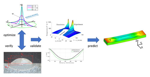
Graphical Abstract

Keywords:

• Simulation
• high strength steel
• plasma arc

1. Introduction

The field of additive manufacturing (AM) processes is new compared to conventional manufacturing processes. In the last decades, a lot of research and development has been done and great progress has been made, which enabled AM to enter the industry. Based on a CAD geometry, ready-to-use components can be manufactured quickly and easily. The material is deposited layer by layer, each layer corresponding to a thin cross-section profile of the 3D geometry. The thinner the layers, the more accurate the components (Gibson, Rosen, & Stucker, 2014). In general, a heat source (arc, laser, or electron beam) is used to liquefy metal powder or wire to deposit it in layers (Michaleris, 2014). The wire arc additive manufacturing (WAAM) process is ideally suited for the fabrication of large components made of various metallic materials. The advantages over powder-based systems are the high build rate, the low material costs, and good availability over a wide range of different materials and the resulting good structural integrity of the final part. The process, which belongs to the group of direct energy deposition (DED) processes, typically uses an electric arc as a heat source to melt a metallic wire. Commercially available welding processes are commonly used as welding heat sources. The movement of the welding torch is controlled by robotic systems or CNC machines (Williams et al., 2016).

If a plasma welding is used as heat source the process is designated as plasma wire arc additive manufacturing (PWAAM). The plasma welding process is similar to the TIG process as it uses a non-melting tungsten electrode to generate the arc. The main difference between the two processes is the constricting the arc using a specially designed nozzle and a plasma gas, which leads to an increase in energy density and the stability of the arc at the same current. In the process, the plasma reaches temperatures of up to 25,000 °C (Sahoo & Tripathy, 2021).

Numerical simulations can be carried out to gain a deeper understanding of the WAAM process in terms of the temperature fields, deformation, and residual stresses (Casuso et al., 2021). From a simulation point of view, WAAM processes are very similar to multipass welding processes. The simplified physical model of the complex heat and mass transfer enables the calculation with acceptable computation times. A transient coupled thermomechanical finite element analysis is most commonly used, where a heat source model describes introduced energy. The progressive material deposition is achieved with specific element activation procedures (Montevecchi, Venturini, Scippa, & Campatelli, 2016). Residual stresses and distortion are the consequence of the resulting temperature field caused by the heat input required to create the melt pool. Due to the good thermal conductivity of metallic materials, a high heat concentration is necessary. Temperature and phase-dependent thermal expansion and phase transformation are the most important material properties governing residual stresses build up (Radaj, 2013). The finite element method (FEM) can be used to investigate residual stresses and distortions in advance, thus, optimizing path planning and avoiding trial and error iterations (Denlinger & Michaleris, 2016).

This study is dealing with the development of a simulation model which describes the PWAAM process for high strength steel. The FE-software Simufact Welding is used for the analysis. Good agreement between the simulated and experimental obtained temperature fields and distortion is the main objective of this investigation which is experimentally verified.

2. Method

2.1. Finite element model

The nonlinear FE-calculation was carried out with the software Simufact Welding. The model shown in Figure 1 was created and represents the experimental process. It was used to calibrate the heat source model. The dimensions of the substrate are 175 mm × 40 mm × 30 mm. The weld bead dimensions are 1.2 mm in height, 7.9 mm in width, and 150 mm in length and were obtained from the experiment. The bearings represent the mechanical support used in the experiment.

Figure 1. FE-Model for heat source calibration.

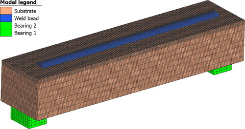
The required mesh size for the 8-node brick elements was obtained by executing a mesh convergence study. For a good resolution of the steep temperature gradients the mesh size of the weld bead and in the surface area of the substrate is set to 0.5 mm. In total, the model contains of 373.000 brick elements and 410.000 nodes.

2.2. Material model

The used base material in this study is a modified C55 steel and the used filler material is a low alloyed filler wire from the Company BÖHLER with the name 3Dprint AM 80 HD. Table 1 shows the chemical composition of the used materials. The material parameters required for the simulation model were not available in the Simufact Welding database. They were calculated with the software JMatPro. Thus, the temperature-dependent values for the thermal conductivity, elastic modulus, specific heat capacity, Poisson’s ratio, density, and coefficient of thermal expansion were calculated up to 1600 °C and implemented in the Simufact Welding material model.

Table 1. Chemical composition in mass% of modified C55 (EN ISO 683-1, 2018) and 3Dprint AM 80 HD (Voestalpine Böhler Welding Austria GmbH, 2023) nominal according to datasheet.

	C	Si	Mn	P	S	Cr	Cu	Mo	Ni	V
Modified C55	0.56	0.40	0.80	0.02	0.015	0.30	0.30	0.08	0.30	0.06
3Dprint AM 80 HD	0.09	0.40	1.70	–	–	0.35	–	0.60	2.00	–

2.3. Heat source model

Proper modeling of the transient heat source is fundamental for the simulation of welding and AM processes. The aim is to precisely reproduce the amount of heat introduced by the plasma arc and its distribution. In the used software Simufact Welding, it is possible to distinguish between double elliptic Goldak heat source model, Gaussian surface heat source model or conical heat source model. In this study, the conical heat source model will not be considered further. (1) $$q_f\left(x,y,z,t\right)=\frac{6\sqrt{3}{f}_{f}Q}{a_f\mathit{\text{bd}}\pi \sqrt{\pi }}\mathrm{e}\mathrm{\text{xp}}\left[-\frac{M{\left(x-v_{s}t\right)}^2}{a_f^2}-\frac{M{y}^2}{b^2}-\frac{M{z}^2}{d^2}\right]$$(1) (2) $$q_r\left(x,y,z,t\right)=\frac{6\sqrt{3}{f}_{r}Q}{a_f\mathit{\text{bd}}\pi \sqrt{\pi }}\mathrm{e}\mathrm{\text{xp}}\left[-\frac{M{\left(x-v_{s}t\right)}^2}{a_r^2}-\frac{M{y}^2}{b^2}-\frac{M{z}^2}{d^2}\right]$$(2)

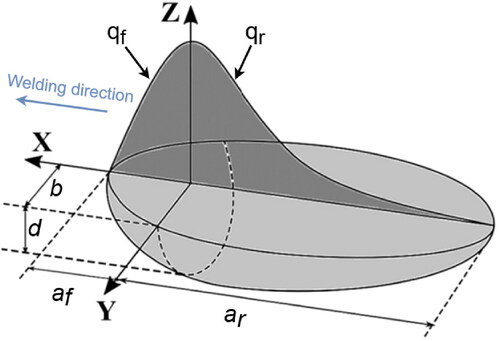
The double elliptical heat source model which is shown in Figure 2 is the most used heat source in welding simulation as arc welding processes can be described properly. It was developed specifically for welding simulation by Goldak et al. (Goldak, Chakravarti, & Bibby, 1984). The heat source model thereby describes the Gaussian distribution of the introduced heat per unit volume, which is defined in a moving reference frame. A Cartesian coordinate system with origin in the welding center is introduced. The x-axis points in the welding direction, the z-axis points in the direction of the sheet thickness, and the y-axis is perpendicular to the welding direction. The heat source moves with a constant welding speed $v_s$[m/s] along the x-axis. The power distribution functions $q_f$ and $q_r$[W/m³] define the introduced heat in the front and behind of the semi-axis, which allows the modeling of an asymmetric heat distribution along the x-axis. $a_f$[m] is the front length, $a_r$ [m] is the rear length, b [m] is the width, and d [m] is the depth of the ellipsoid volume in which the total arc power Q [W] is distributed. The parameters ${ f}_f$ and ${ f}_r$ define the fraction of heat in the front and back parts of the ellipsoid, satisfying the condition ${ f}_f$ + ${ f}_r$ = 2. (3) $$q_s\left(x,y,t\right)=\frac{3Q}{\pi r_s^2}\mathrm{e}\mathrm{\text{xp}}\left[-\frac{M{\left(x-v_{s}t\right)}^2}{r_s^2}-\frac{M{y}^2}{r_s^2}\right]$$(3)

Figure 2. Double elliptical Goldak heat source model (Rubio-Ramirez, Giarollo, Mazzaferro, & Mazzaferro, 2021).

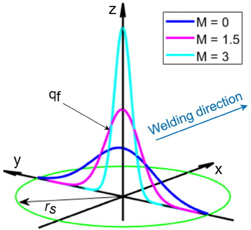
The Gaussian surface heat source model was developed before the double elliptical heat source model of Pavelic (1969). Here, the heat input is described by a Gaussian distribution on the surface. This surface heat source can be used for modeling beam welding processes but can also be used for arc welding processes as well (Mayer, 2023). The power distribution functions $q_s$ [W/m²] thereby distributes the applied power Q symmetrically about the z-axis onto the surface, moving with velocity $v_s$ along the x-axis. The parameter $r_s$ [m] is the radius of the circle which is affected by the heat source and M gives the Gaussian parameter defining the geometry of the Gaussian bell curve. Three power distribution functions with different values for the parameter M are shown in Figure 3.

Figure 3. Gaussian heat source model.

3. Experiment

To calibrate and evaluate a heat source, conducting an experiment is essential. In this study, this was done with the machine M3DP-SL from the company SBI GmbH. This power source enables a PWAAM process and is used for research purposes in the field of AM. In the experiment, a 150 mm long weld was deposited on the modified C55 plate. The already mentioned filler wire 3Dprint AM 80 HD with a diameter of 1.2 mm was used. It is fed against the welding direction into the plasma (Mayer, 2023). A plasma nozzle with a diameter of 5 mm was used. To measure the temperature distribution, six thermocouples were placed 7 mm, 9 mm, 11 mm, 14 mm, 18 mm, and 24 mm away from the weld line center. A type S thermocouple was used at the closest position while type K thermocouples were used at the other five positions. Finally, all thermocouples were covered with ceramic tubes and water glass to protect them from the thermal radiation generated by the plasma arc.

The used welding parameter for the experiment are shown in Table 2 where I [A] is the welding current, U [V] the welding voltage, $v_s$ [mm/s] the welding speed, $v_D$ [mm/s] the wire feed speed, $\dot{{ V}_s}$ [l/min] the shielding gas flow rate, and $\dot{{ V}_P}$ [l/min] the plasma gas flow rate. The voltage U adjusts itself according to the power source characteristic and was, therefore,, not specified. The voltage was measured during the welding process and was subsequently given as an averaged value in the simulation model.

Table 2. Welding parameters for experiment.

I [A]	U [V]	$v_s$ [mm/s]	$v_D$ [mm/s]	$\dot{{ V}_s}$ [l/min]	$\dot{{ V}_P}$ [l/min]
260	22.4	4	48	15	1.5

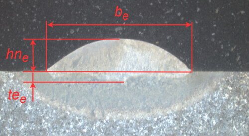
During the welding process, the temperature was recorded with a 50 Hz sample rate. After the welding was done, the sample was cut transvers to the weld to create a cross-sectional micrograph of the weld (Figure 4). The parameters ${\mathit{\text{te}}}_e$ [mm], ${\mathit{\text{hn}}}_e$ [mm] and $b_e$ [mm] determine the penetration depth, weld height and weld width. The index e indicates the experiment.

Figure 4. Cross-sectional micrograph transvers to weld seam.

To evaluate the accuracy of the thermomechanical simulation model, a distortion experiment was performed additionally. A specimen geometry of 25 mm × 130 mm × 8 mm was used to increase the warpage. To minimize initial residual stresses, the specimens were normalized at 860 °C for 25 min. The cooling was done in the oven, with still air. A 100 mm long weld was deposited on the specimen using the welding parameters from Table 2. After cooling of the specimen to ambient temperature, the distortion of the sample was measured on the backside of the specimen.

4. Heat source calibration

With the experimentally determined thermal cycles and weld pool dimension the heat source model can be calibrated. The temperature field as well as the shape of the melt pool, which is simulated, must be in good agreement with the experimentally recorded measured values. The parameters described in model of Figure 1 are used to calibrate the heat source model. In the simulation, a time increment size of 0.1 s is used. Using the trial-and-error method, the input parameters of the heat source are varied until the geometry of the molten volume agree with the experiment. A total of 27 simulations were performed to calibrate the heat source. To quantitatively evaluate the deviation of experimental and numerically modelled weld pool geometry, the relative errors are calculated as follows: (4) $$b_v=\left(\frac{b_s}{b_e}-1\right)\hspace{0.17em}\hspace{0.17em}\text{*}100$$(4) (5) $$t{e}_v=\left(\frac{t{e}_s}{t{e}_e}-1\right)\hspace{0.17em}\hspace{0.17em}\text{*}100$$(5) (6) $$A{u}_v=\left(\frac{A{u}_s}{A{u}_e}-1\right)\hspace{0.17em}\hspace{0.17em}\text{*}100$$(6) (7) $$A=\frac{\mathit{\text{Au}}}{\mathit{\text{Ag}}}$$(7) (8) $$A_v=\left(\frac{A_s}{A_e}-1\right)\text{*}100$$(8) where $b_v$ [%] is the width ratio, $t{e}_v$ [%] the penetration depth ratio, $A{u}_v$ [%] the ratio of the lower melt pool areas ${\mathit{\text{Au}}}_s$[mm²] and ${\mathit{\text{Au}}}_e$ [mm²]. The dilution $A$ [%] is defined in Eq. (7)(7) $$A=\frac{\mathit{\text{Au}}}{\mathit{\text{Ag}}}$$(7) where $A_g$ [mm²] is the total melt pool area. $A_v$ [%] is the dilution ratio of simulated to experimentally recorded melt pool geometry. Index s stands for simulation result. If the value is negative, it indicates that the simulation value is smaller than that of the experiment. If the value is positive, the simulation value is larger than the experimentally measured one. To give a better overview of the results of the simulations performed, the simulation results ${\mathrm{b}}_{\mathrm{v}}$, $t{e}_v$, $A{u}_v$, and $A_v$ are shown over the simulation number in Figures 5 and 6. 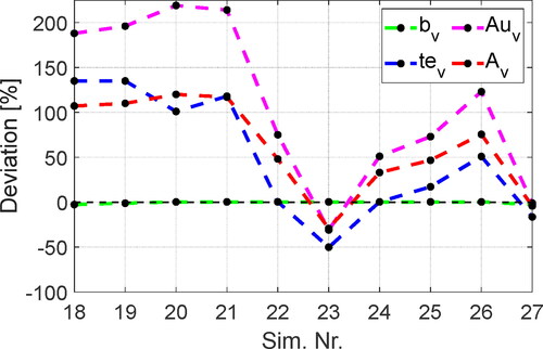The width ratio ${\mathrm{b}}_{\mathrm{v}}$ is very close to 0% at all performed simulations. When the double elliptical heat source is used (Figure 5), the results deviate strongly from the experimentally determined sizes. By using the Gaussian surface heat source, better agreement with the experiment is obtained when considering the melt pool geometry than with the double elliptical heat source. In addition to the melt pool geometry, the simulated temperature distribution must match the experimentally determined one.

Figure 5. Deviation of the simulation from the experimentally determined melt pool geometry (double elliptical heat source).

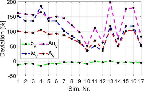
Figure 6. Deviation of the simulation from the experimentally determined melt pool geometry (Gaussian heat source).

The temperature curves of simulation no. 27 are shown in Figure 7 together with those determined experimentally. The measured values of the thermocouple $T{e3}_e$ are not considered due to a measurement error. It is visible that the five temperature curves measured at different distances from the weld line are in good agreement with each other. The values of the $t_{8/5 }$ time of the simulation and of the experiment are also in the same order of magnitude. After 180 s, the measured and simulated temperature gradients asymptotically reach a common final temperature. The resulting temperature is independent of the dimensions of the heat source model but depends only on the amount of energy introduced and the thermal mass of the geometry. Which means that the correct thermal efficiency η was used in the simulation model (Rissaki, 2022). The melt pool geometry and the temperature curves of the simulation match the results of the experiment well, which is why the validated heat source is later used for the thermomechanical simulation. Table 3 shows the parameters of the calibrated Gaussian heat source.

Figure 7. Temperature profiles simulation no. 27 and experiment.

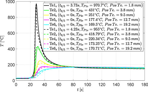
Table 3. Heat source parameters.

voltage U [V]	22.4
current I [A]	260
welding speed $v_s$ [mm/s]	4
efficiency η [%]	55
circle radius $r_s$ [mm]	8
Gaussian parameter M [-]	1.5

5. Results

5.1. 3D temperature field

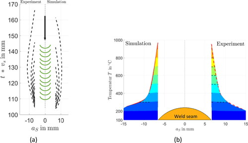
With the temperature curves of the simulation and the experiment a three-dimensional temperature field can be generated, using the software, MATLAB. With fit functions, a thermal body visualizes the temperature distribution on the sheet surface based on the calculated thermal field. The 3D temperature fields shown in Figure 8 represents the temperature distribution next to the weld and is generated with the measured temperature curves and the position of the thermocouples. The temperature field of the experiment is compared with the simulation results. Additionally, results can be derived from a two-dimensional view. The top view of the thermal body shows the isotherms on the surface of the substrate (Figure 9(a)), with the black arrow pointing in the welding direction. The dashed black lines represent the isotherms, plotted in steps of 100 °C. It can be seen that the length as well as the width of the lines of the simulation are in good agreement with those of the experiment. The two-dimensional view of the 3D temperature fields in welding direction is visualized in Figure 9(b) and shows the temperature distribution on the substrate surface transverse to the weld.

Figure 8. 3D temperature field validated heat source.

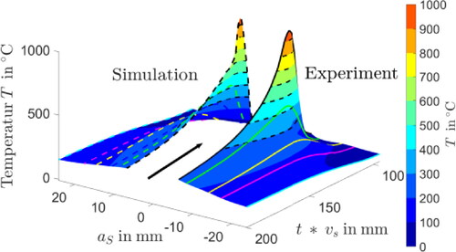
Figure 9. (a) Isothermal temperature field, (b) transverse temperature distribution.

5.2. Distortion simulation

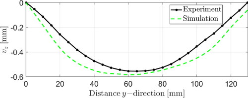
The aim of the thermomechanical simulation was to make a prediction about the resulting distortion. The thermomechanical simulation model uses the geometry, materials, and welding parameters of the experiment described in chapter 3. The validated Gaussian surface heat source is used as a thermal boundary condition Figure 10. The one-sided heat input leads to distortion of the sample. Due to the selected geometry, the specimen warps strongly around one main axis of inertia (x-direction) leading to massive deformation in z-direction. In x- and y-direction only a minimal deformation occurs. The distortion $v_z$ measured on the backside of the specimen is shown in Figure 11 along the welding seem position (y-distance). The simulation results are in good agreement with the experimentally measured distortion, with a maximum deviation of 0.11 mm (30%). The simulation model with the validated heat source gives acceptable results when calculating the warpage.

Figure 10. Surface deviation 4 times magnified.

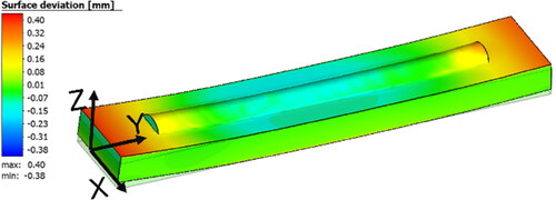
Figure 11. Comparison of distortion on sample backside.

6. Conclusion

The goal of this study was to generate an accurate representation of the plasma process with one of the standard implemented heat sources to use for temperature and distortion predictions. This was done with a detailed evaluation of the process and the trial-and-error method. This method was very time-consuming due to the large number of independent heat source parameters and fine mesh, as many simulations had to be carried out. Nevertheless, it was possible to create an accurate heat source for the plasma arc which brings good results for thermal and distortion analysis. When considering the melt pool geometry of the experiment, it can be noted that the penetration depth ${\mathit{\text{te}}}_e$ is much smaller than the height of the weld ${\mathit{\text{hn}}}_e$. This low penetration depth and its flat shape is untypical for classical arc processes and shows the challenge of the plasma arc.

• With the double elliptical heat source, it was not possible to model the experimentally determined melt pool geometry properly, while at the same time matching the temperature profiles.

• Using the 2D Gaussian surface heat source, a good agreement of the melt pool geometry and the temperature profiles could be achieved.

The advantage of the Gaussian surface heat source in comparison to the double elliptical heat source is the small quantity of independent simulation parameters, which simplifies the adjustment of the heat source using the trial-and-error method.

Although the Gaussian heat source is usually preferred for beam processes, it can represent the plasma process better. This was achieved in the concrete case as follows:

• The source acts only on the surface of the substrate.

• A lower Gaussian parameter which leads to a flatter energy distribution in combination with an increased cross-sectional radius of the heat source.

This study shows the possibility of demonstrating the plasma arc with common heat sources but also the effort behind it. Since the plasma arc can be strongly changed by the nozzle cross section and the amount of plasma gas, it is obvious to develop a new heat source model for plasma welding process. This could function as a link between the Gaussian and Goldak model.

6.1. Outlook

The heat source developed in this study can now subsequently be used to make predictions about local temperature cycles in the Material. This is particularly important for the used base material, with its high C content. The resulting deformation can also be considered for planned parts. These aspects can be incorporated into the path planning of the PWAAM process in the future. Improvements to the model itself are also being worked on, as the current heat source only covers a certain set of process parameters. The creation and evaluation of such a heat source should be simplified to make the process more flexible. Here, the approach of a separate heat source for the PWAAM is also of interest.

Disclosure statement

No potential conflict of interest was reported by the authors.

Additional information

Funding

We would like to thank the Federal Ministry for Climate Protection, Environment, Energy, Mobility, Innovation and Technology (BMK), the Federal Ministry of Labor and Economic Affairs (BMAW), the Austrian Research Promotion Agency (FFG) and the four provincial funding agencies: Office of the Upper Austrian Provincial Government; Styrian Business Development Corporation m.b.H.; Office of the Lower Austrian Provincial Government; Vienna Business Agency. A fund of the City of Vienna; for the promotion of the project ‘We3D’ within the 8th COMET call.

References

- Casuso, M., Veiga, F., Suárez, A., Bhujangrao, T., Aldalur, E., Artaza, T., … Lamikiz, A. (2021). Model for the prediction of deformations in the manufacture of thin-walled parts by wire arc additive manufacturing technology. Metals, 11, 1. doi:10.3390/met11050678
- Denlinger, E. R., & Michaleris, P. (2016). Effect of stress relaxation on distortion in additive manufacturing process modeling. Additive Manufacturing, 12, 51–15. doi:10.1016/j.addma.2016.06.011
- EN ISO 683-1. (2018). Heat-treatable steels, alloy steels and free-cutting steels Part 1: Non-alloy steels for quenching and tempering.
- Gibson, I., Rosen, D., & Stucker, B. (2014). Additive manufacturing technologies: 3D printing, rapid prototyping, and direct digital manufacturing. Springer. https://doi.org/10.1007/978-1-4939-2113-3
- Goldak, J., Chakravarti, A., & Bibby, M. (1984). A new finite element model for welding heat sources. Metallurgical Transactions B, 15(2), 299–305. doi:10.1007/BF02667333
- Mayer, T. (2023). Influences of the welding position in plasma-based additive manufacturing. Graz University of Technology Graz.
- Michaleris, P. (2014). Modeling metal deposition in heat transfer analyses of additive manufacturing processes. Finite Elements in Analysis and Design., 86, 51–60. doi:10.1016/j.finel.2014.04.003
- Montevecchi, F., Venturini, G., Scippa, A., & Campatelli, G. (2016). Finite Element Modelling of Wire-arc-additive-manufacturing Process. Procedia CIRP, 55, 109–114. doi:10.1016/j.procir.2016.08.024
- Pavelic, V. (1969). Experimental and computed temperature histories in gas tungsten arc welding of thin plates. Welding Research Supplements, 48, 296–305.
- Radaj, D. (2013). Wärmewirkungen des Schweißens: Temperaturfeld, Eigenspannungen, Verzug. Springer-Verlag.
- Rissaki, D. (2022, September). Establishing an automated heat-source calibration framework. Presented at the Conference Contribution 13. International Seminar Numerical Analysis of Weldability, Seggau Austria.
- Rubio-Ramirez, C., Giarollo, D. F., Mazzaferro, J. E., & Mazzaferro, C. P. (2021). Prediction of angular distortion due GMAW process of thin-sheets Hardox 450® steel by numerical model and artificial neural network. Journal of Manufacturing Processes, 68, 1202–1213. doi:10.1016/j.jmapro.2021.06.045
- Sahoo, A., & Tripathy, S. (2021). Development in plasma arc welding process: A review. Materials Today: Proceedings, 41, 363–368. doi:10.1016/j.matpr.2020.09.562
- Voestalpine Böhler Welding Austria GmbH. Product datasheet: 3Dprint AM 80 HD. Accessed: June 21, 2023. [Online]. Retrieved from http://www.vabw-service.com/voestalpine/index.php?changeLang=de&qid=10
- Williams, S. W., Martina, F., Addison, A. C., Ding, J., Pardal, G., & Colegrove, P. (2016). Wire + arc additive manufacturing. Materials Science Technology, 32(7), 641–647. doi:10.1179/1743284715Y.0000000073