The Use of Algorithmic Models to Develop Secondary Teachers’ Understanding of the Statistical Modeling Process

Abstract

Statistical modeling continues to gain prominence in the secondary curriculum, and recent recommendations to emphasize data science and computational thinking may soon position algorithmic models into the school curriculum. Many teachers’ preparation for and experiences teaching statistical modeling have focused on probabilistic models. Subsequently, much of the research literature related to the teachers’ understanding has focused on probabilistic models. This study explores the extent to which secondary statistics teachers appear to understand ideas of statistical modeling, specifically the processes of model building and evaluation, when introduced using classification trees, a type of algorithmic model. Results of this study suggest that while teachers were able to read and build classification tree models, they experienced more difficulty when evaluating models. Further research could continue to explore possible learning trajectories, technology tools, and pedagogical approaches for using classification trees to introduce ideas of statistical modeling.

Keywords:

• Algorithmic models
• Classification trees
• Data science education
• Statistics education research
• Statistical modeling
• Teacher development

1 Introduction

Statistical modeling—a process that includes model building and evaluation—is an important part of statistical practice and is a key learning goal for statistics students (e.g., Franklin et al. 2015; GAISE College Report ASA Revision Committee 2016). Predominantly, instruction related to statistical modeling has been focused on probability models. However, in this article we posit that algorithmic models may offer an alternative (or supplementary) route for statistical learners to become acquainted with ideas of statistical modeling, specifically model building and evaluation.

1.1 Probabilistic Models: Current Practice for Teaching Statistical Modeling

In introductory statistics courses, statistical modeling is almost ubiquitously introduced via statistical inference using probabilistic models (e.g., t-tests, ANOVA-based methods, simple regression). Most textbooks introduce these probabilistic models using statistical theory (e.g., normal distribution from the Central Limit theorem). More recently, some texts have also introduced simulation methods as a vehicle for statistical inference. For example, the Guidelines for Assessment and Instruction in Statistics for Pre-K-12 levels provides an example of using coin flips to simulate a 50-50 probability model when testing whether this model is appropriate for a random phenomenon that was observed to have 58% success. Increased access to technology and computing power has enabled students to use simulation methods to obtain or approximate a variety of different probabilistic models (e.g., Lock et al. 2021; Tintle et al. 2020). Regardless of methodology, embedding modeling within inference often puts far more emphasis on model evaluation (e.g, conducting a test to assess whether the null model can reasonably be retained) than on model building (e.g., establishing one or more models, based on scientific hypotheses, that explain variation in a process).

There is a fair amount of research documenting teachers’ and students’ difficulties learning and understanding statistical modeling via probabilistic models. In a national assessment of over 700 students who had completed an introductory statistics course, delMas et al. (2007) found that fewer than 20% of students could simulate data to understand the probability of an observed value (model building). Only about half of students were able to recognize an incorrect interpretation of a p-value, and even fewer could detect the logic of a significance test when the null hypothesis is rejected (model evaluation).

There are many proposed explanations for why aspects of probabilistic model building and model evaluation may be difficult for students. Noll and Kirin (2016) have documented many ways that students struggle to identify and build a correct null model for basic hypothesis testing procedures. Lexical ambiguities (e.g., Kaplan et al. 2009) may also contribute to the confusion students hold when trying to evaluate models. Other research explores the students’ understanding of difficult prerequisite concepts for understanding probabilistic models, such as distribution and variation (e.g., Reading and Reid 2006; Watson 2009). When taught in the context of statistical inference, probabilistic modeling also calls for understanding of difficult concepts such as sampling (e.g., Watson 2004), and sampling distributions (e.g., delMas, Garfield, and Chance 1999), while using counterintuitive logic (Kula and Koçer 2020).

In addition, teachers often hold non-stochastic conceptions of probability, relying on deterministic thinking to make sense of the world (Liu and Thompson 2009; Zapata-Cardona 2015). Empirical evidence suggests that the students’ understanding of statistical inference is fragile at best (e.g., Chance, delMas, and Garfield 2004; Holcomb, Chance, Rossman, and Cobb 2010; Aquilonious and Brenner, 2015; Case and Jaccobe 2018), although technology and simulation methods can help facilitate greater understanding of probabilistic models (e.g., Batanero, Henry, and Parzysz 2005; Garfield, delMas, and Zieffler 2012; Biehler, Frischemeier, and Podworny 2017). Based on current research, it is difficult to parse the challenges of learning the broader principles of statistical modeling from those of learning about probabilistic models. Perhaps an introduction to statistical modeling that does not embed the topic in statistical inference would help set foundations that could better facilitate important ideas of probabilistic modeling later on.

Another problem with the usual probabilistic model approach is that more nuanced ideas of model building and evaluation do not often get introduced to students until they receive instruction in multiple regression. This is a topic not often included in introductory statistics courses (e.g., College Board 2020). This means that students who do not take additional statistics courses may not have the opportunity to learn core ideas of modeling (COMAP and SIAM 2016).

1.2 Algorithmic Models: A Possible Alternative for Teaching Statistical Modeling

Algorithmic models (e.g., classification trees, regression trees) are typically not included in most introductory statistics curricula (for an exception, see IDSSP Curriculum Team 2019), and are not included in current recommendations for introductory statistics (e.g., GAISE 2016). However, this class of models may provide an alternative (or ancillary) path for statistical learners to be introduced to statistical modeling. Algorithmic models offer exciting opportunities for expanding students’ multivariate thinking (e.g., Bargagliotti et al. 2020) and embedding more data-science focused methods, common to industry, in the introductory curriculum, which may encourage a broader and more diverse audience to consider the statistical workforce (e.g., Manyika et al. 2011). Although these characteristics make them enticing, in this article we are more interested in understanding how the use of algorithmic models informs the learners’ understanding of the process of statistical modeling, namely model building and evaluation.

To date, there has been very little study of how students reason about algorithmic models, or whether algorithmic models can provide a viable alternative to probabilistic models for introducing the process of statistical modeling. Unfortunately, many teachers lack much-needed experience with modeling (e.g., Brown and Kass 2009; Biembengut and Hein 2010), which is even more likely the case when it comes to modeling using algorithmic models. Understanding how teachers reason and learn about algorithmic models is perhaps a first step to determining whether these models form a pathway to introducing ideas of statistical modeling.

1.3 Overview of This Article

Within this article, we explore in-service secondary teachers’ understanding of the statistical modeling process as they engage in a series of professional development activities designed to introduce classification trees, one of the simpler algorithmic modeling techniques. To this end, we initially give a brief introduction to algorithmic models¹, and provide an example of classification trees to introduce the reader to the basic ideas of model building and evaluation with this algorithmic model. We also point out salient differences between algorithmic and probabilistic models.

Second, we describe a set of professional development activities used to introduce classification trees to the teachers in the study. Third, we present some observations from data we collected while administering the activities, including aspects of the statistical modeling process that appeared to be readily grasped by the learners. Finally, we indicate areas for future research in the still wide-open question of if and how instruction of algorithmic modeling can help leverage learners’ understanding of statistical models, how it might be sequenced to do so, and what ideas may be easily conflated with ideas of probabilistic modeling.

2 Classification Trees

Classification trees (coined by Breiman, Friedman, Olshen, and Stone 1984) are a class of nonparametric methods that uses an algorithm to recursively partition data by producing a hierarchical set of binary decision rules (called a tree) that classify or predict the outcome for an observation. One of the first, and still most popular, recursive partitioning algorithms, the CART algorithm, was introduced by Strobl (2013). In the example that follows (modified from Witten, Frank, and Hall 2011), we outline the process of statistical modeling by describing one method for building and evaluating a classification tree using the CART algorithm to predict whether a pair of companions will play tennis based on the temperature and humidity level.

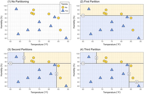
Consider the data plotted in Figure 1. The triangle in the top-left corner of all the panels depicts a case when the humidity was just over 95%, the temperature was 63 degrees Fahrenheit (^∘F), and companions did play tennis. The three circles to the right of this observation indicate three times the companions did not play tennis, when the temperature was 71–72^∘F and the humidity percentage was in the low-to-mid 90s. The model building goal underlying the CART algorithm is to recursively partition or split the two-dimensional space spanned by the temperature and humidity variables (the feature space) so that the observations are classified as either “Yes, play tennis” or “No, do not play tennis.” Successive partitions are added, one at a time, to optimize some performance metric. In our example, we will try to maximize classification accuracy (the percentage of correctly classified observations).

Fig. 1 Recursive partitioning example used to predict whether a person will play tennis or not depending on the temperature and humidity. Integers in squares indicate the order of the partitioning. Blue areas represent predictions of “Yes,” yellow areas represent predictions of “No.”

2.1 Model Building for Classification Trees

The baseline classification model with no partitioning (displayed in Figure 1; Panel 1) predicts the same classification for all the observations. The classification accuracy in this model is equivalent to the base rate of the dominant class in the observations, as this maximizes the classification accuracy. For the example data, this results in classifying all the observations as “Yes, play tennis,” which produces a classification accuracy of 57.1%. (If the algorithm had classified all observations as “No, do not play tennis,” then the classification accuracy would have only been 42.9%.)

Figure 1 (Panel 2) shows a partitioning corresponding to a single decision rule. The partition is determined after considering all possible horizontal and vertical bisections of the feature space, classifying one side of the bisected space as “Yes, play tennis” and the other side as “No, do not play tennis.” Realizing that no single horizontal or vertical bisection can perfectly classify the observations, the first partition is placed so that the model correctly classifies as many cases as possible, optimizing the classification accuracy. The optimal prediction accuracy is achieved by distinguishing between the cases that have humidity above and below 88%. The corresponding decision rule asks, “Is the humidity less than 88%?” If so, then the model predicts “Yes, play tennis.” If not, then the model predicts “No, do not play tennis.” The decision rule can be written as an IF-THEN-ELSE statement (Figure 2; Panel 1). With this rule, the model has classified 11 of the 14 cases correctly (78.6% accuracy). When compared to the classification accuracy from the baseline model (57.1% accuracy), this model has higher classification accuracy in exchange for greater complexity.

Fig. 2 Corresponding prediction rules for recursive partitioning depicted in Figure 1.

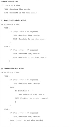
The CART algorithm is now repeated separately for each of the two partitioned sets of data with the goal of further improving the classification accuracy. For example, for the cases where humidity was less than 88%, we might ask: “Is the temperature less than 84^∘F?” If so, the model classifies cases as “Yes, play tennis;” if not, the classification is “No, do not play tennis.” For the cases where humidity was greater than (or equal to) 88%, the next decision rule is: “Is the temperature less than 67^∘F?” If so, the model classifies the cases as “Yes, play tennis;” if not, the classification is “No, do not play tennis.” This second partitioning is shown in Figure 1 (Panel 3). Again, the decision rules can be presented as a set of nested IF-THEN-ELSE statements (Figure 2; Panel 2). This results in 13 out of the 14 cases (92.9%) being correctly classified. Notice that the rules are hierarchical in the sense that the first rule precedes both of the rules in the second set. Also, by including the second set of rules, the result is a more complex model with improved classification accuracy.

Finally, we could add one more partitioning for cases where the humidity is less than 88% and the temperature is higher than 84^∘F. This rule might say, “Is the humidity less than 65%?” If so, the model classifies cases as “Yes, play tennis,” and if not, it classifies them as “No, do not play tennis.” This final partitioning is shown in Figure 1 (Panel 4), and the final set of IF-THEN-ELSE statements is shown in Figure 2 (Panel 3). At this point, the CART algorithm for model building is complete because no additional partitions can be added that will increase the classification accuracy. All 14 cases are correctly classified for 100% accuracy. Again, this is an even more complex model and an improvement in classification accuracy from the second set of rules based on the training data.

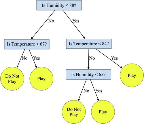
The set of decision rules is often depicted graphically as a tree diagram, which resembles an upside-down tree, hence, the origin of the terms classification tree or decision tree. Figure 3 shows the tree diagram for the hierarchical set of rules expressed by the CART algorithm to optimally classify the tennis data.

Fig. 3 The decision tree indicates a set of partitioning rules (algorithm) for predicting whether a person will play tennis or not depending on the temperature and humidity. The terminal nodes of “Play” and “Do not play” are predictions made by the model.

2.2 Model Evaluation for Classification Trees

When a single dataset is used to both build and evaluate the model, the estimated performance is often too optimistic; there is often diminished model performance when the model is evaluated on a new set of data. This phenomenon is called overfitting. For example, while the classification tree built to predict tennis outcomes resulted in a classification accuracy of 100%, it is unlikely that the accuracy would remain this high if the same set of decision rules were used to classify a new set of data. In other words, the model is likely overfitted to the data used to build the model. One method of alleviating overfit is to select a less complex model by omitting one or more rules (tree pruning; e.g., Hastie, Tibshirani, and Friedman 2009).

Typically, tree pruning is performed by cross-validation (e.g., Hastie et al. 2009), which initially (before building the model) randomly splits the entire dataset into a training set (which is used to build the model) and a validation set (which is used to perform the tree pruning). In practice, a sample may be too small to produce reasonably sized splits. In the latter case, tree pruning is performed on the entire dataset.

When pruning a classification tree, the classification accuracy of two nearly identical models are compared: one model with a particular rule excluded (pruned) versus another model with the same rule included (unpruned). If the difference between the classification accuracies of the pruned and unpruned trees is smaller than some pre-specified threshold, the decision rule is dropped, and the less complex (pruned) model is selected. Pruning can be thought of as “undoing” rules from the model building process that do not adequately improve classification accuracy, and the process is conducted starting from the “leaves” of the tree (i.e., the rules that were added the latest in the model building process).

The result of tree pruning is typically a simpler model that does not decrease prediction accuracy for out-of-sample cases. In other words, if the pruned model were to be applied to a new set of data, the classification accuracy would likely have similar performance to the data used to build the model; the classification accuracy for an unpruned model would likely be lower for the new sample than for the training data. This is similar to model evaluation with probabilistic models in which the performance of the model is weighed against its complexity, through either evaluating effects as they are added to the model or trimming the model after the fact.

In the tennis example, suppose a 10% threshold is chosen for the pruning process. Starting with the last rule that was added in the model building process (Figure 1, Panel 4), we compare classification accuracies with and without the rule (100% and 92.9%, respectively). Including this rule improves classification accuracy by 7.1%, which does not meet the 10% threshold. Therefore, the pruning process would lead us to drop this rule.

The pruning process proceeds up the hierarchy to evaluate the next set of rules (Figure 1, Panel 3). The classification accuracies of models with and without the rule distinguishing between temperatures less and greater than 84^∘F for the cases where humidity was less than 88% are 85.7% and 92.9%, respectively. Including the rule improves accuracy by less than 10%, so again the rule is not retained. When humidity was greater than 88%, distinguishing between temperatures less and greater than 67^∘F yields only one additional correctly classified case, for an improvement of 7.1%; this rule is pruned as well.

Continuing up the hierarchy, we consider the classification accuracies with and without the rule that distinguishes between humidity above and below 88% (Figure 1, Panel 2; 78.6% and 57.1% accuracy, respectively). The difference of 21.5% is greater than the 10% threshold, so this rule is retained, and the pruning process ends on this “branch” of the tree. (If there were rules higher up in the hierarchy, these would be retained as well.) The final “pruned” model is much less complex, and has fewer rules (corresponding to fewer partitions in Figure 1, Panel 2). The tree depicted in Figure 4 illustrates the final pruned model.

Fig. 4 The decision tree after pruning using a 10% inclusion threshold.

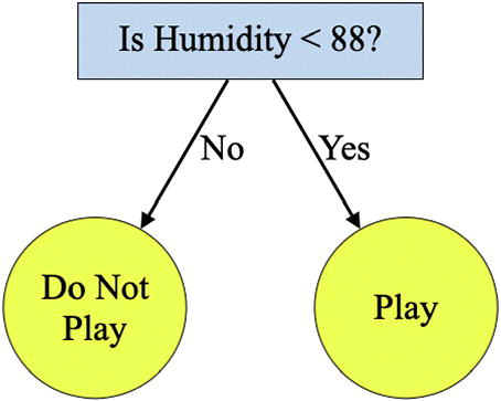
Note that a different final model might have been chosen if the pruning process had been applied to a hold-out validation set of data, or if a different threshold had been established a priori. For example, if the threshold had been 5%, all the rules would have been retained and the final model would have matched that in Figure 3.

2.3 Comparison of Algorithmic and Probabilistic Modeling Techniques

The classification trees described above are one algorithmic modeling method that can be employed when the response variable is binary. One probabilistic model that can be used with binary response variables is logistic regression. Using logistic regression with the tennis example, two predictor variables (humidity and temperature) would be used to predict the probability of playing tennis. One of the major differences between the logistic model and the classification tree is how the data generation process is defined.

Breiman (2001) described a metaphor of the data generation process as a black box (nature) operating on a set of input variables (x) to produce one or more response variables (y). Mathematically,(1) $$\mathbf{y}=f\left(\mathbf{x}\right),$$(1) where the function f represents nature’s unknown mapping of x to y. He goes on to state that in statistical modeling, be it probabilistic or algorithmic, the goal is to “extract some information about how nature is associating the response variables to the input variables” and to “predict what the responses are going to be to future input variables” (199). Probabilistic and algorithmic models take two different approaches to these tasks.

When building a probabilistic model, a stochastic component is assumed for f as a representation of the data generating process. This then serves as the basis for all further model inquiry including parameter estimation, tests, prediction, etc. As such, a primary focus in building a probabilistic model is choosing the data-generating model. For example, in the logistic model, besides having to make decisions about the model’s function form (e.g., main-effects, interaction), we also have to define the error-generating process (typically that the errors are binomially distributed).

Algorithmic models attempt to mimic nature’s mapping by using an algorithm (e.g., decision trees, neural nets) that transforms x into y. In direct contrast to building a probabilistic model, the data generating process when building an algorithmic model is not typically of interest—in many cases it is considered to be complex and unknowable (Breiman 2001). Of more interest is typically the algorithm-generated outcomes. Thus, the classification tree is concerned with only if we can correctly predict whether a person plays tennis, or not, and the model is simply the set of decisions that compose those predictions; it is a product of the data only, not the underlying data generation process.

If the goal of instruction is to teach broader principles and ideas of statistics such as statistical modeling, doing so with probabilistic models adds a lot of baggage. The process of model building and evaluation for both algorithmic and probabilistic models includes making decisions during the model building process (e.g., variables to include, the estimation procedure or algorithm used), evaluating any candidate models using a performance metric that weighs the fit of the model to the data against its complexity, and then selecting one or more models as a by-product of this evaluation. This process is described in Table 1 for both the classification tree (algorithmic) and logistic regression (probabilistic) models using the tennis example.

Table 1 Model building and evaluation process for classification tree and logistic regression using the tennis example.

Process	Classification tree	Logistic regression
Model building	Determine set of candidate predictors (Humidity, Temperature)	Determine set of candidate predictors (Humidity, Temperature)
	CART algorithm outputs set of decision rules to classify cases as “plays tennis” or “Does not play tennis”	Maximum likelihood (or other estimation method) outputs coefficient estimates and dispersion parameters based on a specified functional form and link function. The estimates can be used to determine the probability of “playing tennis”
Model evaluation	Decision rules are retained/pruned by comparing the model evaluation metric for the classification tree that includes that rule to one that does not	Predictors are retained/omitted by comparing the model evaluation metric for the logistic regression model that includes that predictor to one that does not
	Model evaluation metric is a measure of how well the cases were classified (e.g., percentage of correct classifications), often on a validation set of data	Model evaluation metric is typically a p–value. Sometimes it is some other global index of model performance (e.g., AIC, proportion of deviance explained). While cross-validation can be used, it rarely is used in traditional presentations

2.4 Summary and Study Purpose

Modern statistical science relies heavily on methods using algorithmic models, whereas teaching data analysis at the secondary level has primarily focused on probabilistic models. Research on students’ understanding of statistical modeling is dominated by probabilistic modeling approaches. While the process of statistical modeling is similar when using algorithmic or probabilistic models, algorithmic modeling does not require understanding a variety of candidate probability models in order to specify the data-generating process. However, introducing algorithmic models also means introducing methods and concepts that are likely unfamiliar to secondary teachers (e.g., classification trees, recursive partitioning, cross-validation).

Little is known about how learners come to understand algorithmic modeling, or the extent to which algorithmic modeling approaches may or may not facilitate understanding of statistical modeling, more generally. The primary goal of this study is to explore the extent to which secondary statistics teachers appear to understand ideas of model building and evaluation when introduced using classification trees.

3 Methods

Thirteen in-service secondary teachers were video-recorded as they engaged in eight group-based professional development (PD) activities. The PD, administered over five days, was designed to develop the teachers’ understanding of the process of statistical modeling (model building and evaluation) using classification trees. Nine of the 13 participants attended all of the PD sessions. The study obtained approval from the University of Minnesota’s Institutional Review Board (Proposal STUDY00003935) and Pacific Lutheran University’s Human Participants Review Board (Proposal #57).

3.1 Participants

Each of the study participants teaches statistics as part of the University of Minnesota College in the Schools (CIS) program. CIS enables secondary teachers to offer University of Minnesota courses in their secondary schools (Zieffler and Huberty 2015). The CIS Statistics course uses the CATALST curriculum (Garfield et al. 2012; Justice et al. 2020) which teaches statistical modeling through a simulation-based approach to statistical inference. The teachers—seven males and six females—had a broad range of teaching experience (6–34 years), and all but one had a Master’s degree in Curriculum or Mathematics Education. Their statistics-specific backgrounds varied with respect to number of college-level statistics courses completed (1–3 courses), years of teaching any statistics course (1–19 years), and years teaching the CIS Statistics course (1–3 years).

Through the CATALST course, the teachers experienced probabilistic modeling in many contexts related to statistical inference. The teachers built models to conduct one-proportion hypothesis tests, conducted randomization tests to assess whether there are differences between two groups (with both categorical and quantitative response variables), and used bootstrapping techniques to estimate effect sizes. The modeling was almost ubiquitously conducted using TinkerPlots^TM software to model random phenomena. It is important to note that their exposure to modeling through the course was focused on model explanation (understanding underlying random phenomena) rather than on prediction. There were no prior course activities or PD activities devoted to prediction before those described in this study, and it is likely that very few had exposure to formal training in modeling devoted to prediction.

3.2 Development and Delivery of the PD Activities

The PD activities were developed to introduce participants to some of the ideas underlying classification trees using the CART algorithm. While the prima facie statistical context of these activities involved classification trees, underlying this was exposure to more generalizable processes of modeling such as model building, model evaluation, and model selection as a by-product of model evaluation. All of the PD activities and assignments were delivered in face-to-face (not online) sessions.

The design of the PD activities was guided by constructivist frameworks of cognitive development that suggest that learning can be shaped and developed both by prior knowledge that learners hold as well as by new experiences that may be designed to foster learning. In developing the PD activities, we used principles of constructivism in education, which according to Cooper (2007) include: (i) new learning is dependent on prior knowledge; (ii) students need to be actively involved in learning; and (iii) the development of knowledge is continually changing. We also considered the Lesh and Doerr (2003; Doerr and English 2003) models and modeling perspective. Specifically, we incorporated into the PD activities the six characteristics of model eliciting activities identified by Lesh et al. (2000). To this end, we: (i) identified and used problem contexts that were expected to be of interest to the teachers; (ii) presented meaningful problems that were cognitively manageable; (iii) incorporated instructions that ensured the teachers would construct measures and models to solve problems; (iv) included prompts for the teachers to evaluate the utility of constructed measures and the performance of constructed models; (v) prompted the teachers to document the measures and models that they created in a way that could be communicated to others; and (vi) sequenced the activities so that concepts, skills, and methods developed in earlier activities were utilized and expanded upon in the new contexts of later activities.

Based on both constructivist and modeling perspectives, the teachers were expected to apply prior knowledge that they developed from their experiences with statistical modeling using probabilistic models. Teaching the CIS Statistics course gave these teachers several experiences with the statistical modeling process including building probabilistic models (Zieffler and Huberty 2015; Justice et al. 2020). They also experienced model evaluation, albeit only through the inferential decision-making lens of using a p-value to reject or not reject a model proposed in a null hypothesis. Finally, these teachers experienced statistical estimation (e.g., confidence intervals), but their experiences teaching the CIS course did not expose them to statistical ideas associated with classification. Some of these teachers, however, had additional experience with prediction (e.g., teaching Advanced Placement Statistics; see Rossman, St. Laurent, and Tabor 2015).

The PD activities provided a variety of scaffolding to support and direct the teachers’ learning, such as providing worked out examples of using a decision tree to make classifications, asking questions to elicit ideas related to classification trees and prompting connections among these ideas, and providing instructions for procedures that the teachers were not likely to develop on their own. We did not expect to identify all relevant prior knowledge that the teachers would bring to bear in learning about classification trees. Thus, we expected that the unanticipated prior knowledge would necessitate adjustments to the planned activities, as well as the development of new activities, in order to bring the set of activities within the teachers’ common zone of proximal development.

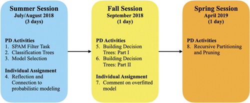
All of the PD activities were written to be completed in small groups of two to four teachers. Two assignments were also included in the materials to prompt individual reflection about some of the bigger ideas presented in the PD sessions. Each PD activity was presented to the teachers with minimal introduction (typically only to introduce the problem context). After the brief introduction, teachers were divided into small groups to work together on activities using the pedagogical approach advocated in the CATALST course (e.g., inquiry-based, activity-based, use of real data; see Garfield et al. 2012). The activities were presented in three PD sessions (see Figure 5). These activities and individual assignments are described further in the Results Section, and all of the PD materials can be found at https://github.com/zief0002/srtl-11.

Fig. 5 Timeline showing the chronology of the PD activities and individual assignments.

3.3 Data Collection and Analysis

The sequence of activities in the PD was created under the assumption that teachers, like students, are continually constructing knowledge and assimilating it with prior ideas and understandings. Subsequently, we view the teachers’ prior knowledge as a resource that can be refined and reorganized, rather than replaced, throughout the developmental process (Smith, DiSessa, and Roschelle 1993). This perspective, which underlies our analysis of the data, leads us to interpret teachers’ responses as a reflection of their developing knowledge rather than as indicators of incorrect reasoning or misconceptions.

The data collected include (i) video recordings of the teachers working in small groups on the activities, (ii) video recordings of participants presenting their results, and (iii) teachers’ work artifacts (e.g., completed activity handouts, the participants’ written reflections). The primary approach to analyzing the data was to identify themes in the participants’ reasoning, in light of the study’s purpose, by repeatedly viewing the digital recordings of the participants completing the activities and consulting accompanying artifacts. This type of methodology, related to grounded theory (e.g., Creswell 2014; Miles, Huberman, and Saldaña 2014), allows the themes, which are grounded in the data, to emerge as a product of the analysis.

As there are currently no existing frameworks for understanding the learners’ development of algorithmic thinking, a grounded theory approach was used to analyze the data. Each of the four coauthors independently viewed the video recordings and artifacts for a particular activity and group of participants, and met afterwards to discuss how the evidence might be interpreted to understand the participants’ reasoning and development. This process was repeated for each group and each activity, recording the themes about which there was consensus. Based on similarities across these records, themes emerged across groups and activities. The overall process of coming to consensus on the themes took several iterations of viewing the data and engaging in lengthy follow-up conversations to discuss what we observed. Although this analytical approach may not support strong claims about the generalizability of our findings, it allowed us freedom to investigate insights that emerged from the data (Miles et al. 2014), a tradeoff we see as valuable given the exploratory nature of the research.

4 Results

Below we lay out the educational objectives for the activities presented in each of the three PD sessions followed by our interpretation of the evidence collected from each PD session. Our interpretations of the data were framed by our experiences as statisticians, teachers of statistics, and researchers in the field of statistics education, and by the description of the model building and model evaluation processes presented earlier.

4.1 Summer PD Session

The Summer PD session—conducted over three consecutive days in summer 2018—introduced classification trees through a structured sequence of four activities intentionally designed to build the teachers’ conceptual understanding of these models and introduce ideas of the statistical modeling process. The initial activity in the PD sequence, the SPAM Filter Task, was a modification of an activity developed for the CATALST curriculum (Garfield et al. 2012). The activity introduced the teachers to global ideas of classification, in particular the use of data to inform a set of classification rules (algorithm), and the need to evaluate the algorithm’s performance. In the second activity, Classification Trees, the teachers learned to use tree diagrams based on characteristics of passengers on the Titanic to make predictions about a passenger’s fate (died or survived). In addition, the teachers learned about model evaluation by creating classification tables (i.e., confusion matrices, misclassification tables)—2 × 2 tables that summarize the number of correctly and incorrectly classified observations—and a metric of classification accuracy (e.g., percent of correctly classified observations).

Building on the ideas presented in the Classification Trees activity, the teachers next engaged in the Model Selection activity. After introducing a metric for model complexity (e.g., number of terminal nodes), teachers were asked to compare a set of models ranging in complexity and classification accuracy. By negotiating these two metrics, teachers were expected to grapple with the tradeoff between model parsimony and performance in the training data. The last assignment in the session asked teachers to reflect and comment on the perceived connections in the process of statistical modeling between the algorithmic models introduced in the PD session and the probabilistic models taught in the CIS course. Each teacher completed this reflection individually.

4.1.1 Summer PD Evidence and Findings

It did not take long for the teachers to quickly follow the logic of the classification trees. All the teachers were able to make predictions and correctly classify cases for all classification trees presented. The teachers could easily recognize which models were more complex and rank models accordingly. The teachers were also able to compute the classification accuracy for the different models. They had no trouble coming up with an accuracy measure and comparing these measures across different models.

The teachers did not, however, seem to readily understand the ideas introduced about the model evaluation process. For example, several teachers seemed inclined to evaluate the models using an absolute criterion rather than relative to the classification accuracy from the predominant class in the observed data (i.e., the classification accuracy of the no-decision baseline model). In response to whether a model with a 73% correct classification rate was a “good” model, an exemplary response would make a decision by comparing to the empirical base rate of the dominant classification (53%), which is the classification accuracy of a model that classifies all cases as one outcome. However, most groups did not consider a comparison to 53%. Some of the teachers relied on an arbitrary criterion to make this decision, typically defining “good” as approaching 100% accuracy. For example, one group of teachers decided: “It was an “ok” model. We would want something in the range of 80–90%.” Other groups justified their judgment of whether the model was “good” using knowledge from unrelated areas, such as the standard used to assign letter grades (“[70%] is a C minus”). The teachers also seemed reluctant to say the model was “good,” even after judging it better than their chosen criterion; “A model of 73% accuracy, while better than chance (50/50), doesn’t seem like the best model.”

The groups that evaluated the performance of the model by comparing it to a base rate tended to use 50% accuracy as a basis for comparison rather than the empirical base rate of the dominant classification. Perhaps these teachers were drawing from previous experiences evaluating proportions using probabilistic models in which the model underlying the null hypothesis is often assumed to have a proportion of 0.5 (e.g., fair coin models). This reasoning is not appropriate; for example, if the base rate (in the training data) and prediction accuracy of a model (on the validation data) are both 75%, the model shows no improvement over the base rate and should be pruned. However, the model could be judged as satisfactory if compared to a criterion of 50%.

We also observed the teachers drawing on their prior knowledge of statistical modeling using probabilistic models in other ways. For example, one group, in considering the level of improvement needed over the 50% criterion to say the model was better, noted, “But…what percent is acceptable? I mean, you kind of think of that p-value, that 5% is kind of that marker, acceptable, so anything less.” The teachers seem to be justifying the criterion of 0.05 pruning, by drawing from their experiences evaluating probabilistic models via statistical inference using a 0.05 level of significance. In short, some teachers may have been drawing upon their experiences in evaluating probabilistic models to evaluate what is an “acceptable” rule or a rule to prune in their algorithmic models.

The teachers also used the validation data in unconventional ways. Rather than using the validation data to evaluate the model and obtain a more accurate measure of classification accuracy, many teachers merged the training and validation data, using the larger dataset to adjust and evaluate the model. While merging the training and validation data to obtain better accuracy estimates is appropriate after the model is selected, this approach results in an overfitted model if done prior to model selection. The model was fitted to the training data, but the training data are part of the merged data, therefore the validation process was not independent of the model fitting process.

At the conclusion of the Summer PD session, we asked the teachers to reflect on connections they perceived between probabilistic and algorithmic models as a written exercise after the conclusion of the PD, which had not been previously discussed within the PD. Their written responses indicated that the teachers were mostly noting surface-level similarities. For example, one teacher responded: “…finding the percentages in the contingency tables & classification tables.” Other teachers made loose references to a course activity that uses TinkerPlots^TM software to recode outcomes using an if–then conditional procedure. Only two teachers drew connections that seemed to show a somewhat deeper understanding of the shared modeling process. One teacher, articulating the tension between model complexity and model performance, wrote:

Model performance as a concept was eye opening as we may have very high expectations. This may not be valid. I am still unsure how much complexity should be a factor. The question said if the outcomes are the same look at complexity. How close does the performance need to be?

This teacher was asking appropriate questions about the role of complexity and performance, perhaps looking for criteria that can help balance the two. Another teacher, who had a strong computer science background, also was perhaps able to touch on some of this tension:

I think the ideas of model performance & selection relate directly to the idea of building models or simulations in [the CIS course]. Students should be considering how well their models are performing based on the real-world data and understand when a more complex model is needed and when simplicity is advantageous. I think the general thinking that takes place through the work on these three models expands the conversations taking place in [the CIS course].

In the context of discussing how students should be considering model performance, this teacher pointed to when complexity may be more advantageous and when simplicity is preferred. This may suggest that the teacher recognized that model performance must be tempered by decisions about model complexity.

The Summer PD introduced teachers to several concepts and ideas underlying classification trees. Teachers seemed to grasp several of these ideas relatively quickly, including reading decision trees, using classification tree models to classify cases, recognizing differing levels of model complexity from the decision trees, and computing and comparing simple metrics of model complexity and performance. Despite their grasp of these concepts, teachers seemed to have difficulty when actually engaging in the model evaluation part of the statistical modeling process. It was not intuitive for them to evaluate a model relative to the classification accuracy from the baseline model, and many teachers instead drew on their previous knowledge from evaluating probabilistic models to compare a performance metric to an external criterion. Finally, the role of validation data in this process was also difficult for these teachers.

4.2 Fall PD Session

Ten of the teachers participated in the fall PD session. The session, conducted in one three-hour day, encompassed two activities (and a follow-up task) designed to have teachers engage in the model building and evaluation process. Unlike the activities from the Summer PD, in which teachers were presented with pre-constructed models, these two activities had the teachers build the models from data. In the Building Decision Trees activity, the teachers worked in pairs to build a model that classified whether or not a respondent supports same-sex marriage based on the respondent’s age. To keep this manageable, there were only 24 cases presented to the teachers. The second activity, Building and Evaluating an ‘Optimal’ Decision Tree, was intended to deepen the teachers’ ideas of model building by introducing a more systematic method for building classification trees: adding a single decision rule at each stage of the model building process and evaluating whether the added rule improved the model’s performance relative to some prespecified criterion. The teachers were introduced to a spreadsheet tool designed to help them make these comparisons. They were also directed to use an appropriate baseline model for evaluating their initial decision rule. This explicit instruction was included based on the observation from the Summer PD that this relative comparison did not seem intuitive to teachers.

Aside from re-emphasizing the constant negotiation between model parsimony and performance, the second activity also was designed to promote teachers’ understanding of the propensity to overfit a model to the training data. After the entire group agreed on the “best” model, they were asked to re-evaluate this model by computing its performance on 10 different validation datasets. The teachers’ understanding of this idea was probed in an assignment after the session in which they were asked to comment on the performance of a model that accurately classified a large percentage of the training cases.

4.2.1 Fall PD Evidence and Findings

Our observations of the teachers on these activities suggested they understood the link between partitioning the training set of data (presented as a dot plot) and the rules making up the decision tree. All five groups successfully created a tree from their partitioned data and also computed the misclassification rate.

Throughout the activity, there was evidence that the teachers had an awareness of overfitting. Four of the five groups built parsimonious models that incorporated between one and four rules. In their explanations for why they did not include additional rules to improve the misclassification rate, the teachers often alluded to ideas of overfit, anticipating that the misclassification rate from the validation data would be much higher. One group who initially created a model with one rule was prompted by the first author to minimize their misclassification. This group increased the complexity of their model to 10 rules (see Figure 6), which had an almost zero misclassification rate. However, when the first author commented that their model performed particularly well with the training data, the teachers replied, “Except you’re going to give us more data. And that’s going to be, we’re going to wish we didn’t do that…,” indicating some sensitivity to overfit.

Fig. 6 Partitioning of the dot plot (Panel 1) corresponding to the 10-rule overfitted model (Panel 2) created by one pair of teachers.

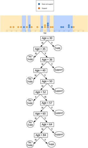
Interestingly, when the teachers went to build their trees from the rules they put in place, we observed that they did not seem to consider a hierarchy of importance within the set of rules (i.e., the first decision rule in the tree corresponds to the partition that has the lowest misclassification rate possible from all possible one-rule partitions). This approach is not conducive to pruning, a process that starts from the bottom of the tree. Even the groups that initially identified the optimal partition in the data often created a tree where this was not the first rule. In fact, the trees from all groups with multiple decision rules presented their rules in order of age (see Figure 6).

In the second activity of the PD session, we tried to build up ideas around the hierarchy of rules to support evaluation and selection of a generalizable model. The evidence here pointed to the fact that, when guided, teachers were able to produce a tree that was consistent with the idea that rules are added to the tree in descending importance based on the improvement of the misclassification rate.

During a whole group discussion, some of the teachers seemed to question the validity of the model in Figure 6 because some of the decision rules did not “match their intuitions.” During this discussion, the conversation took the following direction:

Connie: Actually, I just think we need a bigger dataset.

Mary: I agree.

Karen: I would feel better if we had more data. 24 points.

Mary: Yeah, 24 data points is not enough, not enough sample.

Connie: I don’t need my intuition, necessarily, just more data.

This may indicate that some of the teachers thought that a larger dataset would produce an initial model that would better match their intuitions, which may not necessarily be the case (e.g., the resulting model is still likely to be overfitted to the data). It also suggests that the teachers again struggled during the model evaluation stage. While they could use the validation data to correctly compute the misclassification rates for each of the trees created by removing the least important rule, they struggled with how to make use of those rates to evaluate individual rules.

Another example situation where intuitions may have been at play occurred during a discussion about whether age is a helpful predictor of whether or not a respondent supported same sex marriage. When considering a “no decision” rule where all cases are classified as “do not support” (which has only a 35% misclassification rate), one teacher said, “Nobody supports? That makes me sad!” The discussion about the best model for the data was influenced by prior beliefs about the context.

The Fall PD activities were designed to engage teachers in the model building and evaluation process, introducing ideas of building classification tree models from data and evaluating models by comparing a model’s performance with and without a rule included. These activities also introduced ideas of using cross-validation in the evaluation process. Teachers were successful in building classification trees from the raw data (presented as a dotplot) and seemed to understand how partitioning the raw data connected to the decision rules that composed the classification tree. They were also able to compute metrics of model performance.

Again, model evaluation seemed more difficult for these teachers, despite their seeming to understand broader ideas of this part of the process (e.g., they alluded to overfit). In initially building their models, they did not seem to consider a hierarchy of importance within the set of rules. However, they were successful in this endeavor once we introduced more explicit instruction asking them to attend to this hierarchy. They also struggled with the nuances of how to use performance metrics in evaluating decision rules and used their intuitions about the data’s context to override the empirical results.

4.3 Spring PD Session

The final PD session introduced the teachers to the underlying algorithm for building classification trees—recursive partitioning. Administered in one three-hour session, this activity reaccentuated many of the model building ideas introduced in the previous PD session. Because the teachers were inclined to let their intuitions override empirical results in the fall PD activities, we removed problem context to help the teachers focus on the mechanics of building the algorithm.

This activity was divided into two parts. The teachers worked in pairs in Part I. A scatterplot of training data similar to Figure 1 (Panel 1), but without context (the x-axis and y-axis were labeled X1 and X2, respectively), was used to illustrate how to create a hierarchical set of binary partitions. This process highlighted that the initial rule had the most impact on the model’s performance and that each subsequent rule, although improving the overall performance, had a diminishing effect thereon. As each partition was added, the activity illustrated how the partition was represented in a corresponding classification tree, building up the tree with each new partition. In this way, the teachers were introduced to the hierarchical nature of rules in the tree (rules at the top of the tree are “more important” or have more impact on accuracy than those at the bottom of the tree). After no further partitions could be added, Part I introduced tree pruning, demonstrating how a validation set of data would be used to trim rules starting from the bottom of the tree. This was designed to re-emphasize the idea of model parsimony and the need to evaluate a model’s performance on a validation set of data.

Part II of the activity had the teachers work in groups of three or four participants with a different training set of data and scatterplot to apply the partitioning methods demonstrated in Part I. After creating all partitions and building the corresponding decision tree, each group used a validation dataset to apply the pruning method illustrated in Part I.

4.3.1 Spring PD Evidence and Findings

The activity started out with a picture of the scatterplot that had no partitions. The teachers, working in pairs, were asked to identify a first partition that would produce the highest accuracy. All of the pairs agreed on the same optimal partition. The teachers proceeded to follow the illustrations in the handout with the result that all of the groups produced similar partitions and built similar decision trees.

When evaluating the models, different approaches to pruning emerged across the groups even though they had the same instructions. Some groups removed a rule and computed the accuracy for the reduced model, where other groups considered how removing a rule affected the accuracy in each subregion. There was also confusion over what was meant by the “least important” rule even though the instructions stated:

The first decision rule in the tree was the most important in that it provided the highest initial classification accuracy. The second set of decisions was then next most important, and so on down to the last set of decision rules. The idea of pruning is that we prune, or trim, decision rules from the tree starting with the least important rules (the last rules added).

Responding to questions from several teacher pairs on how to identify the least important rule, the first author referred everyone back to the above definition in the handout, which appeared to clear up any confusion.

As intended, the teachers focused on classification accuracy when evaluating which branches to prune. However, the teachers’ interpretations of how to prune the trees were still influenced by their prior knowledge, resulting in deviations from the pruning method illustrated in the handout. For example, Alex and Monty came up with additional criteria for what constitutes the least important rule: (i) affects the fewest number of cases and (ii) is the most inaccurate. Monty later wondered if the validation dataset could be used to not only prune, but to add new decisions to the model (i.e., to use the validation dataset as a new training dataset). Alex responded that the computer would not do this, so they could not. As another example, Connie and Mary started by using the training dataset to prune, which was pointed out to them as incorrect by the first author, and they switched to the validation dataset. However, Connie and Mary used a forward adding of rules approach (e.g., compute the accuracy for Rule 1 only, then for Rule 1 and Rule 2, etc.) instead of the demonstrated backward pruning method. In addition, some teachers were not sure how to proceed when there were two decision rules at the same level or stage of the decision tree. These points of confusion provided an opportunity for the PD leaders to facilitate discussion to help develop the teachers’ understanding of tree pruning.

For Part II, the 11 teachers were divided into three larger groups. In all three groups, the teachers worked together to identify the optimum partition at each stage or level of the model with a new training dataset. All three groups produced structurally similar decision trees that had three levels (see Figure 7), although they did not select the same cut points for each rule.

Fig. 7 Initial tree diagrams (first column) and pruned tree diagrams (second column) produced by each group or teachers during the second part of the spring professional development session.

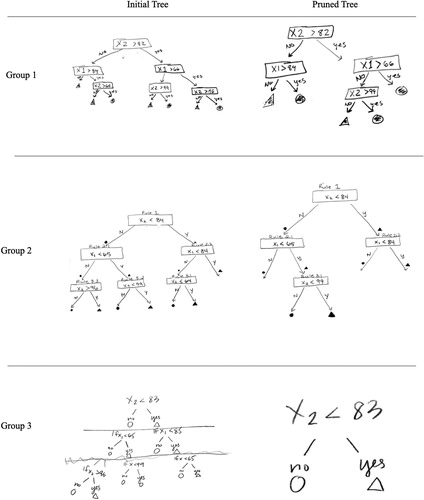
The three groups did not use the same process to trim their full decision tree model. The first group consisting of James, Tonya, and Tom conducted the pruning process according to the instructions in the Part I activity. They first calculated the accuracy rate for applying the full model to the validation dataset. They then considered how eliminating each of the level-three rules, one at a time, affected the accuracy rate. They determined that eliminating one of the level-three rules did not change the accuracy, so they eliminated that rule. They also determined that eliminating another level-three rule improved the accuracy by five percentage points. Elimination of the third level-three rule reduced accuracy by five percentage points, so that rule was kept and they recognized this necessitated keeping the level-two rule from which it branched. They found that eliminating the other level-two rule reduced accuracy, so it had to be kept. No more rules could be pruned at that point, resulting in the selected model presented in Figure 7.

The second group consisting of Beverly, Mary, Anne, and Connie did not use the backward elimination process described in Part I. Similar to Connie and Mary’s approach in Part I, they considered the accuracy of subsequently more complex models with the validation dataset, building the next model by adding the rules in the exact same sequence as they were added when building the full model with the training dataset, regardless of whether or not the next model increased accuracy. Therefore, they only considered the accuracy of six nested models and not the full set of 11 reduced models. While they selected a pruned model that was similar to that of the first group with the highest possible accuracy, their approach would not always produce this result. They also missed the opportunity to identify simpler models with the same level of accuracy as more complex models.

The third group (Josh, Alex, Monty, and Karen) used a forward model-building method somewhat similar to that of the second group, except that they started with a first model that included only their level-one rule. Then they created a second model by adding both level-two rules and a third model by adding all three of the level-three rules. They did not consider how individual rules at each level of the model affected accuracy with the validation data. They found that all three models produced the same accuracy, so they concluded that all rules after the first rule should be trimmed. If they had used the backward pruning method correctly, they would have pruned back to and selected a more accurate model that had the same structure as the first group’s (James, Tonya, and Tom) selected model.

The Spring PD activities were designed to help teachers further understand model building by introducing recursive partitioning and to improve understanding around ideas of model evaluation through continued practice with model pruning and working with validation data, two concepts from the Fall PD session that were not well understood. Teachers were successful, with some guidance, in using the ideas of recursive partitioning to build an initial model. They also were better able to evaluate individual rules using performance metrics. However, the groups took on different strategies for using the results of this evaluation for model selection. One group used the backward-elimination algorithm highlighted in the activities. Another group used a forward-selection strategy, which was not included in the activity. The third group used a forward-selection strategy, but they deviated from the algorithm by evaluating rules in totality, rather than in subsequent steps.

5 Discussion

In this study, we set out to explore the extent to which secondary statistics teachers appear to understand ideas of model building and model evaluation when introduced using classification trees. In-service, secondary mathematics teachers who had little to no previous exposure to algorithmic models were able to quickly understand and work with classification trees. They also seemed to understand more technical ideas of model building (e.g., recursive partitioning) with some scaffolding.

The ease by which the teachers were able to create, use, and interpret the trees is in contrast to the difficulties encountered in statistical modeling with probabilistic models documented in the research literature (e.g., Noll and Kirin 2016). It is possible that classification trees came easily to teachers because it did not involve some of the difficult prerequisite concepts that probabilistic modeling requires (e.g., distribution, Watson 2009; variation, Reid and Reading 2008). Moreover, our introduction to classification trees was not embedded in an introduction to statistical inference, which involves reasoning about difficult topics such as samples (Watson 2004) and sampling distributions (delMas et al. 1999). While we acknowledge that many of the difficulties with probabilistic models are likely related to the fact they are entangled with statistical inference, the positive findings in this study support that it is possible, in a short time, to build the teachers’ literacy about algorithmic models.

Ideas of model evaluation were more difficult for these teachers. While the teachers were able to easily compute measures of model performance and complexity and compare given models on these metrics, they did not initially seem to contextualize these comparisons when they were evaluating models they built. Not surprisingly, many teachers evaluated model quality by judging the model’s classification accuracy against an absolute criterion rather than comparing it to that from the baseline model. Those teachers who did make a relative comparison typically used the base rate of 50% as their basis for comparison, perhaps drawing on their previous knowledge and experiences using probabilistic models in statistical inference where the 50-50 model is often the null hypothesis used to test proportions. We also saw indication of prior knowledge playing a role when some teachers justified the quality of their model by suggesting they had a misclassification rate less than 0.05, accompanying this decision with vague references to p-values.

The introduction of cross-validation seemed to add another layer of discomfiture. Despite teachers acknowledging that models were sometimes (obviously) overfitted to training data, and perhaps recognizing the need to evaluate models using a different validation dataset, there was still confusion about how to appropriately use training and validation data. The teachers often ignored the idea that the model should be evaluated on an independent set of data, sometimes merging the two into one larger dataset or wanting to use the validation dataset to modify the model. In practice, statisticians sometimes merge the training and validation data at the end of an analysis, to obtain better estimates and then evaluate the resulting model on an independent hold-out set of data to get an idea of its predictive accuracy, but this did not seem to be the intent of the teachers, who voiced a desire for “more data” during both the model building and evaluation processes.

5.1 Implications for Teaching

The results from this study provide some preliminary evidence for using algorithmic models as a vehicle for introducing ideas of statistical modeling. First, our findings suggest that many aspects of classification trees may be quite intuitive. Over the course of just a few PD sessions, teachers who had little or no previous exposure to classification trees showed basic fluency with these models (e.g., reading and building classification trees, evaluating the complexity of the models, using the models to make classifications).

The intuitive nature of classification trees and use of simple performance measures such as classification accuracy may allow the students’ cognitive resources to be spent on understanding the process of statistical modeling. By the end of the PD sessions, we found that the teachers were describing ideas of statistical modeling that were not apparent in their work with probabilistic models (see Justice et al. 2018). We speculate that some of this is because in working with probabilistic models, ideas of statistical modeling might be obscured due to the difficulties encountered in understanding the core logic of inference (e.g., Cobb and Moore 1997; Chance, delMas, and Garfield 2004; Holcomb et al. 2010; Aquilonious and Brenner 2015; Case and Jaccobe 2018).

Finally, multivariate reasoning, a core focus of the GAISE recommendations, may be easier to achieve when using algorithmic models. We found that teachers had little to no difficulty interpreting and making classifications using models that used many variables. Even the simple tennis example, introduced earlier, includes relationships among three measures; temperature, humidity, and whether or not the person played tennis. Moreover, the conditioning that stems from including decision rules in classification (i.e., statistical interactions) seems an intuitive way to engage students in thinking about multivariate relationships.

5.2 Implications for Future Research

There are still many open questions about how introducing ideas of statistical modeling with algorithmic models impacts students’ learning and understanding. Some questions are related to how experience with probabilistic models may affect understanding of algorithmic models. For example, would teachers who had less experience with statistical modeling take the same approaches to the classification tree tasks? Would any topics in algorithmic modeling be more (or less) readily grasped by teachers who had less experience with probabilistic models?

Other questions arise from the other direction: namely, how experience with algorithmic modeling might affect understanding of probabilistic models. Could an introduction to algorithmic models illustrate principles of statistical modeling that may help pave the way for students’ understanding of probabilistic models? Or, might algorithmic modeling concepts end up conflating probabilistic modeling concepts?

Lastly, as one astute reviewer pointed out, there may be some question about whether some of the difficulties students encounter with probabilistic models may be tempered by using a regression-based approach to these models. While we see the merit in this, regression (if it is introduced at all) is generally not encountered until late in an introductory statistics course. It would be interesting to study whether introducing regression early in the course and using that as a basis for statistical inference brings the same difficulties for students, or whether the entanglement with statistical inference is indeed the issue.

With the rise of algorithmic modeling in industry, there is a case to be made that algorithmic modeling should be taught in the statistics curriculum. This raises the question: where in the curriculum could algorithmic models be sequenced? If offered early in the curriculum, how might this help or hinder the students’ understanding of probabilistic models? While our classroom and research experiences make us believe algorithmic models could precede probabilistic models (or at least statistical inference), we do not have empirical evidence that this sequence better supports students’ understanding of statistical modeling, nor whether this would improve students’ reasoning about using probabilistic models.

The scope and sequence of activities to introduce ideas related to the statistical modeling process could also be studied further. It is unclear, in reflection, if some of the struggles that teachers experienced with ideas of model evaluation were artifacts of the PD that was developed for this study. In particular, we point to more thought around how and when to introduce ideas of cross-validation. Further research could build on this work to implement and evaluate alternative learning trajectories.

As the use of algorithmic models continues to grow in statistical practice, we suggest that there is a need to study whether there may be a place for these methods to be introduced earlier in statistics curricula. While we do not believe that algorithmic models are a panacea for teaching statistical modeling, the intuitive nature of some of these models, such as classification trees, seem to make them prime candidates for inclusion in the secondary (or even primary?) grade levels. We look forward to future research that can develop an increased understanding about the role these models may play in future students’ statistical education.

Notes

1 We include only enough detail about algorithmic modeling to understand the study, and we refer the interested reader to more comprehensive descriptions in Breiman (2001) and Shmueli (2010).

References

- Aquilonious, B. C., and Brenner, M. E. (2015), “Students’ Reasoning about p-Values,” Statistics Education Research Journal, 14, 7–27. Available at https://iase-web.org/documents/SERJ/SERJ14(2)_Aquilonius.pdf.
- Bargagliotti, A., Binder, W., Blakesley, L., Eusufzai, Z., Fitzpatrick, B., Ford, M., Hutching, K., Larson, S., Miric, N., Rovetti, R., Seal, K., and Zachariah, T. (2020). Undergraduate learning outcomes for achieving data acumen. Journal of Statistics Education, 28(2), 197–211. DOI: 10.1080/10691898.2020.1776653.
- Batanero, C., Henry, M., and Parzysz, B. (2005), “The Nature of Chance and Probability,” in Exploring Probability in School: Challenges for Teaching and Learning, ed. G. Jones, New York: Springer, pp. 15–37.
- Biehler, R., Frischemeier, D., and Podworny, S. (2017), “Elementary Preservice Teachers’ Reasoning about Modeling a “Family Factory” with TinkerPlots–A Pilot Study,” Statistics Education Research Journal, 16, 244–286. Available at https://iase-web.org/documents/SERJ/SERJ16%282%29_Biehler.pdf.
- Biembengut, M. S., and Hein, N. (2010), “Mathematical Modeling: Implications for Teaching,” in Modeling Students’ Mathematical Modeling Competencies, eds. R. Lesh, P. L. Galbraith, C. R. Haines, and A. Hurford, New York: Springer, pp. 481–490.
- Breiman, L. (2001), “Statistical Modeling: The Two Cultures,” Statistical Science, 16, 199–231. DOI: 10.1214/ss/1009213726.
- Breiman, L., Friedman, J. H., Olshen, R. A., and Stone, C. I. (1984), Classification and Regression Trees, Belmont, CA: Wadsworth.
- Brown, E. N., and Kass, R. E. (2009), “What is Statistics?” The American Statistician, 63, 105–110. DOI: 10.1198/tast.2009.0019.
- Case, C., and Jaccobe, T. (2018), “A Framework to Characterize Student Difficulties in Learning Inference from a Simulation-Based Approach,” Statistics Education Research Journal, 17, 9–29, available at https://iase-web.org/documents/SERJ/SERJ17(2)_Case.pdf.
- Chance, B., delMas, R., and Garfield, J. (2004), “Reasoning about Sampling Distributions,” in The Challenge of Developing Statistical Literacy, Reasoning and Thinking, eds. D. Ben-Zvi and J. Garfield, Dordrecht, The Netherlands: Kluwer Academic Publishers, pp. 295–323.
- Cobb, G. W., and Moore, D. S. (1997), “Mathematics, Statistics, and Teaching,” The American Mathematical Monthly, 104, 801–823. DOI: 10.1080/00029890.1997.11990723.
- College Board. (2020), AP Statistics: Course and Exam Description. Available at https://apcentral.collegeboard.org/pdf/ap-statistics-course-and-exam-description.pdf?course=ap-statistics
- Consortium for Mathematics and Its Applications (COMAP) and Society of Industrial and Applied Mathematics (SIAM). (2016). Guidelines for Assessment and Instruction in Mathematical Modeling Education. Bedford, MA & Philadelphia, PA: COMAP & SIAM.
- Cooper, R. (2007), “An Investigation into Constructivism within an Outcomes Based Curriculum,” Issues in Educational Research, 17, 15–39. Available at http://www.iier.org.au/iier17/cooper.html.
- Creswell, J. W. (2014), Research Design: Qualitative, Quantitative, and Mixed Methods Approaches (5th ed.), Thousand Oaks, CA: SAGE Publications, Inc.
- delMas, R., Garfield, J., and Chance, B. (1999), “A Model of Classroom Research in Action: Developing Simulation Activities to Improve Students’ Statistical Reasoning,” Journal of Statistics Education, 7(3).
- delMas, R., Garfield, J., Ooms, A., and Chance, B. (2007), “Assessing Students’ Conceptual Understanding After a First Course in Statistics,” Statistics Education Research Journal, 6(2), 28–58. Available at http://iase-web.org/documents/SERJ/SERJ6(2)_delMas.pdf
- Doerr, H. M., and English, L. D. (2003), “A Modeling Perspective on Students’ Mathematical Reasoning about Data,” Journal for Research in Mathematics Education, 34, 110–136. DOI: 10.2307/30034902.
- Franklin, C., Bargagliotti, A., Case, C., Kader, G., Schaeffer, R., and Spangler, D. (2015), The Statistical Education of Teachers, Arlington, VA: American Statistical Association. Available at https://www.amstat.org/asa/files/pdfs/EDU-SET.pdf.
- GAISE College Report ASA Revision Committee. (2016), Guidelines for Assessment and Instruction in Statistics Education (GAISE): College Report 2016, Alexandria, VA: American Statistical Association. Available at http://www.amstat.org/education/gaise.
- Garfield, J., delMas, R., and Zieffler, A. (2012), “Developing Statistical Modelers and Thinkers in an Introductory, Tertiary-Level Statistics Course,” ZDM – The International Journal on Mathematics Education, 44, 883–898. DOI: 10.1007/s11858-012-0447-5.
- Hastie, T., Tibshirani, R., and Friedman, J. (2009), The Elements of Statistical Learning: Data Mining, Inference, and Prediction (2nd ed.), New York: Springer.
- Holcomb, J., Chance, B., Rossman, A., and Cobb, G. (2010), “Assessing Student Learning about Statistical Inference,” in Data and Context in Statistics Education: Towards an Evidence-Based Society. Proceedings of the Eighth International Conference on Teaching Statistics, ed. C. Reading., Ljubljana, Slovenia. Voorburg, The Netherlands: International Statistical Institute. Available at https://iase-web.org/documents/papers/icots8/ICOTS8_5F1_CHANCE.pdf.
- IDSSP Curriculum Team. (2019), Curriculum Frameworks for Introductory Data Science, The International Data Science in Schools Project. Available at http://idssp.org/files/IDSSP_Frameworks_1.0.pdf.
- Justice, N., Le, L., Sabbag, A., Fry, E. B., Ziegler, L., and Garfield, J. (2020), “The CATALST Curriculum: A Story of Change,” Journal of Statistics Education, 28(2), 175–186. DOI: 10.1080/10691898.2020.1787115.
- Justice, N., Zieffler, A., Huberty, M. D., and delMas, R. (2018), “Every Rose Has Its Thorn: Secondary Teachers’ Reasoning about Statistical Models,” ZDM – The International Journal on Mathematics Education, 50, 1253–1265. DOI: 10.1007/s11858-018-0953-1.
- Kaplan, J. J., Fisher, D. G., and Rogness, N. T. (2009). “Lexical Ambiguity in Statistics: What Do Students Know About the Words Association, Average, Confidence, Random and Spread?.” Journal of Statistics Education 17(3). Available at http://jse.amstat.org/v17n3/kaplan.html DOI: 10.1080/10691898.2009.11889535.
- Kula, F., and Koçer, R. G. (2020). “Why Is It Difficult to Understand Statistical Inference? Reflections on the Opposing Directions of Construction and Application of Inference Framework,” Teaching Mathematics and Its Applications: An International Journal of the IMA, 39(4), 248–265, DOI: 10.1093/teamat/hrz014.
- Lesh, R. A., and Doerr, H. M. (eds.) (2003), Beyond Constructivism: Models and Modeling Perspectives on Mathematics Problem Solving, Learning, and Teaching, Mahwah, NJ: Lawrence Erlbaum Associates.
- Lesh, R., Hoover, M., Hole, B., Kelly, A., and Post, T. (2000), “Principles for Developing Thought Revealing Activities for Students and Teachers,” in Handbook of Research Design in Mathematics and Science Education, eds. R. Lesh and A. Kelly, Mahwah, NJ: Lawrence Erlbaum Associates, pp. 591–645.
- Liu, Y., and Thompson, P. W. (2009), “Mathematics Teachers’ Understandings of Proto-Hypothesis Testing,” Pedagogies, 4, 126–138. DOI: 10.1080/15544800902741564.
- Lock, R. H., Lock, P. F., Morgan, K. L., Lock, E. F., and Lock, D. F. (2021). Statistics: Unlocking the power of data (3rd ed.). Hoboken, NJ: John Wiley & Sons.
- Manyika, J., Chui, M., Brown, B., Bughin, J., Dobbs, R., Roxburgh, C., and Byers, A. H. (2011), Big Data: The Next Frontier for Innovation, Competition, and Productivity, New York: McKinsey Global Institute.
- Miles, M. B., Huberman, A. M., and Saldaña, J. (2014), Qualitative Data Analysis: A Methods Sourcebook (3rd ed.), Thousand Oaks, CA: SAGE Publications.
- Noll, J., and Kirin, D. (2016), “Student Approaches to Constructing Statistical Models using TinkerPlotsTM,” Technology Innovations in Statistics Education, 9. Available at http://escholarship.org/uc/item/05b643r9.
- Reading, C. E., & Reid, J. (2006), “An Emerging Hierarchy of Reasoning About Distribution: From a Variation Perspective,” Statistics Education Research Journal, 5(2), 46–68. http://iase-web.org/documents/SERJ/SERJ5(2)_Reading_Reid.pdf?1402525006
- Reid, J., and Reading, C. (2008), “Measuring the Development of Students’ Consideration of Variation,” Statistics Education Research Journal, 7(1), 40–59, available at https://iase-web.org/documents/SERJ/SERJ7(1)_Reid_Reading.pdf?1402525008.
- Rossman, A. J., St. Laurent, R., and Tabor, J. (2015), “Advanced Placement Statistics: Expanding the Scope of Statistics Education,” The American Statistician, 69, 121–126. DOI: 10.1080/00031305.2015.1033985.
- Shmueli, G. (2010), “To Explain or to Predict?,” Statistical Science, 25, 289–310. DOI: 10.1214/10-STS330.
- Smith, J., DiSessa, A., and Roschelle, J. (1993), “Misconceptions Reconceived: A Constructivist Analysis of Knowledge in Transition,” The Journal of the Learning Sciences, 3, 115–163. Available at http://www.jstor.org/stable/1466679.
- Strobl, Carolin. (2013), “Data Mining,” in The Oxford Handbook of Quantitative Methods in Psychology: Vol. 2: Statistical Analysis, ed. T. A. Little, Oxford University Press, DOI: 10.1093/oxfordhb/9780199934898.013.0029.
- Tintle, N., Chance, B. L., Cobb, G. W., Rossman, A. J., Roy, S., Swanson, T., and VanderStoep, J. (2020). Introduction to Statistical Investigations. John Wiley & Sons.
- Watson, J. M. (2004), “Developing Reasoning About Samples,” In The Challenge of Developing Statistical Literacy, Reasoning and Thinking, eds. D. Ben-Zvi and J. Garfield, Dordrecht, The Netherlands: Kluwer Academic Publishers, pp. 277–294.
- Watson, J. (2009). “The Influence of Variation and Expectation on the Developing Awareness of Distribution,” Statistics Education Research Journal, 8(1), 32–61.
- Witten, I. H., Frank, E., and Hall, M. A. (2011), Data Mining: Practical Machine Learning Tools and Techniques (3rd ed.), Burlington, MA: Elsevier.
- Zapata-Cardona, L. (2015), “Exploring Teachers’ Ideas of Uncertainty,” in Reasoning about Uncertainty: Learning and Teaching Informal Inferential Reasoning, eds., A. Zieffler and E. Fry, Minneapolis, MN: Catalyst Press, pp. 95–127.
- Zieffler, A., & Huberty, M. D. (2015), “A Catalyst for Change in the High School Math Curriculum,” Chance, 28(3), 44–49.