What Quantity Appears on the Vertical Axis of a Normal Distribution? A Student Survey

Abstract

How accurately can final-year students majoring in statistics, physics, and finance label the vertical axis of a normal distribution, explain their label, identify units, and answer a question about the impact of horizontal-axis rescaling? Our survey finds that only 27 out of 148 students surveyed (i.e., 18.2%) could label the vertical axis of the normal distribution correctly, and of these, only five students (i.e., 3.4%) could explain their label. Performance on individual survey questions differed by degree program, as might be expected, but overall survey performance varied very little, ranging between only 8.8% and 12.5% of survey questions answered correctly across degree programs. Common misconceptions included labeling the vertical axis as “probability,” “count,” or “frequency.” To address these demonstrated gaps in statistics education, we give counterexamples to show why these labels cannot be correct; we explain why “probability density” is the correct label; and we give an intuitive explanation of probability density and its units. We also discuss the impact of horizontal-axis rescaling, and we indicate how the units of probability density change if the probability density function is for a bivariate or trivariate distribution instead of a univariate distribution. This article is intended for all levels of statistics education.

Keywords:

• cdf
• Linear density
• pdf
• pmf
• Probability density
• Rescaling

1 Introduction

Our primary research goal was to determine how accurately and successfully a group of final-year students majoring in statistics, physics, and finance were able to label the vertical axis of a normal distribution, explain their label, identify units of probability density, and understand the impact of a horizontal-axis rescaling. A survey instrument developed for this purpose revealed both uniformly poor student understanding and common misconceptions across degree programs. Therefore, a second (but equally important) goal emerged, namely to address the pedagogical shortfalls we identified. We do this here by providing concise explanations and examples and simple physical intuition for probability density functions (pdfs). We also give counterexamples designed to refute the most common misconceptions that were identified by our survey.

Section 2 motivates our survey and describes its construction. Section 3 summarizes the survey results. Section 4 discusses probability mass functions for discrete distributions and introduces the normal distribution. Section 5 defines probability density mathematically. Section 6 discusses units of measurement of probability density. Section 7 discusses the measurement of physical density and how to use this to build intuition for probability density. Section 8 looks at the effect of horizontal-axis rescaling. Section 9 concludes the article. The appendix contains our survey instrument, along with further discussion of implementation and outcomes.

2 Survey Motivation and Construction

Our motivation began with the casual observation that our advanced undergraduate business finance students, when given raw data and asked to present it in the form of a pdf, were unable to give a sensible answer without resorting to precanned Matlab routines that did the thinking for them. Casual follow-up discussions with our students revealed common misconceptions about the simple properties of pdfs.

Our observations are consistent with Garfield and Ahlgren (1988) who stated that “a large proportion of students, even in college, do not understand many basic statistical concepts they have studied” (p. 44). We argue, however, that a basic understanding of pdfs is part of a foundation of knowledge that is essential for success in the presentation of data, in building statistical models, and in implementing many statistical tests (e.g., for understanding p-values).

A basic understanding of pdfs is required of students and graduates in many quantitative disciplines. For example, Cohen and Chechile (1997) argued that pdfs are important beyond statistics courses or statistics text books because they are “part of the vocabulary for communicating basic ideas” (p. 2). Similarly, Falk and Konold (1999), when discussing the psychology of learning probability, argue that “probability is a way of thinking,” that “it should be learned for its own sake,” and that teaching only the minimum amount of probability required for learning statistics is a “grave mistake” (p. 151).

Although our students had many prior years of instruction, they still held onto many misconceptions about pdfs. Garfield and Ahlgren (1988) noted, however, the resilience of misconceptions in probability and statistics even after coursework designed to systematically challenge those misconceptions. They recommend techniques for overcoming difficulties in learning probability and statistics, including to recognize and confront common errors in the students’ probabilistic thinking. So, we use our survey instrument to identify common misconceptions, and then we confront those misconceptions using counterexamples and intuitive explanations. Cohen et al. (1996) took a similar approach to this. Some of their results overlap slightly with and help to explain some of our results (see our discussion in Sections 3 and 8).

At a higher level, Marshman and Singh (2017) discussed the importance of advanced undergraduate and doctoral students in physics having an understanding of and being able to manipulate probability density. Like us, they point out common misconceptions and attempt to address them. Unfortunately, their work is couched in terms of Dirac notation, and is thus too advanced for a general audience; reading our article could be assigned as a prerequisite to reading their article.

To develop a multidisciplinary survey instrument to investigate our casual observations, we chose survey questions about the distribution of human height, as approximated by a normal distribution. We chose human height because we thought it to be the simplest example that would be familiar to students across disciplines. Our survey questions could have been posed in terms of any univariate pdf, but we chose the normal distribution because of its ubiquity. For example, Batanero, Tauber, and Sánchez (2004), when discussing the students’ reasoning about the normal distribution, argue that the “normal distribution is an important model for students to learn about and use for many reasons” (p. 258). These reasons include the following: many physical, biological, and psychological phenomena can be modeled using the normal distribution; distributions such as the binomial, Student t and Poisson can be approximated by the normal distribution; Central Limit Theorem arguments mean that sample means can be assumed roughly normally distributed even when the underlying data are non-normally distributed; and, many statistical methods assume that the underlying sample is from a normal distribution.

We often have to tell our students to label the axes of any graphs they present to us. So, we reasoned that the simplest requests about a normal distribution of human height would be for the students to label the vertical axis and to explain their label. To keep the survey instrument to a single page, we chose only two other subject matter questions. The first question asks the students to identify the units of the vertical axis, and the second question asks what happens to the height of the distribution if we rescale the horizontal axis (e.g., moving from centimeters to inches).

We recognized that students in different disciplines are taught differently and with different goals, and we assumed that this would reveal itself in different responses and success rates in different questions as a function of degree program. Nevertheless (and this foreshadows the results mentioned in the next section), we discovered common misconceptions for the students from the four degree programs we targeted, and the overall proportion of incorrect answers was very similar across the students in the different degree programs surveyed. The fact that we found these common and poor results in the face of different teaching styles and goals only serves to strengthen our arguments that misconceptions about pdfs are an important multidisciplinary problem.

We asked how many probability or statistics courses the students had completed, as we expected this to differ by discipline (e.g., likely fewest in physics and likely most in statistics), and we expected success rates to be related to this count. We accepted, however, that this would likely be a messy proxy for the knowledge tested in our survey.

We gave preliminary versions of our survey instrument to a range of colleagues, and used their feedback to fine-tune both the questions and the words we would say to the students before the survey was handed out. Then we obtained ethical approval from our university to conduct our survey using hardcopy survey forms handed out by us in face-to-face classes.

The degree programs at our university have very different counts of students in their cohorts (e.g., there are six or seven times as many finance majors as there are statistics majors or physics majors). We did not take a random sample. Rather, our goal was to survey every student available to us in the degree programs we targeted; we missed only a very few who were not in class on the days we visited.

We surveyed 148 students across four degree programs. Our sample contained 130 undergraduate students in the last few weeks of the final year of their degrees (14 statistics majors, 16 physics majors, and 100 finance majors) and 18 postgraduate master of finance students in the last few weeks of their coursework.

3 Summary of Survey Results

Figure 1 summarizes the response to Question 1, where students were asked to label the vertical axis of a normal distribution (the correct answer was “probability density,” though minor variations were accepted). Only 27/148 (18.2% of students) gave the correct answer. The most common incorrect answers were “probability,” “count,” and “frequency.” We provide several counterexamples later to show why these labels cannot be correct.

Fig. 1 Answers to survey Question 1: label vertical axis.

NOTE: This bar chart shows counts (and proportions) of students giving vertical axis labels in response to survey Question 1. Of the 148 students surveyed, “Frequency” and “Count,” if combined, were the most popular incorrect responses. The single most popular incorrect answer was, however, “Probability.” The “Other” category include nonsensical answers like “Ethnicity” or “Weight” or “Kurtosis,” and also two students who left the answer blank. See also Table 2 for a breakdown of answers to Question 1 by degree program.

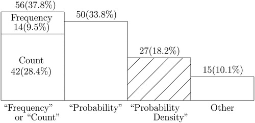
Batanero, Tauber, and Sánchez (2004) argued that students often confuse empirical distributions with fitted theoretical distributions. This may explain the popular wrong answers of frequency and count appearing in Figure 1. Similarly, Cohen et al. (1996) said that some students mistake the vertical axis of a histogram for the vertical axis of a scatterplot. We did not include any histograms, but we suspect that some of the nonsensical answers we received to our survey (see the caption to Figure 1) may be because students mistook the vertical axis of a pdf for the vertical axis of a scatterplot.

Figure 2 shows the count and proportion of students who got exactly 0, 1, 2, 3, or 4 answers correct, respectively, on the survey. As an aside, a group of eager postgraduate students came to see the second author in his office after the survey to ask what the correct answers were and why. One of the students declared that although she had seen normal distributions in the classroom for many years, she was unable to answer any of our survey questions. She is in good company, because Figure 2 shows that by far the most common result was no correct answers (105/148 students; 70.9%). Table 3 in Appendix A.1 gives some conditional details. For example, it shows that of the 27 students who could label the vertical axis of the normal distribution correctly, 15 could correctly answer no other question, 11 could correctly answer only one other question, one could correctly answer two other questions, and none could correctly answer all four questions.

Fig. 2 Number of correct survey answers per student.

NOTE: This probability mass function shows the proportion of our sample of 148 students getting 0, 1, 2, 3, or 4 correct answers, respectively, to the four questions posed in our probability density survey. Counts are shown in parentheses. The mean of 0.38 correct answers per student is indicated with a small triangle. The median number of correct answers per student was 0.

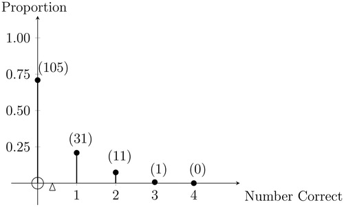
Table 3 Which survey answers students got correct.

No. Correct	Q1	Q2	Q3	Q4	Count
0	N	N	N	N	105
1	Y	N	N	N	15
1	N	Y	N	N	2
1	N	N	N	Y	14
2	Y	Y	N	N	4
2	Y	N	Y	N	1
2	Y	N	N	Y	6
3	Y	Y	Y	N	1
4	Y	Y	Y	Y	0

NOTE: This table summarizes actual outcomes to the four survey questions. “Y” means yes, the answer was correct; “N” means no, the answer was incorrect. As summarized in Figure 2, 105 students got no correct answers, $15+2+14=31$ students got one correct answer, $4+1+6=11$ students got two correct answers, 1 student got three answers correct, and no students got four correct answers. Although there are 16 possible permutations of Y and N over the four questions, we saw only the eight outcomes shown here. As mentioned earlier, only $4+1=5$ students could both label the vertical axis (Q1) and explain their answer (Q2), and only $15+4+1+6+1=27$ students could answer Q1 correctly.

Table 1 shows the proportion of correct answers by discipline and the proportion of correct answers overall. For Question 1 (label the vertical axis of a normal distribution), only 18.2% of students could answer correctly, as reported in Figure 1. The statistics majors were the best at doing so, with 42.9% answering correctly; the undergraduate finance majors were the worst at doing so, with only 12% answering correctly. This difference in proportions is statistically discernible (significant) with a p-value less than 5%.¹ Given the small subsample sizes in different majors, we cannot point to other statistically discernible differences in performance by degree program. We will say, however, that although the statistics majors were the best in our sample at labeling the vertical axis, we were disappointed that no statistics student was able to explain their label (Question 2) or answer any other question correctly.

Table 1 Proportion of students answering correctly.

Question	Statistics	Physics	Finance	MF	Overall
Q1	6 (42.9%)	4 (25.0%)	12 (12.0%)	5 (27.8%)	27 (18.2%)
Q2	0 (0.0%)	1 (6.3%)	5 (5.0%)	1 (5.6%)	7 (4.7%)
Q3	0 (0.0%)	2 (12.5%)	0 (0.0%)	0 (0.0%)	2 (1.4%)
Q4	0 (0.0%)	1 (6.3%)	18 (18.0%)	1 (5.6%)	20 (13.5%)
Overall	10.7%	12.5%	8.8%	9.7%	9.5%
N	14 (9.5%)	16 (10.8%)	100 (67.6%)	18 (12.2%)	148 (100.0%)

NOTES: This table shows the count and proportion of students giving the correct answers to the four survey questions, by degree program: statistics, physics, and finance undergraduates, and master of finance (MF). For example, with four questions asked of each student, it follows that $(4+1+2+1)/(16\times 4)=12.5\%$ of all questions asked of physics majors were answered correctly, as reported overall. N is the count of students in each program, with proportions in parentheses. See Appendix A.2 to link question numbers to question content. See also Table 2 for a further breakdown of answers to Question 1.

The incorrect answers to our survey questions outnumber the correct answers by a factor of almost 10 to 1. What the students do not know is valuable information because it can inform pedagogy and the allocation of classroom time and resources. So, we looked more closely at the incorrect answers to identify common misconceptions and to motivate our choice of counterexamples. When labeling the vertical axis, the most popular wrong answers were common to all degree programs, but with varying proportions (see Table 2).

Table 2 Breakdown of answers to Question 1 by degree program.

Answer	Statistics	Physics	Finance	MF	Overall
“Probability density”	6 (42.9%)	4 (25.0%)	12 (12.0%)	5 (27.8%)	27 (18.2%)
“Probability”	1 (7.1%)	8 (50.0%)	34 (34.0%)	7 (38.9%)	50 (33.8%)
“Count”	4 (28.6%)	2 (12.5%)	34 (34.0%)	2 (11.1%)	42 (28.4%)
“Frequency”	3 (21.4%)	1 (6.3%)	6 (6.0%)	4 (22.2%)	14 (9.5%)
Other	0 (0.0%)	1 (6.3%)	14 (14.0%)	0 (0.0%)	15 (10.1%)
N	14 (9.5%)	16 (10.8%)	100 (67.6%)	18 (12.2%)	148 (100.0%)

NOTES: This table shows the count and proportion of student responses to Question 1 of our survey (i.e., label the vertical axis of a normal distribution). The correct answer is “probability density,” and the most common incorrect answers were “probability,” “count,” and “frequency.” Some of the other nonsense answers were mentioned already in the caption to Figure 1. The data are broken down by degree program: statistics, physics, and finance undergraduates, and master of finance (MF). N is the count of students in each program, with proportions in parentheses.

Table 1 reports that two physics students were the only students in our sample who were able to correctly answer Question 3, which asked for the units of probability density in our example. Although the sample size is small, we did wonder whether this small success was because of the frequent use of dimensional analysis by physicists.

Question 4 asked whether the height of the density function changed with a change in horizontal-axis units (in our case, changing the horizontal axis from centimeters to inches). Table 1 reports some odd results. Eighteen out of 100 finance undergraduate students correctly answered the question about rescaling (Question 4). This was our only multiple-choice question, and we suspect some guessing was involved because these students were much less successful on the preceding questions (see Table 1). Nevertheless, with only four multiple-choice answers to choose from, the 13.5% of correct answers here overall (see the last column in Table 1) was still worse than would be expected by random chance alone. Question 4 is discussed further in Section 8.

Two preliminary questions on our survey asked for a count of probability or statistics courses enrolled in or previously completed. We ended up combining these counts because the survey was conducted in the final few weeks of the final semester of the final year for each student; so, we figured that the courses currently enrolled in were essentially complete. This count of courses ranged from 0 (10 students, all physics majors) to 11 (a statistics major). The mean (and median) count of probability or statistics courses taken was 6.3 (6) for statistics undergraduates, 0.5 (0) for physics undergraduates, 2.6 (2) for finance undergraduates, 4.0 (4) for master of finance postgraduates, and 2.9 (2) overall.

One would hope that performance on Question 1 (i.e., label the vertical axis) is related to the number of probability or statistics courses taken. Let C be the number of classes taken and L be the indicator variable 1 or 0 for whether the correct label was given in Question 1 or not, respectively. We found $\mathit{corr}(C,L)=24.2\%$ (t-statistic 3.01). We split the students into three groups: C < 3 (83 students), C = 3 (30 students), and C > 3 (35 students). We ran a Pearson chi-squared 3 × 2 contingency table with these splits against whether L = 1 or L = 0 (correct label or not, respectively). (This was the only sensible split on C we could make that had an expected count in every cell larger than 5.) The chi-squared test statistic was ${\chi }^2=11.1$ with 2 degrees of freedom and a p-value of 0.4%. Both the correlation and contingency results support the conclusion that more statistics classes are associated with better answers to Question 1. This result may, however, be driven by the performance of the statistics majors on Question 1 (see Table 1) and the higher number of classes taken by statistics majors (average 6.3 classes) compared with the non-statistics majors (average 2.5 classes).²

Finally, Table 1 shows that the success rate of the students from each degree program was relatively consistent, varying tightly between 8.8% and 12.5% of answers correct.

We now address the pedagogical gaps revealed by our survey. The best place to start is with probability mass functions.

4 The pmf, cdf, and pdf

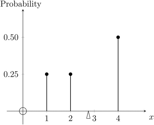
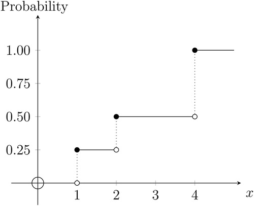
Suppose that a discrete random variable X_d has lumps of probability mass at discrete points, as shown in Figure 3. In this case, when we plot the distribution, we are plotting a probability mass function (pmf) describing where the lumps of probability mass are.³ The quantity on the vertical axis of the pmf is probability, as labeled in Figure 3.

Fig. 3 Probability mass function $P(X_d=x).$

NOTE: The discrete random variable X_d takes values $x=1,2,$ and 4, with probabilities $\frac{1}{4},\frac{1}{4}$, and $\frac{1}{2}$, respectively. The triangle marks the probability-weighted average of the distribution (i.e., the mean of 2.75); this is the location of the perpendicular axis through the center of gravity of the probability mass distribution. The corresponding cumulative distribution function appears in Figure 4.

In the univariate discrete case in Figure 3, the cumulative distribution function (cdf) given by $F_{X_d}(x)=P(X_d\le x)$ is a step function, as shown in Figure 4.⁴ So, $F_{X_d}(x)$ is not continuous, let alone differentiable, and we cannot differentiate $F_{X_d}(x)$ to get a pdf.⁵

Fig. 4 Cumulative distribution function $P(X_d\le x).$

NOTE: The discrete random variable X_d takes values $x=1,2,$ and 4, with probabilities $\frac{1}{4},\frac{1}{4}$, and $\frac{1}{2}$, respectively. The plot shows the cumulative distribution function $P(X_d\le x)$. The corresponding pmf appears in Figure 3.

If, however, X is a continuous random variable (e.g., X follows a normal distribution), then X has a differentiable cdf $F_X(x)$, and $f_X(x)=\frac{\mathrm{d}{F}_X(x)}{\mathrm{d}x}$ is the pdf. In this case, the quantity on the vertical axis of a plot of $f_X(x)$ is not probability, but probability density. The remainder of this article uses explanations and examples to provide deep intuition for what is meant by “probability density.”

The best-known continuous random variable is one that follows a normal distribution. Equation (1)(1) $$\begin{array}{c}{F}_X(x)=P(X\le x)={\int }_{t=-\infty }^x\frac{1}{\sqrt{2\pi }\sigma }{e}^{-\frac{1}{2}{\left(\frac{t-\mu }{\sigma }\right)}^2}dt,\\ -\infty <x<\infty \end{array}$$(1) gives the cdf for a normal distribution with mean μ and standard deviation σ.(1) $$\begin{array}{c}{F}_X(x)=P(X\le x)={\int }_{t=-\infty }^x\frac{1}{\sqrt{2\pi }\sigma }{e}^{-\frac{1}{2}{\left(\frac{t-\mu }{\sigma }\right)}^2}dt,\\ -\infty <x<\infty \end{array}$$(1)

This normal cdf is illustrated in Figure 5. Three points are labeled a, b, and c, respectively, for future reference.

Fig. 5 Normal cumulative distribution function $F_X(x).$

NOTE: The cdf $F_X(x)$ is illustrated for a normal distribution with mean μ and standard deviation σ (see Equation (1)(1) $$\begin{array}{c}{F}_X(x)=P(X\le x)={\int }_{t=-\infty }^x\frac{1}{\sqrt{2\pi }\sigma }{e}^{-\frac{1}{2}{\left(\frac{t-\mu }{\sigma }\right)}^2}dt,\\ -\infty <x<\infty \end{array}$$(1) ). The slope of the cdf is close to zero at points a and c and reaches a maximum of $1/\left(\sqrt{2\pi }\sigma \right)$ at point b.

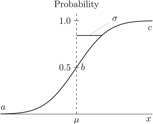
As mentioned already, from a purely mathematical standpoint, the height of a continuous pdf is the slope of (i.e., the derivative of) the corresponding cdf: $f_X(x)=\frac{\mathrm{d}{F}_X(x)}{\mathrm{d}x}$. The slope of the normal cdf is close to zero at points a and c in Figure 5, and the maximum slope occurs at point b; this maximum slope takes the value $1/\left(\sqrt{2\pi }\sigma \right)$. You can deduce the maximum slope of $F_X(x)$ by differentiating Equation (1)(1) $$\begin{array}{c}{F}_X(x)=P(X\le x)={\int }_{t=-\infty }^x\frac{1}{\sqrt{2\pi }\sigma }{e}^{-\frac{1}{2}{\left(\frac{t-\mu }{\sigma }\right)}^2}dt,\\ -\infty <x<\infty \end{array}$$(1) with respect to x, via the fundamental theorem of calculus, to obtain the slope (which is just the pdf). Then you can differentiate this slope using the composite function theorem and solve the first-order condition to deduce that an extremum slope, with value $1/\left(\sqrt{2\pi }\sigma \right)$, occurs at $x=\mu$ (i.e., point b in Figure 5). (You should calculate the second-order condition to confirm that this extremum is a maximum.)

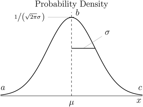
Figure 6 shows the normal pdf $f_X(x)$ corresponding to the normal cdf $F_X(x)$ in Figure 5. The functional form of the pdf plotted in Figure 6 is given by Equation (2)(2) $$f_X(x)=\frac{1}{\sqrt{2\pi }\sigma }{e}^{-\frac{1}{2}{\left(\frac{x-\mu }{\sigma }\right)}^2},-\infty <x<\infty$$(2) .(2) $$f_X(x)=\frac{1}{\sqrt{2\pi }\sigma }{e}^{-\frac{1}{2}{\left(\frac{x-\mu }{\sigma }\right)}^2},-\infty <x<\infty$$(2)

Fig. 6 Normal pdf $f_X(x).$

NOTE: A pdf $f_X(x)$ is illustrated for normally distributed X with mean μ and standard deviation σ (see Equation (2)(2) $$f_X(x)=\frac{1}{\sqrt{2\pi }\sigma }{e}^{-\frac{1}{2}{\left(\frac{x-\mu }{\sigma }\right)}^2},-\infty <x<\infty$$(2) ). The height of the pdf is close to zero at points a and c, and reaches a maximum of $1/\left(\sqrt{2\pi }\sigma \right)$ at point b.

Note that, as mentioned already, the pdf in Equation (2)(2) $$f_X(x)=\frac{1}{\sqrt{2\pi }\sigma }{e}^{-\frac{1}{2}{\left(\frac{x-\mu }{\sigma }\right)}^2},-\infty <x<\infty$$(2) is visible as the integrand in Equation (1)(1) $$\begin{array}{c}{F}_X(x)=P(X\le x)={\int }_{t=-\infty }^x\frac{1}{\sqrt{2\pi }\sigma }{e}^{-\frac{1}{2}{\left(\frac{t-\mu }{\sigma }\right)}^2}dt,\\ -\infty <x<\infty \end{array}$$(1) , but with the dummy variable t in place of x.

The exponential term $e^{-\frac{1}{2}{[(x-\mu )/\sigma ]}^2}$ appearing in Equation (2)(2) $$f_X(x)=\frac{1}{\sqrt{2\pi }\sigma }{e}^{-\frac{1}{2}{\left(\frac{x-\mu }{\sigma }\right)}^2},-\infty <x<\infty$$(2) determines the shape of the normal distribution’s pdf. Recall that as v gets larger, e ${}^v$ gets very large, and $e^{-v}=1/e^v$ gets very small, very quickly. For example, $e^{-1}=1/e^1\approx 0.368,e^{-10}=1/e^{10}\approx 0.0000454$, and$$\begin{array}{c}{e}^{-100}=1/e^{100}\\ \approx 0.0000000000000000000000000000000000000000000372\\ =3.72\times {10}^{-44}\end{array}$$

(i.e., there are 43 zeroes after the decimal point!). Thus, as x moves away from μ in either direction, the negative exponential term in Equation (2)(2) $$f_X(x)=\frac{1}{\sqrt{2\pi }\sigma }{e}^{-\frac{1}{2}{\left(\frac{x-\mu }{\sigma }\right)}^2},-\infty <x<\infty$$(2) drives the value of $f_X(x)$ down to zero very quickly and smoothly; when $x=\mu$, however, this exponential term has the least effect, and $f_X(x)$ reaches its peak. Thus, the height of the pdf $f_X(x)$ in Figure 6 is close to zero at points a and c, and reaches its peak, at a value of $1/\left(\sqrt{2\pi }\sigma \right)$, at point b, corresponding to the slopes of the cdf at the points with the same respective labels in Figure 5.

In the case where X is standard normal (i.e., μ = 0 and σ = 1), the peak height of the normal pdf is $1/\sqrt{2\pi }$, which is 0.3989 to four decimal places, or 0.40 to two decimal places. What if we consider a normal distribution with a much smaller standard deviation, say, $\sigma =0.10$? In this case, the peak height is $1/(\sqrt{2\pi }·0.10)\approx 4.0$. That is, the height of the pdf at its peak is about 4. Similarly, a standard deviation of $\sigma =0.01$ yields a height at the peak of the normal pdf of about 40. Indeed, $\sigma =1/\left(\sqrt{2\pi }H\right)$ yields a peak value of H for any arbitrarily large, finite, positive H we care to choose. We know, however, that probability can be no more than 1. So, given the existence of peak heights of the normal distribution’s pdf well beyond 1.0, this counterexample shows that the quantity on the vertical axis of a univariate normal pdf plot cannot possibly be probability.

For a second counterexample, note that there are uncountably infinitely many points on the horizontal axis in Figure 6 (Judge et al. 1988, p. 22). So, the probability that a continuous random variable assumes any particular x value must be zero. It follows that if the continuous pdf were a plot of $P(X=x)$, it would be level at zero for all x, contradicting its presentation as a bell-shaped curve in Figure 6. Hence, the variable on the vertical axis of the univariate normal distribution cannot be probability.

Our arguments above are only a starting point for understanding the vertical axis of a pdf; we provide more intuition in the following sections.

5 Probability Density

Only 7/148 (4.7%) of our survey respondents could give an intuitive explanation of what probability density is (see the last column in Table 1). The other 141/148 (95.3%) of students seemingly work with the concept frequently, but with little or no real understanding of what they are manipulating.

Suppose that we cut the probability mass under the pdf in Figure 6 into narrow vertical slices based on a discretization of the horizontal axis into small steps numbered using i. In Figure 7 we zoom in on one such slice, centered on x_i. We see that probability mass is area, not height, under the density function.

Fig. 7 Zoomed View of the ith narrow slice under $f_X(x).$

NOTE: We assume a discretization of the x-axis under $f_X(x)$ into small steps numbered using i, where x_i sits at the center of the ith small step. $f_X(x_i)$ is the height of the function f_X at x_i, $\Delta x_i$ is the width of the ith small step centered on x_i, and ${\text{area}}_i$ is the area of the ith narrow slice centered on x_i. We assume $P(x_i;\Delta x)\equiv P\left(x_i-\frac{\Delta x}{2}\le X\le x_i+\frac{\Delta x}{2}\right)$, as in Equation (3)(3) $$P(x_i;\Delta x)\equiv P\left(x_i-\frac{\Delta x}{2}\le X\le x_i+\frac{\Delta x}{2}\right),$$(3) .

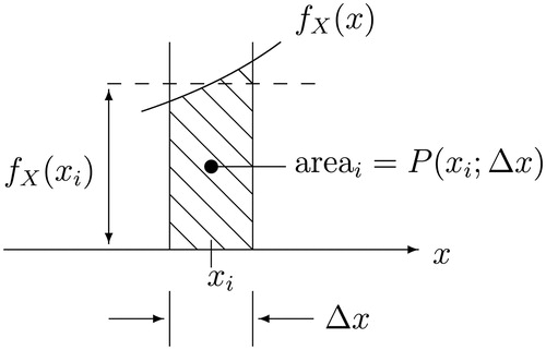
The total area under any pdf is equal to 1. So, if we define(3) $$P(x_i;\Delta x)\equiv P\left(x_i-\frac{\Delta x}{2}\le X\le x_i+\frac{\Delta x}{2}\right),$$(3) we get that(4) $$\sum _{i}P(x_i;\Delta x)=1.$$(4)

It should be clear from Figure 7 that Equation (5)(5) $$P(x_i;\Delta x)\approx f_X(x_i)·\Delta x,$$(5) must hold,(5) $$P(x_i;\Delta x)\approx f_X(x_i)·\Delta x,$$(5) with accuracy improving (in absolute terms) as $\Delta x\to 0$. That is, the shaded region in Figure 7 has an area approximately equal to the area of a rectangle of height $f_X(x_i)$ and width $\Delta x$, and the approximation gets better as $\Delta x\to 0$. Spiegel (1975, p. 42) and Ross (1987, p. 34) presented similar arguments. It follows from Equation (5)(5) $$P(x_i;\Delta x)\approx f_X(x_i)·\Delta x,$$(5) that(6) $$f_X(x_i)\approx \frac{P(x_i;\Delta x)}{\Delta x},$$(6) with accuracy improving as $\Delta x\to 0$. In words, Equation (6)(6) $$f_X(x_i)\approx \frac{P(x_i;\Delta x)}{\Delta x},$$(6) implies that univariate probability density $f_X(x)$ is the limiting value of a ratio of the size of a lump of probability mass under the density function to a length measured in units of the x-axis as that length tends to 0. We build upon this intuition in the following three sections.

Regarding this intuition, Question 2 of our survey asked the students to explain their axis label. We accepted any answer that displayed correct intuition, even if the axis label itself was incorrect. For example, if a student said that the area of a slice taken under the pdf displays the probability associated with that range of values along the horizontal axis, we accepted that as a correct definition of the vertical axis label.

Note that we have sometimes seen “cdf” used as an acronym for cumulative density function, rather than for cumulative distribution function. Comparing Equations (1)(1) $$\begin{array}{c}{F}_X(x)=P(X\le x)={\int }_{t=-\infty }^x\frac{1}{\sqrt{2\pi }\sigma }{e}^{-\frac{1}{2}{\left(\frac{t-\mu }{\sigma }\right)}^2}dt,\\ -\infty <x<\infty \end{array}$$(1) , (2)(2) $$f_X(x)=\frac{1}{\sqrt{2\pi }\sigma }{e}^{-\frac{1}{2}{\left(\frac{x-\mu }{\sigma }\right)}^2},-\infty <x<\infty$$(2) , and (5)(5) $$P(x_i;\Delta x)\approx f_X(x_i)·\Delta x,$$(5) (as $\Delta x\to 0$), however, we can see that the cdf cumulates probability, not probability density. So, “cumulative density function” could be argued to be a misnomer.

Note also that the logical arguments in this section collapse completely if the vertical axis label on the normal distribution is “probability,” “count,” or “frequency” (as given by students in Figure 1 and Table 2), because in that case there is no reason why such a function should integrate to one.

6 Units

Only 2/148 (1.4%) of our survey respondents could identify the units of measurement for the vertical axis of the normal distribution in the simple example in our survey (see the last column in Table 1). The most common answers were that the vertical axis of the normal distribution is dimensionless (42/148, 28.4%), that it is a percentage or a decimal or a fraction taking values between 0 and 1 (38/148, 25.7%), or that it is a number or a count or is in thousands or is “N” (31/148, 20.9%). These common incorrect answers accounted for 111/148 students (75%), most of whom failed to put the correct label on the vertical axis.

In fact, it is probability mass, not probability density, that is dimensionless. It follows from Equation (6)(6) $$f_X(x_i)\approx \frac{P(x_i;\Delta x)}{\Delta x},$$(6) that univariate probability density must be measured in units of the inverse of the dimension of the horizontal-axis variable. Alternatively, for probability to be dimensionless in Equation (5)(5) $$P(x_i;\Delta x)\approx f_X(x_i)·\Delta x,$$(5) , the units of the height of the rectangle (i.e., of $f_X(x_i)$) must be the reciprocal of the units of the width of the rectangle (i.e., of $\Delta x$). For example, if the pdf is of human height measured in centimeters, then probability density, on the vertical axis, is in units of 1/centimeter, or ${\text{centimeters}}^{-1}$—though we do not usually give the units on the vertical axis in a pdf plot.

There is also a direct method for deducing the units of measurement of probability density. For example, in the case of the normal density in Equation (2)(2) $$f_X(x)=\frac{1}{\sqrt{2\pi }\sigma }{e}^{-\frac{1}{2}{\left(\frac{x-\mu }{\sigma }\right)}^2},-\infty <x<\infty$$(2) , a term-by-term examination reveals that the scaling parameter σ in the denominator of $1/\left(\sqrt{2\pi }\sigma \right)$ determines the units of probability density as the inverse of the dimension of the horizontal-axis variable (note that the units all cancel out in the exponential term). This approach does not, however, work immediately for pdfs with latent scaling parameters. For example, in the case of the standard normal and Student-t, you must first consult the non-standardized normal (i.e., Equation (2)(2) $$f_X(x)=\frac{1}{\sqrt{2\pi }\sigma }{e}^{-\frac{1}{2}{\left(\frac{x-\mu }{\sigma }\right)}^2},-\infty <x<\infty$$(2) ) and the non-standardized Student-t (e.g., Wheat, Stead, and Greene 2019, eq. (4)(4) $$\sum _{i}P(x_i;\Delta x)=1.$$(4) ), respectively, to see the units directly, before imposing a standardizing transformation.

The units for bivariate or trivariate probability density are discussed in Section 7.

7 Density: Volume, Areal, and Linear

In physics, the density of a material is expressed in units of mass per unit of three-dimensional volume. For example, water (H₂O) has a density of roughly 1.00 grams per cubic centimeter, lead (Pb) has a density of roughly 11.35 grams per cubic centimeter, and wolfram (W) has a density of roughly 19.30 grams per cubic centimeter (all at ${20}^{°}$ C) (Weast 1966, pp. F-1, B-118, and B-143, respectively). For density of the population of fish in the ocean, one possible measure is the count of fish per cubic kilometer. These are all volume density figures (i.e., where we divide a count by a three-dimensional quantity).

If we measure the density of the population of persons in some city, then we are likely to use a count of persons per square mile. This is an areal density figure (i.e., where we divide a count by a two-dimensional quantity). A corn farmer’s productivity measured in bushels of corn per acre is similarly an areal density measure.

If we measure the density of a rope or a thread, then we are likely to use a measure that has grams in the numerator and meters in the denominator. For example, fiber density can be measured and quoted in denier units (i.e., the mass of the fiber, in grams, per 9000 meters) or decitex units (i.e., the mass of the fiber, in grams, per 10,000 meters). A single strand of silkworm silk has a density of roughly 1–3 denier (Kumar and Umakanth 2017) and a human hair might have a density of 75 denier (Shukla 2017, p. 31), though there is much variation. These are all measures of linear density (i.e., where we divide a count by a one-dimensional quantity).

As argued in Section 6, univariate probability density is the ratio of the size of a lump of probability mass under the density function to a length measured in units of the horizontal axis (in the limit as the length measure goes to zero). So, univariate probability density is a linear density measure, like fiber density measured in denier.

Indeed, if we go back to the normal distribution in Figure 6, we can see that as we look along the horizontal axis, the probability density near the mean (now thought of as a measure of linear density) is higher than the probability density in the tails. This is because near the mean the plot is “thicker” per unit length of the horizontal axis, the same way that a poorly made rope might be thicker per unit length in some places.

The units change for higher order density functions. For a bivariate pdf, probability density is an areal density, say, $f_{X,Y}(x_i,y_i)\approx P(x_i,y_i;\Delta x,\Delta y)/(\Delta x\Delta y)$, analogous to Equation (6)(6) $$f_X(x_i)\approx \frac{P(x_i;\Delta x)}{\Delta x},$$(6) , with units adjusted accordingly. For a trivariate pdf, probability density is a volume density measure, with units adjusted accordingly.

8 Rescaling

As mentioned already, we found that 112/148 (75.7%) of survey respondents answered our Question 4 incorrectly by saying that a change in horizontal axis units has no impact on the vertical scale of a univariate pdf. This error is consistent with the answers reported in Figure 1 and Table 2, where almost three-quarters of the respondents have mistaken probability density for probability mass, count, or frequency.

Cohen et al. (1996) also found that students had difficulty understanding the effect on the vertical height of the peak of a normal distribution if the mean and standard deviation were changed (p. 49). They suggest that the task of meeting three simultaneous constraints may have been too difficult for students (i.e., moving the mean, altering the spread, and adjusting the height of the peak so that the total area under the pdf is conserved).

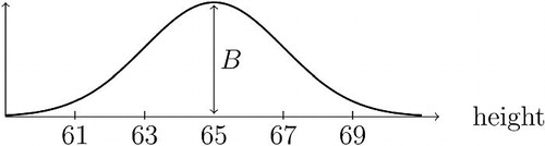
Suppose that $f_X(x)$ is the pdf of the distribution of height of female undergraduate students where X is measured in inches. Let us assume that X is normally distributed (this is likely not far from the truth). The mean is likely close to 64 inches (5 feet 4 inches). The standard deviation is likely close to two inches. The left-hand-side plot in Figure 8 shows $f_X(x)$. The height of $f_X(x)$ at its peak is likely about $\frac{1}{\sqrt{2\pi }\sigma }=\frac{1}{\sqrt{2\pi }2}\approx 0.20$ (and this is actually 0.20 ${\text{inches}}^{-1}$, though, as mentioned already, we do not typically quote the units on the vertical axis).

Fig. 8 Rescaling preserves Shape I.

NOTE: The left-hand-side density plot shows height of female undergraduates measured in inches; the right-hand-side density plot shows their height measured in centimeters (see the text). The two figures have an identical shape; all that changes are the scales on the axes. Challenge: Can you confirm that if height is instead measured in meters, we expect the peak height of the second pdf to be roughly $8{\text{meters}}^{-1}$?

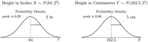
Now, suppose we let Y be the height of the very same population, but let Y be measured in centimeters instead of inches. How do the horizontal and vertical scales for $f_Y(y)$ differ from the horizontal and vertical scales for $f_X(x)$? Well, with 2.54 centimeters per inch, the mean of Y will be roughly 162.5 centimeters, and the standard deviation of Y will be roughly 5 centimeters. The right-hand-side plot in Figure 8 shows $f_Y(y)$. The height of $f_Y(y)$ at its peak is likely about $\frac{1}{\sqrt{2\pi }\sigma }=\frac{1}{\sqrt{2\pi }5}\approx 0.08$ (and this is actually 0.08 ${\text{centimeters}}^{-1}$).

When we rescale, we are still measuring the same thing. It is just that we are using a different ruler. Rescaling can have no effect on the probability associated with a given range of physical human heights. Rescaling does, however, affect the distribution of probability mass along a numbered horizontal axis. For example, when changing the numbers on the horizontal axis (i.e., the ruler) from inches to centimeters, the probability mass for a given range of human heights is spread over a larger numerical range on the horizontal axis. The probability mass in that range must be preserved, so the probability density (i.e., the height of the pdf) must decrease (like the decrease seen in Figure 8). This helps to explain why the height of the pdf (which changes when rescaling) cannot be probability (which is preserved when rescaling); this is a third counterexample to show that the height of the pdf is not probability. For example, as seen in Figure 8, on average the numerical height of a centimeter-denominated human height pdf will be about 40% of the height of an inch-denominated human height pdf because 1 centimeter is about 40% of 1 inch, and the probability mass of any given range must be preserved.⁶

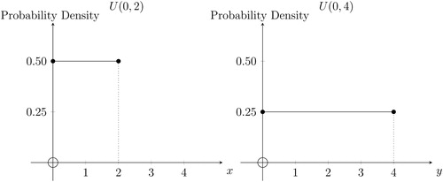
The effect of rescaling can be seen even more simply with a uniform (i.e., rectangular) distribution. Take a dartboard and draw a horizontal ray from the center out to the right. Now throw a dart at the center of a dartboard and measure the angle θ in degrees counterclockwise around to where the dart’s tip pierced the board. Let $X=\theta /180$, then absent any biases, $X\sim U(0,2)$. That is, X is uniformly distributed between 0 and 2 half-revolutions of the dartboard, as shown in the left-hand-side of Figure 9. Now let $Y=\theta /90$, then $Y\sim U(0,4)$. That is, $Y=2·X$ is uniformly distributed between 0 and 4 quarter-revolutions of the dartboard, as shown in the right-hand-side of Figure 9. X and Y measure the same underlying physical phenomenon; it is just that the ruler changes from a count of half-revolutions to a count of quarter-revolutions around the dartboard. The total probability mass is unchanged, but the range of values along the horizontal axis doubles, so there must be half as much probability density over its domain. It is like stretching an elastic fiber to twice its length and watching its linear density (measured in denier) halve, because its mass must be conserved.

Fig. 9 Rescaling preserves Shape II.

NOTE: The left-hand-side density plot shows the uniform density U(0, 2) with pdf $f_X(x)=\frac{1}{2}$ for $0\le x\le 2$ and 0 otherwise. The right-hand-side density plot shows the uniform density U(0, 4) with pdf $f_Y(y)=\frac{1}{4}$ for $0\le y\le 4$ and 0 otherwise. X counts half-revolutions of a dart’s impact point around a dartboard and Y counts quarter-revolutions (see the text).

In all the examples of rescaling given above, both the mean and the standard deviation of the distribution change with the rescaling. Challenge: Can you think of an example of a rescaling where the standard deviation changes, but the mean does not?

9 Conclusion

A survey of 148 final-year students majoring in statistics, physics, and finance revealed a uniformly poor understanding of pdfs. Only 27 out of 148 students (18.2% of our sample) could correctly label the vertical axis as “probability density,” and of these, only five students (3.4% of our sample) could explain their answer. Although incorrect answers to survey questions varied with degree program, there were common misconceptions (e.g., that the vertical access label on a pdf should be “probability,” “count,” or “frequency”). Another commonality was that the proportion of correct answers to our survey questions varied very tightly across degree programs, ranging from only 8.8% of answers correct (in finance undergraduates) to only 12.5% of answers correct (in physics undergraduates).

Thus, our survey revealed poor student knowledge of the basics of pdfs. We argue, however, that such an understanding is part of the foundation of prerequisite knowledge needed to understand the display of data, the building of statistical models, and the conduct of statistical tests. We also argue that the lack of knowledge and misconceptions we found are important multidisciplinary problems.

Garfield and Ahlgren (1988) recommended techniques for overcoming student misconceptions in probability and statistics. In particular, they advise that we recognize and confront common errors of misconception. So, we address these shortfalls in knowledge of pdfs by giving concise explanations and simple examples, some of which appeal to simple physical intuition. We also give intuitive counterexamples to rebut the most common misconceptions revealed by our survey.

The second author has recently used the explanations in this article to teach a class of 100+ final-year undergraduate business students. The students were surprisingly attentive to the material and unusually thankful for it.

Our surprising survey results should grab the attention of every statistics instructor. Our explanations, examples, and counterexamples are useful as assigned reading or as source material for classroom teaching to address the deficiencies across degree programs identified in our survey results.

Acknowledgments

We thank Nicola Beatson, Gurmeet Bhabra, Philip Brydon, David Fletcher, Matthew Schofield, Jeffrey Smith, Jin Zhang, two anonymous referees, and the editors for comments and assistance. Any errors are our own.

Notes

1 We used a small-sample test of differences in proportions assuming independent samples. We simulated 250,000 observations of possible observed proportion pairs for each of 100 different null hypothesis values for the true population proportion. The p-value for a two-sided test was no larger than 3.1% for any of these hypothesized population proportions.

2 If we drop the statistics majors from the sample, $\text{corr}(C,L)=13.3\%$ (t-statistic 1.55) and ${\chi }^2=5.93$ with a p-value of 9.4% (but the expected count is below 5 in two cells).

3 Note that some authors referred to the probability mass function simply as a “probability function” (Spiegel 1975; Evans, Hastings, and Peacock 1994).

4 Note that some authors referred to the cumulative distribution function simply as the “distribution function” (Spiegel 1975; Evans, Hastings, and Peacock 1994). Feller (1968, p. 179) argued that the adjective “cumulative” is redundant.

5 It is possible, however, to create a generalized pdf for discrete or mixed random variables using the Dirac delta function (Chakraborty 2008), but this generalization is above the level of this article.

6 Survey Question 4 asked students to ignore the units. This is because you might argue that height has not changed if units are taken into account. For example, just as with currencies, where 1USD $\approx$ 1.40NZD (i.e., one U.S. dollar approximately equals 1.40 New Zealand dollars at the time of writing), you might argue that $0.20{\text{inch}}^{-1}=0.08{\text{cm}}^{-1}$.

Appendix:

Survey Instrument

A.1 Survey Implementation and Outcomes

Before beginning the survey, the students were told that it contains an example using human height. They were then instructed to read along with the following statement appearing on the reverse of their survey form: “We are assuming that the distribution of human height can be represented and approximated by a theoretical continuous normal distribution. This survey is about that theoretical continuous normal distribution.” (Bold and underlining appearing in the original.) This statement was included to reduce any possible confusion with a discrete pmf.

The reverse of the survey form also included administrative details regarding voluntary participation, ethical approval from our university, and the right to withdraw at any stage. As an incentive, the students were also told that after completion of the survey, a student would be picked randomly to receive a prize but that the student would get the prize only if he/she had made a serious attempt at answering the questions. They were told that a “serious attempt” did not necessarily mean getting the right answers, just that they gave it their best effort.

If you wish to use our survey instrument to test your own students, a softcopy of our survey questions and the verbal instructions we gave our students is available from the authors upon request.

There were two preliminary questions and four subject matter questions, as shown in Appendix A.2. No student withdrew, and of the 148 × 6 = 888 responses called for, only 15 answers were left blank (2, 1, and 12 blanks for Questions 1, 2, and 3, respectively)—a 98.3% response rate. Only one answer out of the 873 answers given was illegible.

Table 3 gives further details on which survey questions our respondents got correct.

A.2 Survey Instrument

Normal Distribution Survey

How many probability or statistics courses are you enrolled in this semester , and how many have you previously completed and passed at university ?

1. Figure A1 shows a theoretical continuous normal distribution representing the height of female students at our university. We have labelled the horizontal axis as “height”. Please write a label for the vertical axis in the box.

   

2. Please define the meaning of the vertical axis label you used above:

   

Fig. A1 Height of female students, measured in centimeters.

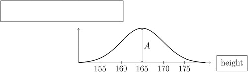
Fig. A2 Height of female students, measured in inches.

1. The horizontal axis in Figure A1 is measured in units of centimeters (cm). What are the units of measurement on the vertical axis (if any)?

   

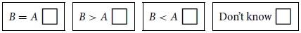
1. Figure A2 shows the same normal distribution of height as shown in Figure A1, but with height measured in inches (where 1 inch = 2.54 cm). How does vertical distance B compare with vertical distance A (ignoring units)? Please tick one box.

References

- Batanero, C., Tauber, L. M., and Sánchez, V. (2004), “Probability Distributions, Assessment and Instructional Software: Lessons Learned From an Evaluation of Curricular Software,” in The Challenge of Developing Statistical Literacy, Reasoning and Thinking, eds. D. Ben-Zvi and J. B. Garfield, Chapter 11, Dordrecht: Springer, pp. 257–276.
- Chakraborty, S. (2008), “Some Applications of Dirac’s Delta Function in Statistics for More Than One Random Variable,” Applications and Applied Mathematics: An International Journal, 3, 42–54.
- Cohen, S., and Chechile, R. A. (1997), “Probability Distributions, Assessment and Instructional Software: Lessons Learned From an Evaluation of Curricular Software,” in The Assessment Challenge in Statistics Education, eds. I. Gal and J. B. Garfield, Chapter 19, Amsterdam, Netherlands: IOS Press (on behalf of the ISI), pp. 253–262.
- Cohen, S., Smith, G., Chechile, R. A., Burns, G., and Tsai, F. (1996), “Identifying Impediments to Learning Probability and Statistics From an Assessment of Instructional Software,” Journal of Educational and Behavioral Statistics (Special Issue: Teaching Statistics), 21, 35–54. DOI: 10.3102/10769986021001035.
- Evans, M., Hastings, N., and Peacock, B. (1994), Statistical Distributions (2nd ed.), New York: Wiley.
- Falk, R., and Konold, C. (1999), “The Psychology of Learning Probability,” in Statistics for the Twenty-First Century, eds. F. S. Gordon, and S. P. Gordon, Washington, DC: Mathematical Association of America, pp. 151–164.
- Feller, W. (1968). An Introduction to Probability Theory and Its Applications (3rd ed., Vol. 1), New York: Wiley.
- Garfield, J., and Ahlgren, A. (1988), “Difficulties in Learning Basic Concepts in Probability and Statistics: Implications for Research,” Mathematics Education, 19, 44–63.
- Judge, G., Hill, R. C., Griffiths, W. E., Lutkepohl, H., and Lee, T.-C. (1988), Introduction to the Theory and Practice of Econometrics (2nd ed.), New York: Wiley.
- Kumar, B. N. P., and Umakanth, R. (2017), “Economic Parameters in Selected Silkworm Races/Breeds of Bombyx Mori l. Using Two Mulberry Varieties,” International Journal of Advanced Scientific Research, 2, 43–46.
- Marshman, E., and Singh, C. (2017), “Investigating and Improving Student Understanding of the Probability Distributions for Measuring Physical Observables in Quantum Mechanics,” European Journal of Physics, 38, 1–24. DOI: 10.1088/1361-6404/aa57d1.
- Ross, S. (1987), Introduction to Probability and Statistics for Engineers and Scientists, New York: Wiley.
- Shukla, S. K. (2017), Fundamentals of Fibre-Reinforced Soil Engineering, Singapore: Springer.
- Spiegel, M. R. (1975), Schaum’s Outline Series: Theory and Problems of Probability and Statistics (16th printing) (2nd ed.), New York: McGraw-Hill.
- Weast, R. C. (1966), Handbook of Chemistry and Physics; A Ready-Reference Book of Chemical and Physical Data (47th ed.), Cleveland, OH: The Chemical Rubber Co.
- Wheat, P., Stead, A. D., and Greene, W. H. (2019), “Robust Stochastic Frontier Analysis: A Student’s t-half Normal Model With Application to Highway Maintenance Costs in England,” Journal of Productivity Analysis, 51, 21–38. DOI: 10.1007/s11123-018-0541-y.