Fitting Percentage of Body Fat to Simple Body Measurements: College Women

Abstract

Percentage of body fat, age, weight, height, and 14 circumference measurements (e.g., waist) are given for 184 women aged 18–25. Body fat, one measure of health, was accurately determined by an underwater weighing technique which requires special equipment and training of the individuals conducting the process. Modeling body fat percentage using multiple regression provides a convenient method of estimating body fat percentage using measures collected using only a measuring tape and a scale. This dataset can be used to show students the utility of multiple regression and to provide practice in model building.

KEYWORDS:

• Best subsets
• Cross-validation
• Forward selection
• Backward elimination
• Least squares
• Multicollinearity
• Multiple regression
• Parsimony

1 Introduction

As is well-documented in the medical literature, obesity is linked with high risk of disease (e.g., Finer 2015). For example, obesity is associated with high risk for both cancer (e.g., Pischon and Nimptsch 2016) and cardiovascular disease (e.g., Elagizi et al. 2018). Also, with respect to the COVID-19 pandemic, the Centers for Disease Control and Prevention (2021a) indicated that obesity increases the risk of both severe illness and hospitalization due to COVID-19 infection. While obesity may be quantified in a variety of ways (e.g., Deurenberg and Yap 1999), one such measure is percent body fat.

In this article, we suggest students predict percent body fat using least squares/multiple regression with the accompanying dataset. Students may be drawn to the body fat data of this article because of the uniform desire for good health. For younger students, the threat of COVID-19 infection will likely be of more immediate concern than that of either cancer or cardiovascular disease. Other articles in this journal discussing fitting a response to multiple predictor variables include Binnie (2004), Carter et al. (2014), Hartenian and Horton (2015), Kuiper (2008), Peterson and Ziegler (2021), and Witt (2013). In addition to containing datasets that are likely to be of interest to a wide range of students, these articles contain anecdotal information on pedagogy useful for improving student performance on least-squares/regression learning outcomes.

Johnson (1996) provided a dataset from Dr. A. Garth Fisher of Brigham Young University giving the percentage of body fat, age, weight, height, and ten circumference measurements (e.g., waist) for 252 men aged 22–81. Percent body fat was accurately determined by an underwater weighing technique which requires special equipment and training of the individuals conducting the process. Building a predictive model for the response variable body fat in terms of the predictor variables age, weight, height, and the circumference measurements then allows men to use this model to estimate their own body fat without undergoing the inconvenient underwater weighing process. Only a tape measure and a scale then need to be used for such prediction.

The dataset associated with Johnson (1996) has had some visibility in the statistical literature. Publications using this data for illustrative purposes and homework include, for example, Faraway (2014), Lock et al. (2017), Matloff (2017), Mills (2005), Mooney and Swift (1999), and Olive (2017). This dataset, in addition to being available at the URL listed in the references (Johnson 1996), may be found within a few R packages including mfp (with data(bodyfat)) and UsingR (with data(fat)).

The dataset accompanying this article is complementary in that, while similar measurements are taken, this time they are from young women. In particular, percentage of body fat (again, through underwater weighing), age, weight, height, and fourteen circumference measurements for 184 female students aged 18–25 from Brigham Young University are given. These data appear in the master’s thesis of Dr. Jason V. Slack (Slack 1997). According to Slack (1997), “a total of 184 females ages 18–25 years were recruited from volunteers attending Brigham Young University. Subjects were notified through physical education activity classes, elementary education teaching classes, and word of mouth.” Dr. Slack (Slack 2021) believed these women to be “mostly Caucasian.” Dr. Fisher, listed above, served as the thesis advisor to Jason Slack. As was the case for the dataset on men, the dataset associated with this article provides a convenient way for young women to predict their percent body fat.

While a handful of different modeling approaches may be made to predicting body fat, including regression trees (Breiman et al. 1984) and neural nets (e.g., Chandra et al. 2016, Garcia and Espinosa 2013), we limit our discussion to prediction using least squares/multiple regression. Principal components analysis might be implemented to address the instability in model coefficients that result as highly correlated measurements are added or removed from a least-squares/regression model (e.g., Manly and Navarro-Alberto 2017). In particular, linear combinations of predictor variables may be used to form “new” predictor variables, but this is not detailed here.

I have used the women’s body fat dataset in just a single offering of the second semester probability and statistics course at my university. The great majority of the roughly thirty students this class had either an industrial engineering or mathematics major. The first semester probability and statistics course in this two-semester sequence includes, among other topics, exposure to descriptive statistics and to hypothesis testing on a single population parameter using p-values. The statistical software package R is also introduced. The second semester course is split fairly evenly between more advanced hypothesis testing (e.g., several population samples) and least-squares/regression. While two semesters of calculus are required for this probability and statistics sequence, calculus should not be viewed as necessary for using the suggested student investigations in this article.

I assigned students to write a polished, word-processed least-squares/regression report (see Appendix A) in which they fit percent body fat for women to the various predictors. They were to show a comprehensive set of approaches to developing such a model, clearly showing their reasoning, verifying any needed assumptions, and commenting on the likely error a female user in the 18-25 age range might encounter. Student learning outcomes were broadly classified as follows:

• Implementing and explaining a variety of model building techniques using either a summary measure (such as adjusted $R^2)$ or p-values, for example,

  • Best subsets

  • Forward selection

  • Backward elimination

• Verifying any needed regression assumptions

  • Including, with discussion, supportive descriptive statistics (e.g., residual plots, normal probability plots)

  • Including, with discussion, hypothesis tests (e.g., formal tests of normality)

• Quantifying the accuracy of their model for young women not used to build their least squares/regression model

  • Using the standard error

  • (Optional) Using cross-validation to get a more honest estimate of the typical error

A rubric for evaluating these least squares/regression projects that addresses the above learning outcomes, as well as quality writing, appears in Appendix B. I did not, by the way, ask students to use any of the predicted body fat models to predict their own body fat. It is virtually certain that some students would be embarrassed to do so.

My basic strategy in discussing model building with least squares/regression, that seemed to work well in previous offerings of this second-semester course, was to first discuss and demonstrate, using other datasets and especially the dataset on men (Johnson 1996), specific smaller topics (e.g., using backward elimination with adjusted R² to fit a response variable) within the broad category of least squares/regression model building. The demonstrations had a dual purpose—an aid to student learning of conceptual topics as well as their developing comfort with the R statistical software. Demonstration R code and relevant data was generally emailed to students prior to class so that students could execute such in class on their own (campus leased and required) computers. Understanding of these specific smaller topics was then assessed with homework exercises (given in Johnson 2020) with feedback prior to further assessment of several of such least squares/regression topics on exams. Graded exams with feedback were returned to students prior to the least squares/regression project for young women being assigned, which was due at the end of the term. The best student projects—and there were a few of these, seamlessly wove together the different aspects of building a model for body fat in a clearly written narrative. At least some of the weaker projects were by students who, as confessed during my office hours, did not allow sufficient time to complete the project.

While I did not conduct a formal survey of reactions to this project, students seemed to enjoy such based on the questions and general interaction I had with a subset of them. Not all students were especially keen on the importance I placed on writing well. (I believe few of the technical classes on our campus contain a significant writing component.) The biggest change I would make in any future least squares/regression project would be to include intermediate assignments to keep students from procrastinating. Such intermediate assignments could include (i) providing an outline (e.g., proposed sections), and (ii) a preliminary draft or drafts. Another obstacle concerned a couple of my students who transferred in credit for the first semester course. They found R to have a rather steep learning curve as their transferred courses did not make use of any statistical software. In the remainder of this article, concepts that tended to be difficult for students are pointed out in the relevant sections.

Numeric computation and graphical displays presented in this article are obtained using version 4.03 of R (R Core Team 2020). Selected R code associated with this article is listed in Appendix C. We often display numeric output to the complete number of decimal digits displayed by R for the sake of reproducibility.

2 Initial Inspection of Data

Percent body fat, Age, Weight (kg), and Height (meters) have already been mentioned as variables. Here is a list of the 14 circumference measurements on the women (all in cm): Ankle, Biceps, Calf, Chest, Elbow, Forearm, Hips, Knee, Neck, DThigh (distal thigh), MThigh (middle thigh), PThigh (proximal thigh), Waist, and Wrist. (Predictor variables are capitalized from here on.) Slack (1997) indicated that these circumference measurements were made “according to the procedures and locations recommended by Lohman, Roche and Martorell” (1988). The remaining variable in the dataset, Body Mass Index (BMI), is calculated as Weight in kilograms divided by squared Height, Height measured in meters. BMI may be viewed, then, as a weight measure with an adjustment for size of body frame. The Centers for Disease Control and Prevention (2021b) suggest “BMI can be used as a screening tool” to help categorize individuals as underweight (BMI < 18.5 kg/m${}^2)$, normal weight (18.5–24.9${\text{kg}/\mathrm{m}}^2)$, overweight (25.0–29.9 ${\text{kg}/\mathrm{m}}^2)$ or obese $(\ge 30{\text{kg}/\mathrm{m}}^2).$ BMI alone has been used to predict body fat (e.g., Mills 2005).

For the various numerical and graphical displays in this article, we retain the units used by Slack (1997). If students are more comfortable dealing with measurements in inches and pounds, then they may perform the appropriate conversions (1 inch $=$ 2.54 cm, 1 kg $\cong 2.205$ lbs) prior to data exploration and analysis.

The bilateral circumferences Ankle, Biceps, Calf, Elbow, Forearm, Knee, DThigh, MThigh, PThigh, and Wrist each refer to measurements on just one side of the body. For researchers who take such measurements, it is standard to always take measurements on a fixed side of the body (Lohman, et al. 1988, chap. 4). Dr. Slack adhered to this practice and believes the measurements were taken on the right side, partly because he currently takes measurements on the right side. He admits, however, that he is not absolutely certain of such as these data were collected many years ago (Slack 2020). The Hips measurement, by the way, is taken across both hips.

Before having students diving into fitting body fat to the other variables, instructors may suggest students consider whether any data values could, in fact, be erroneous. Because of the redundancy of Height, Weight and BMI, the consistency of these three variables may be investigated. Doing so we find that for observation 34 that these three measurements are not consistent. The other observations, up to rounding, do seem to be consistent in these three measurements. Moving away from internal consistency of variables, other errors are apparent, or are at least likely, in the dataset. Boxplots, for example, may be used to identify (likely) errors. Figure 1, for example, shows a boxplot of Age. Slack (1997) indicates that the women in his study ranged in age from 18 through 25 years old. The boxplot shows two outliers: observation 137 concerns the only 25-year-old in the dataset, while observation 120 lists a 1-year-old woman—clearly an error. Table 1 lists other likely recording errors in the dataset; this list is not meant to be exhaustive. See, for example, the article by Holcomb and Spalsbury (2005) for further discussion of data integrity. For the sake of reproducibility, all of the numeric output that follows is done without modifying values in the dataset (without, for example, replacing values as NAs in R).

Fig. 1 Listed Age for the 184 women in Slack (1997).

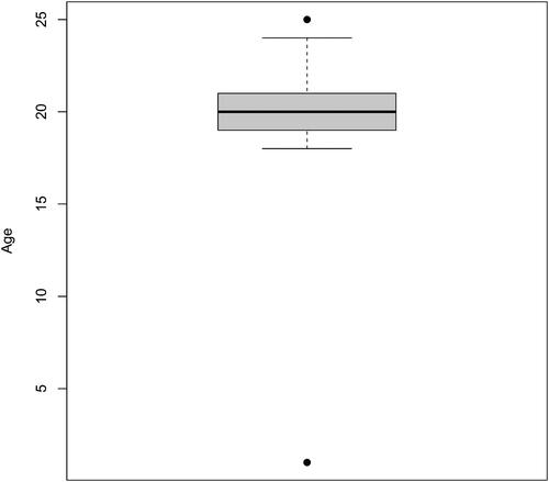
Table 1 Errors/Likely errors in the dataset.

Observation	Error/Likely Error
31	Calf: 66.0 cm
34	Height, Weight, BMI inconsistent
42	Chest: 43.0 cm
120	Age: 1 year
124	Knee: 24.7 cm
135	Chest: 49.5 cm
136	Elbow: 15.5 cm

Helpful Hints: As already suggested, instructors may find it helpful to use the dataset on men (Johnson 1996) to demonstrate analyses they wish their students to be able to perform. Students may then, either individually or in groups, be tasked with similar analyses with the dataset on young women. To make analyses a bit easier, instructors may optionally provide their students with just a subset of the predictor variables. To help prevent copying of work, different subsets of the 184 cases may be used either within a class or across semesters.

3 Simple Numerical and Graphical Analysis

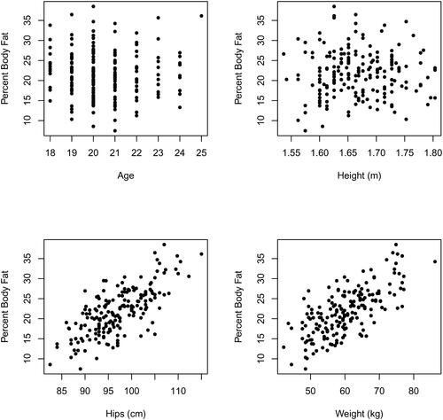
Producing pairwise plots of percent body fat against each of the remaining eighteen predictor variables provides some guidance as to whether particular predictors are useful as well as how predictors may be incorporated into a least squares/regression model. The plots of body fat against Age, Height, Hips, and Weight, for example, are shown in Figure 2. It seems that neither Age nor Height is useful in helping to predict percent body fat while both Hips and Weight should be useful. Examining the other pairwise plots suggests, other than Age and Height, each of the remaining sixteen predictor variables may be useful to at least some degree in predicting body fat. In each of these sixteen scatterplots there is nothing to suggest other than a linear relation between any predictor and body fat exists. So, while pairwise plots only give two-dimensional projections of what is happening in a higher-dimensional space, it is reasonable to try fitting body fat as linear in all the predictor variables excluding Age and Height.

Fig. 2 Fat versus Age, Height, Hips, and Weight. The observation with Age equal to one is omitted from the upper left-hand scatterplot.

To objectively quantify the strength of the linear associations in these pairwise graphical displays Pearson’s correlation coefficient between body fat and the various predictors may be computed. These are shown in Table 2. Since at least some of the various (remaining) sixteen predictor variables are (intuitively) strongly associated, we hope to fit percent body fat by just a subset of these sixteen variables—giving a more parsimonious model. Students may be convinced of the likely redundancy of some of the predictors by examining additional pairwise plots and computing the correlation coefficients between predictors. Figure 3, for example, shows a plot of Weight versus Hips, these variables having a correlation of about 0.885. It seems likely, then, that any final predictive model for body fat would not need to incorporate both Weight and Hips.

Fig. 3 Weight versus Hips.

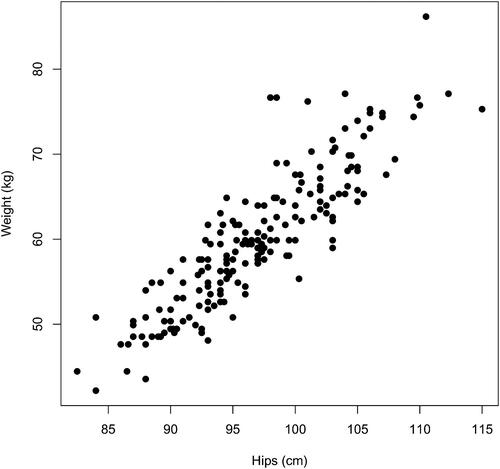
Table 2 Variable correlations (rounded) with Fat.

Variable	Correlation
BMI	0.77
Waist	0.74
PThigh	0.72
Hips	0.71
Weight	0.70
Biceps	0.67
MThigh	0.63
Knee	0.63
Forearm	0.59
Elbow	0.57
DThigh	0.53
Neck	0.50
Wrist	0.50
Chest	0.44
Ankle	0.43
Calf	0.37
Age	−0.06
Height	0.01

4 Least Squares: Best Subsets

In this section we use the best subsets procedure to help build reasonable models for percent body fat. For simplicity, we focus on adjusted R² for measuring model performance. Other measures of performance (e.g., Mallow’s C_p, Akaike’s AIC), of course, may be used instead. Students generally need to be reminded that maximizing adjusted R² is equivalent to minimizing the standard error, or s.e., of regression. In particular,$$\text{adjusted}{R}^2=1-\frac{\mathrm{s}.\mathrm{e}{.}^2}{s_y^2}$$where s_y is the standard deviation of percent body fat. The leaps package in R is convenient for finding the best adjusted R² models for a fixed number of predictor variables. In general, leaps() displays what is referred to as a “best subsets” collection of models. For p total predictor variables (for us, $p=$ 16) and a fixed number of predictor variables, say k, the various $(\begin{array}{c}p\\ k\end{array})$ subsets with k predictors are considered, and the best combination is displayed. To make this a bit more concrete, among the $(\begin{array}{c}16\\ 3\end{array})=560$ subsets of 3 our 16 predictor variables, the subset with BMI, Hips, and Waist produces the best adjusted R². This, along with the best subset for other fixed values of the number of predictors, is displayed in Table 3.

Table 3 Best subsets, according to adjusted $R^2,$ for a fixed number of predictor variables. The highest adjusted $R^2$ occurs when using 9 predictor variables.

	Number of Variables
	1	2	3	4	5	6	7	8	9	10	11	12	13	14	15	16
Adjusted $R^2$(%)	58	61	63	64	65	65	66	66.07	66.19	66.16	66	66	66	66	65	65
Weight						X		X	X	X	X	X	X	X	X	X
BMI	X	X	X	X	X	X	X	X	X	X	X	X	X	X	X	X
Neck											X	X	X	X	X	X
Chest							X	X	X	X	X	X	X	X	X	X
Calf										X	X	X	X	X	X	X
Biceps									X	X	X	X	X	X	X	X
Hips		X	X		X	X	X	X	X	X	X	X	X	X	X	X
Waist			X	X	X	X	X	X	X	X	X	X	X	X	X	X
Forearm													X	X	X	X
PThigh												X		X	X	X
MThigh																X
DThigh															X	X
Wrist				X	X		X	X	X	X	X	X	X	X	X	X
Knee				X	X	X	X	X	X	X	X	X	X	X	X	X
Elbow													X	X	X	X
Ankle						X	X	X	X	X	X	X	X	X	X	X

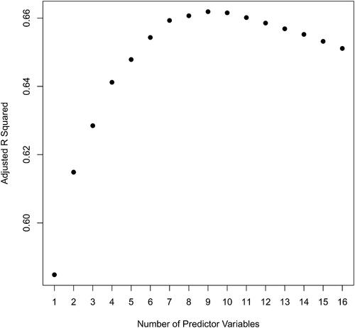
In my experience, students tend to overly focus on single measures of model performance such as adjusted R² to the exclusion of other considerations, notably parsimony. That this was largely not an issue with the least squares/regression assignment may be due to the explicit instruction in this assignment (see Appendix A) to have a balance between accuracy and parsimony. The best adjusted R² model in our case has 9 predictor variables—but this a rather inconvenient number of measurements for a young woman to take to predict her body fat. Notice, from either Table 3 or Figure 4, that the highest values of adjusted R² plateau around about 0.66. It would be much easier for a user to use, say, just three measurements—namely, BMI, Hips, and Waist giving an adjusted R² of about 0.63 which is not too far from the optimum. Using the lm() command in R, we obtain the fitted model$$\begin{array}{c}\text{Predicted Percent Body Fat}=-32.43547+0.80741(\text{BMI})\\ +0.22019(\text{Hips})+0.22170(\text{Waist})\end{array}$$

Fig. 4 Best subsets adjusted $R^2$ versus the number of predictor variables.

The standard error with this model is 3.543%. The residuals range from about –9.35 to 9.43 with a first quartile of about –2.35 and a third quartile of about 2.21.

The above fitted coefficients are not strongly influenced by whether or not the observed values of BMI, Hips, and Waist for any particular woman are included or excluded from the model building process. Cook’s distance, one such measure of influence, is small for each of the 184 observations. While there is lack of agreement as to what constitutes an observation having a large Cook’s distance and high influence, it is not uncommon for practitioners to use a cutoff value of either one or one-half. In the model just fit above, the largest Cook’s distance for the 184 observations was just under 0.068.

While none of the 184 observations apparently have a strong influence on the fitted model coefficients, several of the women have unusual values of BMI, Hips, and Waist compared to the other women. The observations corresponding to these women are referred to as high leverage observations. Observation leverage values lie between 0 and 1 and, if k is the number of predictors (k = 3 in our case) and n is the number of observations (n = 184), the average leverage value is (k + 1)/n. According to one rule of thumb, observations with leverage values greater than three times this average are deemed to have high leverage. With the fitted model on BMI, Hips, and Waist, three of the 184 observations have high leverage (observations 104, 140, and 151 with leverages 0.188, 0.133, and 0.081, respectively). However, none of these high leverage observations are influential. For an observation to be influential in the Cook’s distance sense, the observation must have both high leverage and a residual large in magnitude. The residuals for our three high leverage observations are all “small.” For further details on leverage and influence see, for example, Chatterjee and Hadi (2012).

For instructors using R who wish to discuss leverage and influence, once the output of R’s lm() command is saved (e.g., fit <- lm()), one of the plots produced by a subsequent plot() command (e.g., plot(fit), alternatively par(mfrow = c(2,2)) followed by plot(fit)) will display a scatterplot of (standardized) residuals versus leverage values and flag, by observation number, observations with Cook’s distance larger than one-half and larger than one. Leverage and Cook’s distance are also among the diagnostics output with R’s influence.measures() command.

5 Least Squares: Forward Selection and Backward Elimination Procedures

In this section we briefly examine the forward selection and backward elimination procedures to help build reasonable models for percent body fat. Again, for simplicity, we use adjusted R² for measuring model performance.

Some elementary combinatorics gives a total of $2^p-1=2^{16}-1=65,535$ different models for body fat in terms of various linear combinations of our 16 predictors, containing at least one predictor. I argue in my least squares/regression classes that, because of this exponential explosion in the number of predictors, p, it might be good to have a backup plan to the best subsets procedure, in case our p is moderately large to large.

With forward selection on adjusted R² we start the process by determining the single predictor giving the best adjusted R². This is the same as choosing the predictor with the highest absolute correlation coefficient. According to the correlations listed in Table 2, this is the predictor BMI. Keeping BMI as a predictor, the next forward selection step is adding a second predictor so as to maximize adjusted R². This, after performing the corresponding 15 least-square fits using BMI and one other predictor, is accomplished by adding the predictor Hips. This process continues with, at each step, keeping the j predictors already selected at the previous step and then, after performing the corresponding p – j least-square fits, adding that variable that maximizes adjusted R². Forward selection with our 16 predictors is summarized in Table 4. The best forward selection model is that which has the highest adjusted R². In our case, this involves fitting percent body fat as linear in the nine variables BMI, Hips, Waist, Wrist, Knee, Ankle, Chest, Weight, and Biceps. (The forward selection procedure stops after trying to add Calf to our model as the adjusted R² decreases.) This is also the best subsets model from the previous section, but these two methods do not give the same result in general. Again, for a more parsimonious model, it is desirable to use a smaller number of predictor variables.

Table 4 Forward selection.

Model Predictors	Adjusted $R^2$
BMI	0.5848115
$+$ Hips	0.6148687
$+$ Waist	0.6284737
$+$ Wrist	0.6407330
$+$ Knee	0.6478705
$+$ Ankle	0.6538457
$+$ Chest	0.6593282
$+$ Weight	0.6607029
$+$ Biceps	0.6618973
$+$ Calf	0.6615658
$+$ Neck	0.6601704
$+$ PThigh	0.6585607
$+$ Forearm	0.6568581
$+$ Elbow	0.6552405
$+$ DThigh	0.6532010
$+$ MThigh	0.6511244

Backward elimination starts by including all p predictor variables in the model. At each step one predictor variable is removed. With j predictors in the current model, after performing the corresponding j least-square fits with just one of these predictors dropped, we remove that variable resulting in the highest adjusted R². The process stops if dropping another variable decreases the adjusted R² value. A summary is given in the two left-most columns of Table 5. The reader should verify that using backward elimination gives the same model for body fat as obtained before by both the best subsets and the forward selection process.

Table 5 Backward elimination.

Model predictors	Adjusted $R^2$	Largest Individual $p$-value
All except age, height (16 variables)	0.6511	MThigh: 0.998412
- Mthigh	0.6532	DThigh: 0.937797
- Dthigh	0.6552	PThigh: 0.662902
- PThigh	0.6569	Forearm: 0.65239
- Forearm	0.6585	Elbow: 0.700402
- Elbow	0.6602	Neck: 0.591129
- Neck	0.6616	Calf: 0.363670
- Calf	0.6619	Biceps: 0.205042
- Biceps	0.6607	Weight: 0.19230
- Weight	0.6593	Wrist: 0.05338
- Wrist	0.6540	Chest: 0.04077
- Chest	0.6477	Knee: 0.01902
- Knee	0.6386	Ankle: 0.01491
- Ankle	0.6285	Waist: 0.00634
- Waist	0.6149	Hips: 0.000136
- Hips	0.5848	BMI: < $2\times {10}^{-16}$

In general, in terms of whatever optimization criterion is used (for us adjusted $R^2)$, forward selection and backward elimination may not give models that perform as well as that obtained by the best subsets procedure. By only either adding or subtracting predictor variables (a nested sequence of models), we fail to examine all $2^p-1$ models considered by the best subsets procedure.

We omit discussion of general stepwise procedures that allow for either the addition of a predictor or the removal of a predictor at any given step. Details may be found in any number of regression textbooks (e.g., Draper and Smith 1998).

6 Regression Model Assumptions

Instead of using adjusted R² in the forward selection or backward elimination procedures, one may use p-values of the individual predictor variables (contingent on the other predictor variables in the model). With backward elimination, for example, body fat may be fit to the full model involving all 16 predictors. We then drop the variable with the highest p-value, specifically MThigh, with a p-value of 0.998412. Then body fat is fit to the remaining 15 predictor variables other than MThigh and we again eliminate that variable with the highest p-value. This time it is DThigh with a p-value of 0.937797. This removal process continues (see the left- and right-most columns of Table 5) until all individual coefficient variables have p-values below some threshold. Using 0.05 for this threshold (this is quite common) gives a predictive model for body fat in terms of the predictors Chest, Knee, Ankle, Waist, Hips and BMI (see Table 5). Using 0.01 for this threshold gives the model with only Waist, Hips, and BMI (again, see Table 5). A partial summary of the R output for this three-predictor model appears above in Section 4.

The two sequences of predictor variable deletions—one using adjusted R² and one using individual predictor p-values (nonequivalent measures), need not be the same. In this case they are, and this allows the common sequence to be displayed in Table 5. Typically, the threshold to remove using p-values, as suggested above, is fairly small. The reader should verify from Table 5 that any threshold below 0.205042 will lead to a smaller model using p-values than that optimizing adjusted R².

Forward selection may also be performed using p-values. One problem in doing so using R is that several of our candidate predictors, when used singly, all produce a p-value which is stated as less than $2\times {10}^{-16}$. In this case, the smallest p-value will correspond to the t value which is largest in magnitude. This occurs with BMI. Continuing, we find forward selection here using p-values produces the same sequence as listed in Table 4 using adjusted R². This is not the case in general.

The use of p-values has come under greater scrutiny over the last few years (e.g., Wasserstein and Lazar 2016). Because of this, it is generally considered good practice to supplement their use with other approaches, such as using adjusted R² above. When prediction is the main goal of model fitting, the adjusted R² approach rather than the p-value approach is generally preferred when implementing stepwise procedures. With respect to our dataset, in fact, which contains some highly correlated (multicollinear) predictor variables, some practitioners suggest avoiding stepwise model building with p-values altogether. Multicollinearity leads to greater variability in the estimated regression model coefficients and the resulting weakened statistical power may make it difficult to identify statistically significant predictor variables. See, for example, Chatterjee and Hadi (2012, p. 309), or Faraway (2014, p. 153), for more details.

The trustworthiness of p-values in our forward selection and backward elimination procedures above is contingent upon the multiple regression model assumptions being reasonably satisfied. Below, in brief outline form, is a list of traditional approaches to checking the necessary assumptions:

1. Adequate incorporation of predictor variables

   • Plots of the model residuals against each of the predictor variables (we hope to see residuals randomly scattered about zero for each such plot). These plots supplement plots of the response, body fat, against each of the various predictor variables.

2. Homogeneity of error variance

   • Plot residuals versus the fitted values (we hope to see a uniform band of residuals and not, for instance, different variabilities according to the size of the fitted values). This plot is generally preferred to simply examining plots of the response versus each of the predictors (looking for uniform variability by the size of the predictor).

3. Normality of the errors

   • For a moderate to large number of observations, we may plot a histogram of the residuals (we are looking for a normal shape). For any number of observations, a normal probability plot of the residuals may (also) be examined (we are looking for a linear plot). Formal tests, such as the Shapiro-Wilks test (shapiro.test(), in R) may also be used.

4. Independence of the errors

   • We omit details here other than to say that the violation of this often occurs when dealing with time series data, which we do not have.

Consider the situation, for example, where we have fit percent body fat as linear in the predictors BMI, Hips, Waist, and Ankle. A portion of the R lm() output associated with this fitted model appears in Table 6.

Table 6 Fitting percent body fat to BMI, Hips, Waist, and Ankle.

Coefficient	Estimate	$p$-value
Intercept	−26.1253	$1.61\times {10}^{-6}$
BMI	0.9256	$1.13\times {10}^{-5}$
Hips	0.2840	0.00026
Waist	0.2040	0.01111
Ankle	−0.6481	0.01491

If we are implementing backward elimination using p-values with, say, a threshold of 0.01, then Ankle would be the next predictor to drop provided we can trust these p-values. In Appendix C under “Checking regression assumptions,” R code is provided to perform the suggested checks a, b, c above in this situation (further details are omitted). As these checks can be reasonably shown to be satisfied, we may drop Ankle. This gives the resulting model in the 3 predictors BMI, Hips, and Waist previously discussed toward the end of Section 4.

A not uncommon point of student confusion on the project was the failure to clearly indicate the need to check regression model assumptions at each iteration of stepwise procedures involving p-values.

The fitted model on BMI, Hips, and Waist$$\begin{array}{c}\text{Predicted Percent Body Fat}=-32.43547+0.80741(\text{BMI})\\ +0.22019(\text{Hips})+0.22170(\text{Waist})\end{array}$$may be used to produce point estimates of percent body fat for specified values of BMI, Hips, and Waist, but prediction intervals are also often of interest. For instructors using R, a prediction interval for the percent body fat for a particular woman may be obtained using R’s predict() command. For example, the code sequence

fit < - lm(Fat ∼ BMI + Hips + Waist,

data = women) values < - data.frame(BMI = 22, Waist = 70,

Hips = 97) predict(fit, newdata = values, interval=

’prediction’, level=.95) gives a 95% prediction interval of (15.2%, 29.2%) on percent body fat for a woman with BMI 22 ${\text{kg}/\mathrm{m}}^2,$ Waist 70 cm, and Hips 97 cm. The midpoint of this interval, 22.2%, is the point estimate of percent body fat for a woman having these three measurements. (Bailey 1991 suggests a maximum of 22% body fat for women to have good health.) Changing the argument interval$=$‘prediction’ to interval$=$‘confidence’ within the above predict() command gives a 95% confidence interval of (21.7%, 22.7%) for the mean percent body fat of women with these measurements. The regression model assumptions must hold for these intervals to be trusted. For further details on these intervals see, for example, Faraway (2014).

7 Honest Estimates of Error

Once a fitted model for percent body fat has been chosen, it is appropriate to indicate to model users the typical error to be expected when they use such to predict their own percent body fat. For concreteness, suppose we consider the fitted model involving BMI, Hips, and Waist from Section 4. Here, the listed s.e. of regression is 3.543% body fat. In layperson’s terms, this value is the typical size of a residual.

This s.e. value, however, is likely to be optimistic as this measure is for a model tuned to the given data. Unfortunately, a significant minority of students failed to mention this shortcoming in their least squares/regression project.

This shortcoming of the s.e. may be overcome by performing the following for each j, j running from 1, 2, …, to $n=184$:

• Leaving out observation j, fit body fat to BMI, Hips, and Waist.

• Compute the predicted body fat for the predictor values in observation j using the above fitted model. Also compute the associated residual, call it $e_{(j)}$.

The second step gives a honest error for the jth observation as the jth observation was not used in the building of the associated fitted model in BMI, Hips, and Waist. (The fitted coefficients in the models will generally vary across the values of $j)$. With this leave-out-one cross-validation approach, a more honest estimate of likely user error, is given by$$\text{cross}-\text{validation error}=\sqrt{\frac{1}{\mathrm{n}-(\mathrm{k}+1)}\sum _{\mathrm{j}=1}^{\mathrm{n}}{\mathrm{e}}_{(\mathrm{j})}^2}$$instead of the usual$$\mathrm{s}.\mathrm{e}.\text{of regression}=\sqrt{\frac{1}{\mathrm{n}-(\mathrm{k}+1)}\sum _{\mathrm{j}=1}^{\mathrm{n}}{\mathrm{e}}_{\mathrm{j}}^2}$$ where e_j is the (ordinary) residual corresponding to the jth observation when fitting the full model on all n observations. Here, k is the number of predictor variables (in a model that allows for a nonzero additive constant); k = 3 when using BMI, Hips, and Waist.

While it may appear that this cross-validation process requires n + 1 different least-square fits (see Appendix C for this approach), only one least-squares fit need be made. (The ordinary and cross-validated errors are linked through what is called the ‘hat’ matrix, the details of which may be found in some regression texts. See, for instance, Abraham and Ledolter 2006, pp. 188 and 189.) Omitting further details, the cross-validation error for the model fitting percent body fat in terms of BMI, Hips, and Waist is very nearly 3.62%—a reasonably small estimated typical error.

8 Concluding Remarks

The women’s body fat dataset provided contains the predictor variables Age, Weight, Height, and fourteen circumference measurements along with the response variable (percent body) Fat. These variables were measured on 184 women. This dataset may be used by instructors to illustrate a number of topics in least squares/multiple regression. These include initial numerical and graphical exploration of the data—including data integrity, variable selection/model building, verifying regression assumptions, and providing an honest estimate of the likely error for users. By way of reminder, the data provided are from a sample of convenience of young women who are mostly Caucasian. Fitted models to predict percent body fat should be limited to such users.

To assist instructors who wish to use this dataset in the classroom, a sample assignment and sample grading rubric are included. Relevant R code is also included.

Acknowledgments

Permission to make the data available electronically was kindly granted by Dr. Jason V. Slack, Utah Valley University. I would also like to thank Jason for visiting with me on questions related to the selection of women in the study and how measurements were taken. Thanks are also due to the referees and the editor. Their comments led to an improved presentation.

Supplementary Materials

Dataset (tab delimited text file): BodyFat.txt

Variable Descriptions: BodyFatInfo.txt

Appendix A:

Least Squares/Regression Assignment

Goal: Fit percent body fat to predictor variables for young college women. Details regarding these variables are provided in a separate (Word) file. Likewise, the actual data are provided in a separate (text) file. It is not enough to simply produce a fitted model. You are required to submit a word-processed report explaining your reasoning to justify your final fitted model. Also, your report should comment on the likely accuracy of using your final model for estimating percent body fat for young women not used to fit this model.

You may either work alone or with exactly one partner. (More than one partner is not allowed.) If you have a partner, make sure that both names appear on the report.

Any inanimate resources (notes, textbook, D2L page materials—including class videos, Internet) are allowed. Working with other people (other than your partner, if you have one) is not allowed.

Due Date: The last day of class. Submit either as a Word document or a pdf file (just one file).

Further Details:

• Report Components:

  • Include a Main Report containing reasoning/justification of final model and comments on likely accuracy for young women not used to build this model. A brief introduction and a brief conclusion should be included. Appropriate summary tables and graphics should be included. The main report should not contain any software (e.g., R) specific details (e.g., R commands). Be very selective on including R output. A good rule-of-thumb: If your R output contains information that you do not address in your exposition, then you have included too much R output. Summarizing R output in a different format, however, is most welcome and highly desirable. The main report should not be more than 20 pages (single spaced, 12-point font).

    • Audience: Write to an audience of students who have taken this course before, but need reminding of important details.

    • Be selective on the inclusion of graphics. It is enough, for example, to give illustrative examples of the full analysis you conduct. In particular, I do not need to see every plot of the response (body fat) versus each of the possible predictors in an initial culling of predictors. Likewise, if/when verifying regression model assumptions, I do not need to see every analysis performed. Show me that you understand how to verify these assumptions by illustrative example (e.g., in just one step in the backward and/or forward processes in the transition from one model to the next model).

    • Divide your main report into sections, with headings (Introduction, …, Conclusion).

  • Include, as appropriate, a Reference section (see Technical Matters below).

  • Include an Appendix containing some detail on what R commands were used. A subset of commands used is fine, an exhaustive list of R commands used is not necessary and is not appropriate. You may find it helpful to have headings and, possibly, sub-headings, to organize your listing of R commands. This appendix should not be more than 5 pages (single spaced, 10-point or 12-point font).

  • (Optional) Add, as an additional appendix, the variable descriptions Word file provided (e.g., this would make sense if you would like to refer to such in your main report).

• A Caution:

  • The final model, to some extent, should be a parsimonious model. (Don’t overly obsess on optimizing any one particular measure of model performance.)

• Grading Components:

  • Exposition (clarity, grammar, spelling).

  • Reasoning—giving clear details on your thought process, including justifying any needed assumptions.

  • How comprehensive you are in demonstrating a mastery of the breadth of material presented in class without being verbose.

  • How well you follow the directions in this document.

  • Your attention to appropriate fine detail (e.g., appropriate labels on figures, including units)

• Technical Matters:

  • There is no requirement to use, say, the Equation Editor in Word or LaTeX to render equations—although you are welcome to do so. (There is no penalty for not using such software.) If not using such specialized software, do the best you can in presenting equations/formulas.

  • Reference all sources that you use (e.g., the textbook, any material from the Internet other than that on the D2L course page). For the textbook, if referenced, use:

    • Johnson, Roger (2020), Least Squares & Regression: The Basics Using R, https://leanpub.com/least_squares_regression.

    • You should also cite the R package (execute cite() within R to give an appropriate citation).

  • (Minor Detail) You may find the use of a proportional font such as Courier New in Word to be useful in aligning R output in a more readable way.

Appendix B:

A Grading Rubric

Likert Scale: Excellent (5), Good (3), Average (2), Below Average (1), Poor (0)

In numbered lists (i., ii., …), items incorporated into a report are circled.

1. Model Building:

   • Reasoning 5 3 2 1 0

   • Approaches 5 3 2 1 0

     1. Best Subsets (adjusted $R^2)$

     2. Forward selection (adjusted R², p-values)

     3. Backward elimination (adjusted R², p-values)

     4. General stepwise (adjusted R², p-values) —in text, not discussed in class

     5. AIC, with step command (forward, backward) —in text, not discussed in class

   • Assumption Checking 5 3 2 1 0

     1. Normality (histograms, probability plots, Shapiro-Wilk, 68/95/99.7 rule, invoke CLT variant discussed in text)

     2. Constant variance (response versus predictor, residual plots)

     3. Understood normality checking was needed at each step of forward selection, backward elimination (and general stepwise) when p-values are used

2. Model Accuracy:

   • Comments 5 3 2 1 0

     1. Mentioned that the s.e. is the “typical size of a residual”

     2. Mentioned model is only appropriate for young women, ages 18-25 (or so)

     3. Mentioned s.e. is likely to be overly optimistic (too small)

        Bonus: Cross-validation (mentioned, actually carried out)

3. Use of Summary Tables:

   $\begin{array}{ccccc}5& 3& 2& 1& 0\end{array}$

   1. For stepwise procedures:

      • Forward selection (adjusted R², p-values)

      • Backward elimination (adjusted R², p-values)

      • General stepwise (adjusted R², p-values) —in text, not discussed in class

   2. Best subsets

   3. Miscellaneous:

      • Predictor variable correlations

      • Other (list): _____________________________________

4. Use of Graphics (other than for assumption checking):

   $\begin{array}{ccccc}5& 3& 2& 1& 0\end{array}$

   1. Initial variable culling/correlation with body fat

   2. Other (list): __________________________________________

5. Overall Effort/Comprehensive?

   $\begin{array}{ccccc}5& 3& 2& 1& 0\end{array}$

6. Fine Detail (plot labels, …) and Appearance of Report

   $\begin{array}{ccccc}5& 3& 2& 1& 0\end{array}$

7. Clarity, Grammar, Spelling

   $\begin{array}{ccccc}5& 3& 2& 1& 0\end{array}$

8. Clearly laid out Appendix: R Code

   $\begin{array}{ccccc}5& 3& 2& 1& 0\end{array}$

9. Bonus Items (circle added items):

   • Spotted outliers (age of 1, others)

   • (Optional) Variable descriptions Appendix

   • Used LaTeX, or Equation Editor in Word (no extra credit for these—just an FYI for me)

   • References (Johnson 2020, additional outside references)

Appendix C:

Selected R code

Loading and peeking at the data:

women < - read.table(file.choose(),header = TRUE)

head(women)

Boxplot, Figure 1:

# Display and store boxplot output (pch = 19

gives solid black dots): bp_age < - boxplot(women$Age, ylab="Age",

pch = 19)

# Display outliers:

outliers < - bp_age$out

women[women$Age

Panel of scatterplots, Figure 2:

# To exclude observation 120 with Age = 1: temp < - women[-120,] # Create panel of scatterplots with 2 rows,

2 columns: par(mfrow = c(2,2)) plot(temp$Fat ∼ temp$Age, xlab="Age", ylab="Percent Body Fat") plot(women$Fat ∼ temp$Height, xlab="Height", ylab="Percent Body Fat") plot(women$Fat ∼ temp$Hips, xlab="Hips", ylab="Percent Body Fat") plot(women$Fat ∼ temp$Weight, xlab="Weight", ylab="Percent Body Fat")

Alternative to panel of scatterplots:

pairs(∼ Fat + Age + Height + Hips + Weight, data

=women[-120,], lower.panel = NULL, pch = 20)

Scatterplot, Figure 3:

plot(women$Weight ∼ women$Hips, xlab="Hips (cm)",

ylab="Weight (kg)", pch = 19)

Correlations, Table 2:

cor(women)

Best subsets, Table 3 and Figure 4:

# Install the package leaps using the following

command # after removing the # symbol: # install.packages("leaps") library(leaps) predictors < - with(women, data.frame(Weight,BMI,

Neck,Chest,Calf, Biceps,Hips,Waist,Forearm,PThigh,MThigh,DThigh,

Wrist,Knee,Elbow,Ankle)) labels < - c("Weight","BMI","Neck","Chest",

"Calf","Biceps","Hips", "Waist","Forearm","PThigh","MThigh","DThigh",

Wrist","Knee",

"Elbow","Ankle") # Best subsets, Table 3: leaps(predictors, women$Fat, method="adjr2",

nbest = 1, names = labels) # Store details for Figure 4: output < - leaps(predictors, women$Fat, method=

"adjr2", nbest = 1, names = labels) # Number of predictors is one less than size

which includes beta0 num_pred < - output$size - 1 # Figure 4: plot(output$adjr2 ∼ num_pred, xlab="Number of

Predictor Variables", ylab="Adjusted R Squared", xaxp = c(1,16,15),

pch = 19)

Forward selection, Table 4 (backward elimination, Table 5, is similar):

fit1 < - with(women, lm(Fat ∼ BMI)) summary(fit1) # Two predictor combinations: fit2 < - with(women, lm(Fat ∼ BMI + Weight)) summary(fit2) fit3 < - with(women, lm(Fat ∼ BMI + Neck)) summary(fit3) fit4 < - with(women, lm(Fat ∼ BMI + Chest)) summary(fit4)

.

.

fit16 < - with(women, lm(Fat ∼ BMI + Ankle)) summary(fit16) # Three predictor combinations: fit17 < - with(women, lm(Fat ∼ BMI + Hips + Weight)) summary(fit17) fit18 < - with(women, lm(Fat ∼ BMI + Hips + Neck)) summary(fit18) fit19 < - with(women, lm(Fat ∼ BMI + Hips + Chest)) summary(fit19)

.

.

fit30 < - with(women, lm(Fat ∼ BMI + Hips + Ankle)) summary(fit30)

Checking regression assumptions:

# Table 6 end of section 6,

fitting Fat to BMI,Hips,Waist,Ankle: fit < - with(women, lm(Fat ∼ BMI + Hips + Waist +

Ankle)) summary(fit) # Adequate incorporation of predictor variables: # (Note: The windows() command opens a new

graphics window for the # subsequent scatterplot produced by the plot()

command. It works # for windows computers only.) windows() plot(fit$residuals ∼ women$BMI,

xlab="BMI",ylab="Residuals", pch = 19) windows() plot(fit$residuals ∼ women$Hips, xlab="Hips

(cm)",ylab="Residuals",

pch = 19) windows() plot(fit$residuals ∼ women$Waist, xlab="Waist

(cm)",ylab="Residuals",

pch = 19) windows() plot(fit$residuals ∼ women$Ankle, xlab="Ankle

(cm)",ylab="Residuals",

pch = 19) # Homogeneity of error variance: windows() plot(fit$residuals ∼ fit$fitted, xlab="Fitted

Values", ylab="Residuals", pch = 19) # Normality of errors: windows() hist(fit$residuals, xlab="Residuals", main="") windows() qqnorm(fit$residuals) qqline(fit$residuals) shapiro.test(fit$residuals) # Since assumptions reasonably satisfied, smaller

model appropriate # (Ankle has the highest p-value): smallerfit < - with(women, lm(Fat ∼ BMI + Hips +

Waist)) summary(smallerfit)

Code to compute cross-validation error (Section 7):

# Extract column 5 (BMI), column 11 (Hips),

column 12 (Waist): x < - women[,c(5,11,12)] # Extract column 2 (Fat): y < - women[,2] n < - nrow(women) cv_err < - NULL for (j in 1:n) { # Omit observation j in fit: fit < - lm(y[-j] ∼ x[-j,1] + x[-j,2] + x[-j,3]) b0 < - fit$coefficients[[1]] b1 < - fit$coefficients[[2]] b2 < - fit$coefficients[[3]] b3 < - fit$coefficients[[4]] # Predict fat for observation j: ypred < - b0 + b1*x[j,1] + b2*x[j,2] + b3*x[j,3] # Cross-validated error, observation j: cv_err[j] < - y[j] - ypred} cv_err < - sqrt(sum(cv_err*cv_err)/(n-4)) cv_err

References

- Abraham, B., and Ledolter, J. (2006), Introduction to Regression Modeling, Belmont, CA: Thomson Brooks/Cole.
- Bailey, C. (1991), The New Fit or Fat, Boston, MA: Houghton-Mifflin.
- Binnie, N. (2004), “Using EDA, ANOVA and Regression to Optimise Some Microbiology Data,” Journal of Statistics Education, 12. DOI: https://doi.org/10.1080/10691898.2004.11910738.
- Breiman, L., Friedman, J., Stone, C. J., and Olshen, R. A. (1984), Classification and Regression Trees, Boca Raton, FL: Chapman and Hall/CRC Press.
- Carter, N., Felton, N., and Schwertman, N. (2014), “A Classroom Investigation of the Effect of Population Size and Income on Success in the London 2012 Olympics,” Journal of Statistics Education, 22. DOI: https://doi.org/10.1080/10691898.2014.11889698.
- Centers for Disease Control and Prevention. (2021b), https://www.cdc.gov/obesity/adult/defining.html.
- Centers for Disease Control and Prevention. (2021a), Available at https://www.cdc.gov/obesity/data/obesity-and-covid-19.html.
- Chandra, P., Singh, A. P., and Sehrawat, R. (2016), “Effect of Activation Function Symmetry on Training of SFFANNs with the Backpropagation Algorithm,” 2016 10th International Conference on Intelligent Systems and Control (ISCO), Coimbatore, 2016. DOI: https://doi.org/10.1109/ISCO.2016.7726903.
- Chatterjee, S., and Hadi, A. S. (2012), Regression Analysis by Example (5th ed.), New York: John Wiley & Sons.
- Deurenberg, P., and Yap, M. (1999), “The Assessment of Obesity: Methods for Measuring Body Fat and Global Prevalence of Obesity,” Best Practice & Research Clinical Endocrinology & Metabolism, 13, 1–11.
- Draper, N. R., and Smith, H. (1998), Applied Regression Analysis (3rd ed.), Wiley-Interscience.
- Elagizi, A., Kachur, S., Lavie, C.J., Carbone, S., Pandey, A., Ortega, F. and Milani, R.V. (2018), “An Overview and Update on Obesity and the Obesity Paradox in Cardiovascular Diseases,” Progress in Cardiovascular Diseases, 61, 142–150. DOI: https://doi.org/10.1016/j.pcad.2018.07.003.
- Faraway, J. J. (2014), Linear Models with R (2nd ed.), Boca Raton, FL: CRC Press.
- Finer, N. (2015), “Medical Consequences of Obesity,” Medicine, 43, 88–93. DOI: https://doi.org/10.1016/j.mpmed.2014.11.003.
- Garcia, F., and Espinosa, J. (2013), “Estimation of Body Fat Percentage Using Neural Networks,” Links Magazine, 10.
- Hartenian, E., and Horton, N. (2015), “Rail Trails and Property Values: Is There an Association?,” Journal of Statistics Education, 23. DOI: https://doi.org/10.1080/10691898.2015.11889735.
- Holcomb, J., and Spalsbury, A. (2005), “Teaching Students to Use Summary Statistics and Graphics to Clean and Analyze Data,” Journal of Statistics Education, 13. DOI: https://doi.org/10.1080/10691898.2005.11910567.
- Johnson, R. W. (1996), “Fitting Percentage of Body Fat to Simple Body Measurements,” Journal of Statistics Education, 4, http://jse.amstat.org/v4n1/datasets.johnson.html, dataset: http://jse.amstat.org/datasets/fat.dat.txt, variable descriptions: http://jse.amstat.org/v4n1/datasets.johnson.html, dataset: http://jse.amstat.org/datasets/fat.dat.txt, variable descriptions: http://jse.amstat.org/datasets/fat.txt.
- Johnson, R. W. (2020), Least Squares & Regression: The Basics Using R. Available at https://leanpub.com/least_squares_regression/.
- Kuiper, S. (2008), “Introduction to Multiple Regression: How Much is Your Car Worth?” Journal of Statistics Education, 16. DOI: https://doi.org/10.1080/10691898.2008.11889579.
- Lock, R. H., Lock, P. F., Morgan, K. L., Lock, E. F., and Lock, D. F. (2017), Unlocking the Power of Data (2nd ed.), New York: John Wiley & Sons.
- Lohman, T. G., Roche, A. F., and Martorell, R., Editors (1988), Anthropometric Standardization Reference Manual, Champaign, IL: Human Kinetics Books.
- Manly, B.F.J. and Navarro-Alberto, J.A. (2017), Multivariate Statistical Methods: A Primer (4th ed.), Boca Raton, FL: CRC Press.
- Matloff, N. (2017), Statistical Regression and Classification: From Linear Models to Machine Learning, Boca Raton, FL: CRC Press.
- Mills, T. C. (2005), “Predicting Body Fat using Data on the BMI,” Journal of Statistical Education, 4.
- Mooney, D. D. and Swift, R. J. (1999), A Course in Mathematical Modeling, Mathematical Association of America.
- Olive, D. J. (2017), Linear Regression, Cham, Switzerland: Springer International Publishing.
- Peterson, A., and Ziegler, L. (2021), “Building a Multiple Linear Regression Model with LEGO Brick Data,” Journal of Statistics Education, https://doi.org/https://www.tandfonline.com/doi/full/10.1080/26939169.2021.1946450.
- Pischon T., Nimptsch K. (2016), Obesity and Risk of Cancer: An Introductory Overview (chapter). In Recent Results in Cancer Research (book series), Obesity and Cancer (vol. 208), eds. T. Pischon and K. Nimptsch, Cham, Switzerland: Springer International Publishing.
- R Core Team (2020), R: A Language and Environment for Statistical Computing, R Foundation for Statistical Computing, Vienna, Austria https://www.R-project.org/.
- Slack, Jason V. (1997), “Estimating Body Fat Percentage Using Circumference Measurements and Lifestyle Questionnaire Data: A Multivariate Study of 184 College Aged Females,” M.S. Thesis, Department of Physical Education, Brigham Young University. Available via OregonPDF in Health & Performance, https://www.oregonpdf.org/, Catalog ID: PE 3794.
- Slack, Jason V. (2020, 2021), Personal communications.
- Wasserstein, R. L., and Lazar, N.A. (2016), “The ASA Statement on p-Values: Context, Process, and Purpose,” The American Statistician, 70, 129–133.
- Witt, G. (2013), “Using Data from Climate Science to Teach Introductory Statistics,” Journal of Statistics Education, 21. DOI: https://doi.org/10.1080/10691898.2013.11889667.