A Fresh Shot at Statistics in the Classroom: Three Perspectives Using World Cup Soccer Player Data

Abstract

In this article, we outline several activities revolving around soccer players who participated in the 2018 FIFA World Cup and 2019 FIFA Women’s World Cup. Classroom activities are described from different perspectives, useful for a range of different statistics courses. In a first semester probability theory course, students investigate the counter-intuitive birthday paradox empirically and theoretically. For an introductory data science course, students practice their data wrangling skills using the statistical software R. Additional activities are shared for those instructors interested in emphasizing multivariable thinking in a second semester applied statistical modeling course. The activities shared will provide a range of opportunities for instructors to incorporate the FIFA World Cup data in their own courses. Supplementary files for this article are available online.

KEYWORDS:

• Birthday paradox
• Data science
• Data wrangling
• Intermediate statistics
• Introductory statistics
• Multivariable thinking
• Probability
• Real data application

1 Introduction

Every four years, individuals from around the world tune in to watch soccer’s global event: the FIFA World Cup. Data on the players from the most recent FIFA World Cup tournaments are freely available from two different Wikipedia pages: 2019 FIFA Women’s World Cup squads (2021) (https://en.wikipedia.org/wiki/2019_FIFA_Women’s_World_Cup_squads) and 2018 FIFA World Cup squads (2021) (https://en.wikipedia.org/wiki/2018_FIFA_World_Cup_squads). The data include information on all the players who participated in the 2018 FIFA World Cup and the 2019 FIFA Women’s World Cup including the player’s name, jersey number, team (national and club), the group their national team was in for the first round of the tournament, field position, date of birth, age, the number of caps (games played with the national team), and the number of goals (as of the start of the tournament) for each player. In this article, we introduce different activities utilizing the World Cup data that are useful within a variety of classes including probability, data science, and courses emphasizing multivariable thinking.

When working with the FIFA World Cup and FIFA Women’s World Cup data, students do not need to understand all the particulars of soccer. From our experience, we encourage instructors to outline and have a brief discussion with students regarding the general setup of soccer teams, the FIFA World Cup, and the FIFA Women’s World Cup. This discussion helps students become invested in the activity. For example:

• The FIFA World Cups are international competitive soccer tournaments and are highly followed sporting events attracting viewership from around the world;

• Teams with 23 rostered players per team participate in each tournament;

• Both FIFA World Cups occur every 4 years at different locations (host nation) and the host nation always participates in the tournament;

• 32 teams participated in the 2018 FIFA World Cup (hosted in Russia); and

• 24 teams participated in the 2019 FIFA Women’s World Cup (hosted in France).

For more on the history of the FIFA World Cups, individuals can check out the FIFA World Cup (2020) and FIFA Women’s World Cup (2020) Wikipedia pages here:

• https://en.wikipedia.org/wiki/FIFA_World_Cup

• https://en.wikipedia.org/wiki/FIFA_Women{/%}27s_World_Cup

The activities we share align with the revised Guidelines for Assessment and Instruction in Statistics Education college report (GAISE College Report ASA Revision Committee 2016). In addition, the activities explicitly use technology to support the fact that modern statistical analyses rely on computation (Loy, Kuiper, and Chihara 2019; American Statistical Association 2014; Nolan and Temple Lang 2010).

The guidelines in the revised GAISE 2016 college report include:

1. Teach statistical thinking.

   • Teach statistics as an investigative process of problem-solving and decision making.

   • Give students experience with multivariable thinking.

2. Focus on conceptual understanding.

3. Integrate real data with a context and purpose.

4. Foster active learning.

5. Use technology to explore concepts and analyze data.

6. Use assessments to improve and evaluate student learning.

In the activities that follow we present students with a real-life scenario—FIFA World Cup soccer players (GAISE recommendation #3). We start with an activity for students in an introductory probability course where we outline guiding steps for students to compute probabilities both empirically and theoretically based on the birthday paradox; in this work we focus on using the statistical software R (GAISE recommendation #5). For students in an introductory data science course, we outline two activities. One activity has students practice their data-wrangling skills using R (GAISE recommendations #5). A second activity has students apply their data-summarizing skills to compute probabilities as they are guided through an example of the birthday paradox that focuses on a conceptual understanding of probability (GAISE #2). For two distinct audiences, we have activities that are created around the underlying goal of having students problem-solve their way through a hands-on experience in order to grasp for themselves one of the counterintuitive results of the birthday problem (GAISE recommendations #1 and #2). The activities also are designed for use during a lab setting where students work in cooperative groups to analyze the dataset (GAISE recommendation #4). We end with activities for instructors interested in emphasizing multivariable thinking (GAISE recommendation #5) that provide students more opportunities to engage in an investigative process (GAISE recommendation #1).

2 Overview of the Data

The dataset consists of n = 1288 rows (736 men and 552 women players) and 15 variables. The variables are a mix of identifier, categorical, numerical, and date-time variables. Often students automatically want to assume that all variables whose observations are numbers should be treated as quantitative in all subsequent analyses. These data provide a counterexample to this student misconception. For example, the observations for team ID and jersey number are numerical values; however, these numbers merely represent different identifiers in the dataset. Further, the birth date month and day variables are numerical but represent date-time variables that should not be treated as typical quantitative variables. Instructors may pose to students whether calculations such as taking a median or mean make sense in order to help emphasize this distinction.

In Table 1, we share summary statistics for the quantitative variables age, caps, and goals along with a summary of the field positions of the players (both in total, and separated by men and women players). Although the distributions for age of the players are roughly symmetric, the distributions for the caps and goals are highly right-skewed with outliers; there is also a large spike of zero values for the goals scored. Values for the caps and goals are missing for (the same) 40 women players; and, all play for one of just three different countries (Cameroon, Nigeria, or Thailand).

Table 1 Summary table for the FIFA World Cup soccer player dataset.

	Min	Q1	Med	Q3	Max	Mean	Std Dev
Age (yrs)	16	24	27	30	45	26.8	4.08
Men	19	25	27	30	45	27.4	3.96
Women	16	23	26	29	41	26	4.09
Caps	0	11	26	59	282	39.4	38.2
Men	0	10	25	52	158	35.4	32.0
Women	0	12	29	66.2	282	45.2	45.2
Goals	0	0	1	6	181	5.77	12.3
Men	0	0	1	5	81	4.52	8.81
Women	0	0	1	8	181	7.56	15.8
	GK	DF	FW	MF
Position	168 (0.130)	423 (0.328)	296 (0.230)	401 (0.311)
Men	96 (0.130)	247 (0.336)	158 (0.215)	235 (0.319)
Women	72 (0.130)	176 (0.319)	138 (0.250)	166 (0.301)

Five number summaries, mean, and standard deviation are reported for numerical variables; counts (and relative frequencies) for the categorical variable. Note that for position: GK $=$ Goalkeeper, DF $=$ Defender, FW $=$ Forward, and MF $=$ Midfielder.

The data were collected by copying the tables from the Wikipedia websites (“2018 FIFA World Cup squads” and “2019 FIFA Women’s World Cup squads”) into a spreadsheet (e.g., Excel), followed by some manual data cleaning to remove special characters, accents, etc. from various player’s or club’s names. Merging of the men and women players and cleaning of the date of birth and age variables was performed in R (see Section 4). A final cleaned dataset (soccer.csv), a more detailed description of each variable (Dataset Codebook), and explanations of some of the soccer-specific terms in the dataset along with a brief overview of the game of soccer and the FIFA World Cups (Soccer Overview), are shared as part of the supplementary materials.

3 A Probability Perspective

The birthday problem is a counterintuitive example in probability where one considers how likely, in a group of n people, it is that at least one pair will share a birthday. The birthday problem is a common example used in statistics and probability courses to illustrate an unintuitive probability concept (see, e.g., Bedwell 2002; delMas and Peterson 1998; Falk 2014; Martin 1998; Suess, Trumbo, and Schupp 2005; Whitney 2001). Instructors often introduce this example by establishing a few assumptions: all birthdate days are equally likely for all individuals, there are 365 days in a year and all individuals are independent. Adopting these assumptions, we can compute the probability that at least two individuals share a birthday. Specifically, one result of the birthday problem is that we require only 23 people before we have over a 50% chance that at least two of these people will share the same day of the year as their birthday. This result, or birthday paradox, is often counterintuitive for students. Before any introduction to the birthday paradox, students often guess that a group much larger than 23 is necessary to achieve a 50% chance of at least one pair sharing a birthday.

Our inspiration to use the birthday paradox with professional soccer teams is based on the article, The birthday paradox at the World Cup (Fletcher 2014) which looks at the percent of 23 player teams that have players sharing birthdays during the 2010 Fédération Internationale de Football Association (FIFA) World Cup. In their article, Coincidence: the truth is out there, Matthews and Stones (1998) also use soccer to illustrate the phenomenon of two or more players sharing a birthday; however, their paper discusses the birthday paradox from the perspective of a soccer match that includes 22 total players and one referee. In this article, we follow the setup from Fletcher (2014) and incorporate more recent data. Each team in the 2018 FIFA World Cup and 2019 FIFA Women’s World Cup has a roster of 23 players; therefore, these data provide an advantageous real-world setup for students to explore the birthday paradox; for example, we can rephrase the question to have students explore the percent of teams who have two or more players sharing a birthday. The activity shared below gives an illustration of one of the counterintuitive results; where, in a group of 23 people, the probability of at least one shared birthday is just over 0.5. Using the activities below, students explore the percent of soccer teams (each consisting of 23 rostered players) that have at least two players sharing a birthday (defined as matching day and month, ignoring year).

Probability calculations are often not intuitive for beginning probability students. Many instructors encourage students to use simulations to help check their work on theoretical probability calculations. Although computer simulations are a good tool for connecting theoretical probabilities to empirical probabilities, simulations often remain abstract for students. We present an activity that allows students to calculate empirical probabilities for the birthday problem using real data, compare the results to the probability computed from a larger computer simulation, and finally compare their results to the theoretical probability.

The activity outlined below is introduced during the third week of a 15-week semester in an introductory probability course. At this point in the semester, the class has learned about counting rules, basic set theory, and introductory probability rules. The class meets three times a week for 50 minutes in a classroom and one time a week for 110 minutes in a computer lab. This activity is designed for learning in a computer lab with predefined cooperative groups of 3 or 4 students. For instructors without a computer lab, this activity may be completed in a regular class period where at least one student in a group has access to a computer. Students require no previous experience with R to complete the activity.

Instructors start the activity with the following question: Assume a soccer team has 23 players (with no twins). Assume player birthdays are independent and each day of the year is equally likely: what is the probability at least two of the players share the same day of the year as their birthday? Students take a guess at the answer based solely on their intuition before investigating the empirical and theoretical probabilities. The next sections will outline the three main parts of the activity where students:

1. discover the empirical probability for shared birthdays using real data,

2. compare the real data empirical probability to the empirical probability for shared birthdays using simulation, and

3. compare the two empirical probabilities to the theoretical probability for shared birthdays.

3.1 The Birthday Paradox: Empirical Probability for Shared Birthdays Using Real Data

The first part of the activity allows students to explore real data. During the 2019 FIFA Women’s World Cup there were teams from 24 countries where each squad had exactly 23 players. The birthday information for each member of the squad is presented at the Wikipedia link: https://en.wikipedia.org/wiki/2019_FIFA_Women’s_World_Cup_squads. Alternatively, an instructor can have the class investigate the 2018 FIFA World Cup data which consist of 32 national teams of 23 players each. In what follows, we focus on an illustration using the 2019 FIFA Women’s World Cup teams.

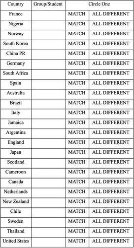
To start off the investigation, the instructor assigns each student a different country (e.g., one of the teams) or assigns small groups of students a few countries each. Each student or group looks up matched birthday information for their assigned countries. To help ensure correct results, it is recommended to assign more than one group or individual to a given country. We have students perform this search during the lab, however, the activity could also be assigned for students to complete before class. After checking their assigned country or countries, students report the countries with no matched birthdays on the squad and countries with at least one matched birthday on the squad at the front of the room. An example chart to keep track of the information is provided in Figure 1. After all groups report their findings, students can answer the following question: What percentage of the 24 teams have at least two players who share a birthday? In this case, 13 of the 24 teams (54.2%) have two players who share a birthday. This can lead to a class or group conversation to determine whether students believe these results are surprising. The discussion provides a nice lead into the simulation part of the activity presented in Section 3.2.

Fig. 1 Example table to use in class to keep track of teams with shared birthdays.

3.2 The Birthday Paradox: Empirical Probability for Shared Birthdays Using Simulation

The following part of the activity involves a computer simulation. A variety of simulations in R have been done using the birthday problem (Suess, Trumbo, and Schupp 2005; Froelich and Larsen 2007; Khitalishvili 2019; Robinson 2020). We walk through an example with our undergraduate students done in the lab. We assume there are 365 days in a year (ignoring February 29th), all birthdays are equally likely, and all the player birthdays are independent. Students are guided through R code to describe the thought process of setting up a simulation. Students are not expected to create the R code themselves and we use R code that does not rely on any outside libraries.

To start, we create the object days in R to represent the possible birthdays during the year. Students use the sample function with replacement to randomly select and display the $n=23$ people’s birthdays from the 365 possible birthdays as represented within the days object. For example,

days <- 1:365 bday_days <- sample(days, 23, replace = TRUE) bday_days

By displaying the days selected in one sample, students can better grasp what the sample function does. One possible sample might look like:

[1] 205 200 353 191 178 141 145 127 138 190 15 45 20 248 40 191 [17] 146 21 274 73 163 81 253

Students are prompted to scan through the sample and determine whether any individuals share a birthday. For example, in this sample students note that two individuals share birthdays on the 191st day of the year. We share with the students one way to automate this process using the unique function:

unique(bday_days)instructing the computer to count automatically how many unique birthdays there are using the length function,

num_unique_bdays <- length(unique(bday_days)) num_unique_bdaysin this case leading to the result:

[1] 22

To estimate the probability empirically that at least two people share a birthday in a sample of size 23, we use R to repeatedly select birthdays randomly with replacement. For each sample, we look at whether two or more people in the sample share a birthday using the function:

bday_fun <- function(size) { days <- 1:365 bday_days <- sample(days, size, replace = TRUE) num_unique_bdays <- length(unique(bday_days)) return(num_unique_bdays) }

We repeat this process using the replicate function in order to compute an empirical probability for any 24 teams. An example of the command in R to repeat this process 24 times is:

nonshared_bday_counts <- replicate(24, bday_fun(23))

To compute the probability that at least two people share a birthday in a sample of 23, we are interested in values of nonshared_bday_counts that are less than 23—as any value smaller than 23 indicates that at least two people shared a birthday in that sample of 23. One way to get this information using R is to add up all the times that nonshared_bday_counts is less than 23. Note that if students have not seen logical values before, instructors are encouraged to show the intermediate step by printing out the vector of TRUE and FALSE (e.g., nonshared_bday_counts < 23) so students can count the number of TRUE values and then find that the total matches the value from the sum (e.g., sum(nonshared_bday_counts < 23)). Students then calculate the empirical probability of at least one shared birthday (e.g., mean(nonshared_bday_counts < 23)).

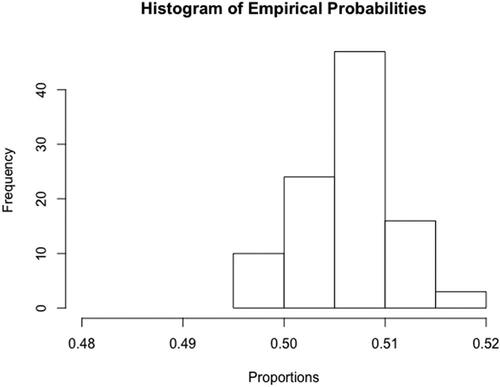
To share their empirical probabilities with the class visually, the instructor has students place post-it notes on the board to create a histogram, or the instructor can collect the values and create a histogram in R. The students will likely see a wide range of values, with a peak close to 0.5. Instructors can discuss with students how empirical probabilities will vary depending on the samples; however, there is some long-run limiting value. To further illustrate the long-run limiting properties, the instructor can propose a hypothetical tournament including 10,000 teams and ask the students how they expect the estimated proportions to change and/or stay the same. Once students have had a chance to brainstorm, instructors run a simulation in R assuming 10,000 teams for each replication (see example code in ProbCourse_Bday.R). Then instructors can plot the estimated sampling distribution for the empirical proportions (an example can be seen in Figure 2).

Fig. 2 Histogram of empirical probabilities for large n.

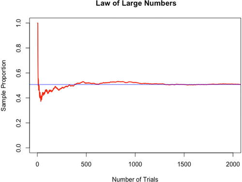
In our experience this is a great place to include a discussion of the law of large numbers (LLN). We emphasize that empirical probabilities based on different samples will differ although they should get closer to the theoretical probability value as the sample size increases. An illustration of the LLN that can be shared with students is in Figure 3. By examining the plot, students can see that as the number of trials increases the empirical probability closes in on a single value (represented by the blue line in Figure 3). Instructors who wish to share the R code with students so that they can recreate the plot themselves, can find this code in the supplementary materials (ProbCourse_Bday.R). This discussion guides students into the final part of the activity where they compute the theoretical probability and recognize its connection with the blue line they observe in Figure 3.

Fig. 3 Illustration of the law of large numbers.

3.3 The Birthday Paradox: Connecting the Empirical Probabilities to the Theoretical Probability for Shared Birthdays

In the last part of the activity the instructor guides students to calculate the theoretical probability for the birthday paradox when we assume 23 individuals. This last part of the activity can be completed during a noncomputer lab class period if needed. As before, we assume there are 365 different possible birthdays (ignoring February 29th) for the 23 individuals, that all birthdays are independent, and all days are equally likely for each player. Using counting techniques previously learned in class, the instructor asks students to determine the number of ways a group of 23 people can have birthdays if we assume random sampling, arriving at the value of 365²³. They then are asked to count the number of ways for 23 people to all have different birthdays. Students recognize that they start with 365 options for the first person, followed by 364 options for the second person and continue until there are 343 options for the 23rd person. The instructor guides students to use properties of complements by asking them to consider what the opposite situation is of “at least one match.” Thus, the instructor guides the students to discover that the theoretical probability is,(1) $$1-\frac{365\times 364\times \cdots \times 343}{{365}^{23}}$$(1)

The computation above represents the probability that at least two individuals share a birthday, leading to a final answer of 0.5073. (For other variations of computing the theoretical probability in R, see, e.g., Johnson 2019 or Murphy 2016.) Comparison of this theoretical probability to both the prior empirical probability calculated based on our sample data (as discussed in Section 3.1) and the simulated empirical probabilities (as discussed in Section 3.2) will help students recognize the relationship between theoretical and empirical probabilities.

3.4 Further Discussions around the Birthday Problem

Before concluding the birthday paradox activity, instructors can guide students through a more in-depth discussion around the assumptions made for the simulation and computation of the theoretical probability. In the activity, students assume that there are 365 days in the year (ignoring February 29th) and that all possible birthdays during the year are equally likely for each player. Students can investigate the equal probability assumption, specific to soccer players, by reading and discussing articles that question the validity of the assumption (see, e.g., Doyle and Bottomley 2018 or Wigmore 2021). Instructors can also share the article by Suess, Trumbo, and Schupp (2005) that discusses using simulation to test the assumption of equally likely birthdays in general. Specifically, they assign weights to the 366 possible birth dates where the weights are consistent with the observed daily birth rates measured in the U.S. (as determined by the National Center for Health Statistics (n.d.) at https://www.cdc.gov/nchs/products/vsus.htm); based on their simulation, no discernable difference is found.

4 A Data Science Perspective

In what follows we outline two activities for introductory data science students: one that focuses on data wrangling and another that has students summarize the cleaned dataset to compute probabilities related to the birthday paradox. The class meets twice a week for 100 minutes, where all students have access to a laptop for every class. The structure and learning goals of the course mirror that of Ismay and Kim (2019) where students first learn about data visualization and data wrangling followed by an introduction to modeling and statistical inference. The activities are done mid-semester, after students have learned the concept of a tidy dataframe (Wickham and Grolemund 2016) and built skills to wrangle and summarize datasets. Specifically, a prerequisite for these activities is that students have some computational skills, specifically with tidyverse in R (Wickham 2017). Both activities we describe are used toward the end of a data wrangling unit (e.g., Ismay and Kim 2019, Ch 1–4) where the students are familiar with the tidyverse verbs such as filter, summarize, group_by, mutate, arrange, join, separate, select, and the pipe operator (Wickham 2017; Wickham and Grolemund 2016; Ismay and Kim 2019). Alternatively, an instructor could weave in the dataset throughout a unit on data wrangling as students learn the different tidyverse verbs. In our experience we found these activities useful if done together to help serve as a bridge between reviewing data wrangling skills to that of introducing concepts of probability (before students begin learning modeling and statistical inference).

The following activities are structured to involve students in the stages of an investigative process (GAISE College Report ASA Revision Committee 2016). To prepare for the class, students read through the information about the FIFA World Cup datasets and become familiar with the variables (see the Dataset Codebook and Soccer Overview files in the supplementary materials). To prompt their curiosity, students consider several discussion questions beforehand; for example:

1. What immediate questions do you have about the data?

2. What questions do you have about the subject matter? What would you like to learn more about? What is unclear?

3. What are some things you would like to learn using these data? Come up with a few questions/hypotheses revolving around the information in these data.

4. In order to clean these data, what do you see as some areas to work on? (You are not expected to clean the data before class, or even know how to do so, as we will be discussing this together in class. At this point we are just brainstorming.)

5. These data have information on the date of birth of the players. Based on your intuition, how many teams do you think will have players that share the same birthday?

We note that question 4 helps to prepare students for our data wrangling activity (see Section 4.1) and question 5 guides students to apply their intuition to a question involving the birthday paradox (see the activity shared in Section 4.2); however, questions 1–3 are useful if further exploration is done with these data (see, e.g., Section 5).

During the 100-minute, lab-based class, students continue their investigative process, being guided through both tidying and summarizing the data, including computing relative frequencies to investigate a counterintuitive result of the birthday paradox. After completing their analyses, students cycle back to their response to question (5) above to see whether the results line up with their intuition. By allowing the students to compute these probabilities themselves, not only do they receive the opportunity to review important wrangling and summarizing tools learned earlier in the semester, but they gain intuition around concepts of probability via the birthday paradox as they are computing and interpreting their own results without simply being told what they should expect.

4.1 Data Wrangling

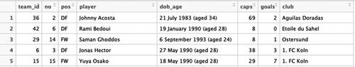
One of the learning objectives for students in our introductory data science course, and often the first key step for any data analysis, is data wrangling (e.g., Ismay and Kim 2019). Before diving into data wrangling with the FIFA World Cup data, students are first asked to make a plan. We pose to them: Our first goal is to create a tidy dataframe. What steps are needed? The question entails that students review and apply the important concept of what constitutes a tidy dataframe (Wickham and Grolemund 2016). The original data for the FIFA World Cup players (playersM.csv) have the date of birth (dob) and age information as a single variable (see Figure 4); so, given our students have recently wrapped up a data wrangling unit, we found they quickly recognize that the dob_age variable needs to be separated. For example, students can separate the parentheses using the regular expression (sep$=$“$\backslash \backslash$(“) or they can separate nine spaces from the right of each observation (sep $=$ – 9) given the consistency of each value in the dob_age variable:

Fig. 4 Example snippet from the original 2018 FIFA World Cup data frame (called playersM in the given R code).

# Option 1 playersM_v1 <- playersM %>% separate(col = dob_age, into = c("dob", "age"), sep= "\\(") # Option 2 playersM_v2 <- playersM %>% separate(col = dob_age, into = c("dob", "age"), sep= -9)

In our experience, students were more comfortable with Option 2, as working with strings and regular expressions (see, e.g., Wickham and Grolemund 2016, Ch. 14) is not a learning outcome of the introductory data science course and thus is not emphasized.

Next, students look closely at the newly separated age variable. In our experience, as this activity was completed at the end of a data wrangling unit, students recognize fairly quickly that R treats the column as a character variable due to the text included in each entry; however, we want age treated as numerical. We ask students to describe the type of variable for age and guide them to functions such as glimpse or View to see how R is actually treating each variable. Once students determine the end goal, the instructor can guide them to consider what tidyverse verb(s) would be useful. One strategy we discuss is to separate the numerical value (what we call age_years below) and remove any unnecessary information (what we call place1 and place2 below). For example, given the consistency of the observations, we can separate each value at the sixth and eighth spaces using sep $=$ c(6, 8); setting convert to TRUE helps to ensure the newly created columns are not all treated as character variables:

# Based on Option 2 above playersM <- playersM_v2%>% separate(col = age, into = c("place1", "age_yrs", "place2"), sep = c(6,8), convert = TRUE) %>% select(-place1, -place2)

After cleaning the age variable, students return to the created dob variable. For the introductory data science course where we implement this activity, students have not yet seen the lubridate library (Spinu et al. 2018; Wickham and Grolemund 2016, Ch. 16). The activity, however, can still provide an example of working with date-time variables and the lubridate library so students are at least aware of its existence. For example, we can format dob correctly into a new variable (DOB) by implementing the mutate function; select(-dob) removes the old, incorrectly formatted, date of birth variable:

men_players2 <- playersM %>% mutate(DOB = dmy(dob)) %>% select(-dob)

After ensuring that the date of birth is treated correctly as a date-time variable, the instructor can walk the students through creating separate columns for the year, day, and month. Separating this information is important for investigating the birthday paradox, since we are ultimately interested in parsing out unique days and months of birthdays for individuals. For example, the instructor can show the students the year, month, and day functions (from the lubridate library) within the mutate function:

men_players <- men_players2%>% mutate( Year = year(DOB), Month = month(DOB), Day = day(DOB) )

The above guided activity is done together as a class with the 2018 FIFA World Cup data. We note that walking through the code in individual steps is not ideal as each intermediate step has the students save the dataset as a separate, new object (which is unnecessarily messy); ideally, we should take full advantage of the pipe operator to create the final dataset (Wickham and Grolemund 2016, Ch. 18). For practice, students complete a similar process and clean the 2019 FIFA Women’s World Cup data (playersF.csv) on their own, or in small groups, while also improving the process by fully implementing the pipe operator. For example, an instructor can give the following prompt: Create a tidy dataframe for the 2019 FIFA Women’s World Cup. You are not allowed to copy and paste. See if you can do it all in one linked statement using the pipe operator. (Still take it step by step!) An example of the code used to clean the playersF.csv dataframe is found as part of the supplementary materials (Data_Wrangling.R).

During the activity, students are curious about what team_ids (see Figure 4) represents. We note that we have these data stored in separate dataframes (teams_men.csv and teams_women.csv). As an additional learning activity, instructors can ask students to merge the men’s and women’s data into a single dataframe (we note this activity assumes a familiarity with the join and bind_rows functions). For example:

mens <- left_join(men_players, teams_men, by = "team_id") %>% mutate(WorldCup = "Mens") womens <- left_join(female_players, teams_women, by = "team_id") %>% mutate(WorldCup = "Womens") soccer <- bind_rows(womens, mens)

The final, cleaned dataset (soccer.csv), original datasets (playersM.csv, playersF.csv, teams_men.csv, and teams_women.csv), and annotated R code for the activity (Data_Wrangling.R) are found as part of the supplementary materials.

4.2 The Birthday Paradox: A Conceptual Understanding of Probability

The birthday paradox does not need to reside solely in a probability course. To guide data science students through the computation needed for an application of the birthday paradox, we start simply. The activity outlined utilizes the final cleaned dataset (soccer.csv), shared as part of the supplementary materials. Students are first directed to look at team #2 for the 2019 FIFA Women’s World Cup and count how many player’s birthdays (ignoring year) match. Although we saw some variety in how students approached this question, most students used functions such as filter, select, and arrange to focus on the one team. For example, the object bdays below is a dataframe of the Month and Days for the birthdays of team #2 players, arranged by month and day:

bdays <- soccer %>% filter(WorldCup == "Women", team_id == 2) %>% select(Day, Month) %>% arrange(Month, Day)

For this one team, students find that two players share a birthday. After successfully finding a match manually, we have the students take this idea and automate the process. We first pose the following, fairly simple, questions for the students (example responses are in parentheses):

• What has to be true for there to be a match? (equivalent values in both columns)

• If there are no matches, how many distinct (i.e., unique) birthdays will there be? (23, since all teams have 23 players rostered)

• If there is at least one match, how many distinct (i.e., unique) birthdays will there be? (fewer than 23)

Once we walk students through the above thought process, they brainstorm how they can automate the process in R, for example: Is there a way we can 1) pull off unique birthdays and then 2) count how many there are? One possible solution uses the distinct and summarize functions:

bdays %>% distinct(Month, Day) %>% summarize(cnt23 = n())

Following the single-team case, students brainstorm how they can extend the idea to apply for all teams. Since we use this activity at the completion of a data wrangling unit, in our experience, students are able to grasp that the group_by function will be useful (other steps may need further guidance, depending on the skill level of the class).

We next walk students through the computations for counting how many teams have matches. For each step, the students brainstorm individually or in small groups before discussing a final strategy as a class.

1. Count how many teams do not have 23 unique player birthdays. That is, mark each team as TRUE or FALSE for whether or not they have 23 unique birthdays. (We remind instructors that this activity occurs after a data wrangling unit, so students are familiar with logical operators (Ismay and Kim 2019, Ch 1).)

2. Compute the proportion of teams with players that share a birthday. That is, we need to know the number of teams, and how many TRUE values there are. (We remind the students that R treats TRUE as 1 and FALSE as 0 when doing computations.)

Following this guided discussion, one possible solution is:

soccer %>% filter(WorldCup == "Women") %>% select(Day, Month, team_id) %>% group_by(team_id) %>% distinct(Month, Day) %>% summarize(cnt = n(), cnt23 = (cnt! = 23)) %>% summarize(num_teams = n(), prop = sum(cnt23)/n())

We note that the final proportion above can be computed as an average using mean(cnt23). However, as our intention is to introduce ideas of probability to our introductory data science students, we find it more helpful to consider the solution in terms of a relative frequency. However, instructors who wish to discuss the computation as an average and its connection to the LLN can reference Section 3.2.

The above guided activity is done for the 2019 FIFA Women’s World Cup data. As practice, students complete a similar process with the 2018 FIFA World Cup data on their own (or in small groups). Example R code (annotated to follow this activity) may be found in the supplementary materials (DataScience_Bday.R). We find 50% of the FIFA World Cup teams and 54.2% of the FIFA Women’s World Cup teams have at least 2 players sharing a birthday which many students find to be surprising.

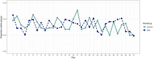
Although these introductory data science students are not expected to compute the theoretical probability, instructors can still share the theoretical result of the birthday paradox to further illustrate that the counterintuitive result students found in their application is not, in fact, unusual. Instructors can further mention that the theoretical probability calculation assumes there are 365 days a year (e.g., ignoring February 29th) and that the birthdate day and month are equally likely for each player. Students can broadly investigate the plausibility of these assumptions being met for the World Cup soccer player data by using their data visualization skills to plot the birthdate days and months for these players (see Figures 5 and 6 and example R code in Exploratory_Analysis.R for an example). Students note that there are some possible dips in the number of players born at the end of the month and at the end of the calendar year. Based on the visualizations, students can discuss whether the number of players needed (for at least a 50% chance that at least two of these people share a birthday) will be larger or smaller accounting for these possible dependencies. To investigate the assumption of 365 days in a year, the instructor can ask the students to investigate whether ignoring February 29th is reasonable for our application. Students discover that one player in the 2019 FIFA Women’s World Cup, forward Stefania Tarenzi who played for Italy, was born on February 29, 1988. Although these discussions are broad in nature, they still align with the learning goals for our audience (introductory data science students): providing a conceptual understanding of probability, including a general appreciation for the implication of possibly violated assumptions. Corresponding R code for the activity may be found in the supplementary materials (DataScience_Bday.R).

Fig. 5 Proportion of players born in each month of the year, computed separately by men and women.

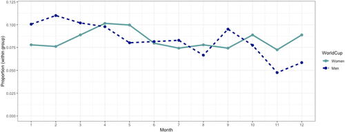
Fig. 6 Proportion of players born on each day of the month, computed separately by men and women.

5 A Multivariable Perspective

Multivariable thinking is desired for any statistics student (GAISE College Report ASA Revision Committee 2016). In this section, we highlight additional examples of how the FIFA World Cup datasets may be used in statistics courses. The examples are not meant to be a comprehensive list, but provide instructors with ideas of additional exploratory questions for students. Corresponding R code for the following examples in Sections 5.1–5.3 is found as part of the supplementary materials (Multivariable_Activities.R).

Before performing any data exploration or analysis, we recommend instructors provide students with a brief overview of the game of soccer and some of the variables they will encounter in the dataset. For example, we have found that many students do not understand what caps are, are unsure what the different field positions represent, and do not understand the distinction between a player’s national team and their club. To aid instructors, we provide a brief summary of these concepts to share with students either as a reading assignment or as a brief discussion in class (see the Dataset Codebook and Soccer Overview files in the supplementary materials).

5.1 Peak Age of Soccer Players

According to the BBC article, When do footballers reach their peak? (Carter 2014), soccer players are expected to peak between 27 and 29 years old. (We will move forward assuming an average of 28 years.) As an exercise, we ask students: Do we have evidence that the 2018 FIFA World Cup and 2019 FIFA Women’s World Cup players support this claim? To answer the question, students perform a two-sided hypothesis test (or construct a confidence interval for a mean). Students find strong evidence ($t=-10.4$, p-value <0.0001) that the 2018 FIFA World Cup and 2019 FIFA Women’s World Cup players are not 28 years, on average. Overall, not only do these data provide instructors with another example of using statistical inference for testing a claim, but the inclusion of a real-world article helps students connect their results to a meaningful context (GAISE recommendation #3). Instructors can further extend the example to encourage multivariable thinking amongst the students (GAISE recommendation #1) by posing questions of whether field position or restricting to men versus women changes the results, for example.

5.2 Number of Goals Scored

One measure of success for a soccer player is the number of goals they score. To investigate differences between the men and women FIFA World Cup players, students can compare the average number of goals scored between the men and the women in the past two FIFA World Cups (note that the measure in the dataset represents the number of goals players scored before the start of the tournament). When students perform a two-sided hypothesis test (or construct a confidence interval for a difference in means), students find strong evidence ($t=-3.94$, p-value < 0.0001) that there is a difference. Considering the greater attention given to the male sport in the professional arena, students may first suspect that the men would have a higher average number of goals scored (as a measure of being more successful players); however, in fact, it is actually the women who scored more goals on average heading into the 2019 FIFA Women’s World Cup. This can lead to discussions about what other factors may go into the women scoring more goals, on average, than the men—such as the number of games played or the competition level of the games (see Longman 2019, as an example of the disparity in teams with the women’s game).

Students also can compare success, as measured by goals scored, across different field positions. For example, consider the ESPN blog post, “What is the most important position? Keeper, defender, midfielder, striker?” (Ames 2016) as a motivating example. Although, as the article suggests, there are many measurements of success in the game, one measurement is the number of goals scored. The main role for a forward player is to score goals; however, part of a midfield player’s role also encompasses being able to score goals for their team. To explore this aspect of the game, students can investigate whether FIFA World Cup caliber players follow these standards by looking at whether forwards do indeed score more, on average, than midfield players. Students can perform a one-sided hypothesis test and find strong evidence (t = 6.6, p-value < 0.0001) that forwards score more than midfielders, on average.

5.3 Influence of Age on Goals Scored

As players become more experienced, we expect them to have more success. Certainly, the older a player is, the more opportunities they have had to score goals. But, the nature of the relationship over time is a matter about which students can conjecture.

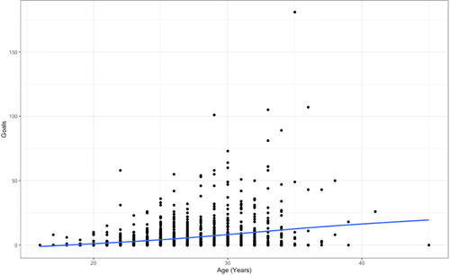
A starting point for exploring this relationship is to visualize the data with a scatterplot and a LOESS curve to determine a reasonable model. As seen in Figure 7, the LOESS curve appears to be fairly linear in nature. (As instructors, we recognize the issue with the increase in variability for older players; however, for the sake of this exercise we are assuming students are unfamiliar or still building familiarity with this concept.) To illustrate the importance of checking both predictive strength and model assumptions, we use this example to discuss R² and residuals. Doing so, students will discover for themselves that what at first might seem to be a reasonable model is not very accurately describing the relationship. For example, the R² value for the linear model tells us only 6.6% of the variability in goals scored is explained by the linear relationship with age. In addition, a residual plot reveals a clear megaphone shape supporting nonconstant variance of the errors and a normal quantile-quantile plot shows a strong skew as evidence against the normality assumption of the errors.

Fig. 7 Scatterplot and LOESS curve for the relationship between age (in years) and goals scored.

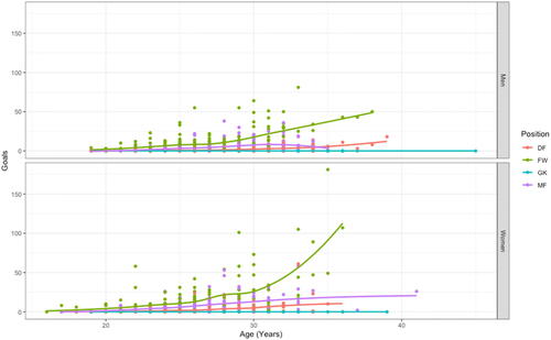
At this point we encourage multivariable thinking by asking students to consider a bigger picture. For example, by separating the data by the four main field positions and the men versus women players (see Figure 8) we see different patterns emerge between the overall goals scored and the age of the players. In particular, there appears to be a multiplicative effect of age with goals scored for the forward (FW) players. One possible hypothesis goes back to who these players are—a nonrandom sample of players selected to play on their nation’s team. The increasing rate of goals scored for forwards as they get older may be related to the selection of these players and the influence goals scored has on their selection as they get older. Alternatively, we may hypothesize the reverse: that forwards who are able to play longer and still be selected for their nation’s team get exponentially better at scoring based on their experience. Looking at midfielders (MF), the relationship between goals and age appears to flatten for older players suggesting that perhaps other criteria are more important for their selection to play on their nation’s team.

Fig. 8 Scatterplot and LOESS curves for the relationship between age (in years) and goals scored separated by position and compared across the 2018 FIFA World Cup and 2019 FIFA Women’s World Cup.

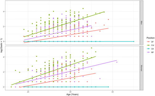
In more advanced applied statistics courses, students can continue their exploration beyond simply visualizing the data and try to improve the simple linear regression model by including more predictors, by transforming the data, and/or by adding quadratic terms. An example is illustrated in Figure 9 where we consider a log transformation (after first adding 1 to each observation) for the response variable of goals scored and consider potential differences across both field positions separately for men and women players.

Fig. 9 Scatterplot of the relationship between age (in years) and goals scored (log(x + 1) transformed) compared across the 2018 FIFA World Cup and 2019 FIFA Women’s World Cup and accounting for differences in field position.

5.4 Additional Investigative Questions to Consider

Regardless of the examples explored, these data provide fodder for interesting discussions on the types of conclusions we can make with a nonrandom sample of data. Discussions can revolve around whether, despite not being random, these data are still representative of some population (and if so, what might that population be).

Other questions for possible consideration include:

• Does the age of a player influence their number of caps?

• Does the average age of a FIFA World Cup player differ between the men and women?

• Investigate the missing values in the dataset. Are they missing at random? If not, what implications does this have?

• Are the proportions of defenders, midfielders, and forwards equally spread out among the players on a team?

• Are the proportions of forwards, midfielders, defenders, and goalkeepers on a team independent of which FIFA World Cup (men’s or women’s)?

• Does the average number of goals (or caps) differ by group (e.g., how teams are grouped for the first stage of the tournament)?

• Some jersey numbers tend to be reserved for certain field positions or players on a team. For example, the jersey number 9 is often worn by the highest scorer on the team (see, e.g., the Wikipedia page, https://en.wikipedia.org/wiki/Squad_number_(association_football)). Is there a relationship between jersey number and the number of goals scored?

6 Conclusion

Whether instructors are teaching a course focused on probability, data science, or multivariable thinking, working with real-world data is vital for students. The examples and activities provided in this work not only revolve around a real-world context for students (the FIFA World Cups) but they further align with the revised GAISE College Report ASA Revision Committee (2016) college report. We hope the activities shared will provide a range of opportunities for instructors to incorporate the FIFA World Cups data in their own courses.

Supplementary Materials

The supplemental materials include all datasets and R code discussed in the article along with the “Soccer Overview” document. The shared datasets, “playersF”, “playersM”, “soccer”, “teams$\_$men”, and “teams$\_$women”, are included as csv files along with their corresponding documentation (“Dataset Codebook”). The R code files, “Data$\_$Wrangling”, “DataScience$\_$Bday”, “Exploratory$\_$Analysis”, “Multivariable$\_$Activities”, “ProbCourse$\_$Bday”, are included with embedded comments to help guide instructors.

References

- American Statistical Association (2014), “Curriculum Guidelines for Undergraduate Statistics Programs in Statistical Science,” http://www.amstat.org/asa/files/pdfs/EDU-guidelines2014-11-15.pdf
- Ames, N. (2016), “What is the Most Important Position? Keeper, Defender, Midfielder, Striker?,” ESPN.com. Available at https://www.espn.com/soccer/blog/espn-fc-united/68/post/2992115/what-is-the-most-important-position-on-a-football-pitch
- Bedwell, M. (2002), “More Happy Returns to the Birthday Problem,” Teaching Statistics, 24, 43–45. DOI: https://doi.org/10.1111/1467-9639.00082.
- Carter, B. (2014), “When Do Footballers Reach Their Peak?,” BBC News. Available at https://www.bbc.com/news/magazine-28254123
- delMas, R. C., and Peterson, W. P. (1998), “Teaching Bits: A Resource for Teachers of Statistics,” Journal of Statistics Education, 6, 3.
- Doyle, J. R., and Bottomley, P. A. (2018), “Relative Age Effect in Elite Soccer: More Early-Born Players, But No Better Valued, and No Paragon Clubs or Countries,” PLoS One, 13, e0192209. DOI: https://doi.org/10.1371/journal.pone.0192209.
- Falk, R. (2014), “A Closer Look at the Notorious Birthday Coincidences,” Teaching Statistics, 36, 41–46. DOI: https://doi.org/10.1111/test.12014.
- FIFA Women’s World Cup Squads (2021), “Wikipedia.” Available at https://en.wikipedia.org/wiki/2019_FIFA_Women’s_World_Cup_squads
- FIFA Women’s World Cup (2020), “Wikipedia,” Available at https://en.wikipedia.org/wiki/FIFA_Women{/%}27s_World_Cup.
- FIFA World Cup Squads (2021), “Wikipedia,” Available at https://en.wikipedia.org/wiki/2018_FIFA_World_Cup_squads
- FIFA World Cup (2020), “Wikipedia,” Available at https://en.wikipedia.org/wiki/FIFA_World_Cup.
- Fletcher, J. (2014), “The Birthday Paradox at the World Cup,” More or Less, BBC Radio 4. Available at https://www.bbc.com/news/magazine-27835311
- Froelich, A., and Larsen, M. D. (2007), Using R in Undergraduate and Graduate Probability and Mathematical Statistics Courses [Conference presentation]. useR!, Ames, IA, August 8–10. Available at https://www.r-project.org/conferences/useR-2007/program/presentations/froelich.pdf
- GAISE College Report ASA Revision Committee (2016), “Guidelines for Assessment and Instruction in Statistics Education College Report.” Available at http://www.amstat.org/education/gaise.
- Ismay, C., and Kim, A. Y. (2019), Statistical Inference via Data Science: A ModernDive into R and the Tidyverse, New York: CRC Press.
- Johnson, I. (2019), “R: Birthday Problem,” R-Bloggers. Available at https://www.r-bloggers.com/r-birthday-problem/
- Khitalishvili, K. (2019), “Birthday Problem Simulation in R,” GitHub Repository. Available at https://github.com/KobaKhit/Bday-Problem-in-R
- Longman, J. (2019), “The Women’s World Cup’s Other Inequality: Rich vs Poor.” The New York Times. Available at https://www.nytimes.com/2019/05/24/sports/womens-world-cup-jamaica.html
- Loy, A., Kuiper, S., and Chihara, L. (2019), “Supporting Data Science in the Statistics Curriculum,” Journal of Statistics Education, 27, 2–11. DOI: https://doi.org/10.1080/10691898.2018.1564638.
- Martin, B. (1998, Sept 9), Fate … or Blind Chance. The Washington Post, H1.
- Matthews, R., and Stones, F. (1998), “Coincidences: The Truth is out There,” Teaching Statistics, 20, 17–19. DOI: https://doi.org/10.1111/j.1467-9639.1998.tb00752.x.
- Murphy, J. (2016), “The Birthday Problem,” RPubs. Available at https://rpubs.com/StatGirl302/TheBirthdayProblem
- National Center for Health Statistics. (n.d.) Vital Statistics of the United States. Centers for Disease Control and Prevention, www.cdc.gov/nchs/products/pubs/pubd/vsus/vsus.htm
- Nolan, D., and Temple Lang, D. (2010), “Computing in the Statistics Curricula,” The American Statistician, 64, 97–107. DOI: https://doi.org/10.1198/tast.2010.09132.
- Robinson, D. (2020), “The Birthday Paradox Puzzle: Tidy Simulation in R,” R-Bloggers. Available at https://www.r-bloggers.com/the-birthday-paradox-puzzle-tidy-simulation-in-r/
- Spinu, V., Grolemund, G., Wickham, H., Lyttle, I., Constigan, I., Law, J., Mitarotonda, D., Larmarange, J., Boiser, J., and Lee, C. H. (2018), “lubridate: Make Dealing with Dates a Little Easier.” Available at https://cran.r-project.org/package=lubridate
- Squad Number (association football) (2020), “Wikipedia.” Available at https://en.wikipedia.org/wiki/Squad_number_(association_football).
- Suess, E., Trumbo, B., and Schupp, C. (2005), “SIMULATION: Computing the Probabilities of Matching Birthdays,” STAT, The Magazine for Students of Statistics, 43, 3–7.
- Whitney, M. C. (2001), “Exploring the Birthday Paradox Using a Monte Carlo Simulation and Graphing Calculators,” The Mathematics Teacher, 94, 258–262. DOI: https://doi.org/10.5951/MT.94.4.0258.
- Wickham, H. (2017), tidyverse: Easily Install and load the tidyverse.
- Wickham, H., and Grolemund, G. (2016), R for Data Science: Import, Tidy, Transform, Visualize, and Model Data. Boston: O’Reilly Media, Inc.
- Wigmore, T. (2021), “Why Athletes’ Birthdays Affect Who Goes Pro—And Who Becomes A Star.” FiveThirtyEight. Available at https://fivethirtyeight.com/features/why-athletes-birthdays-affect-who-goes-pro-and-who-becomes-a-star